The Effect of Systematic Default Risk on Credit Risk Premiums

Abstract

This study examines whether systematic default risks affect a cross section of credit risk premiums. Using a structural framework, I derive a theoretical cross-sectional relationship, develop a testable hypothesis, and provide a method to estimate the systematic default risk. The empirical results of US corporate credit default swap data are consistent with my hypothesis. The findings show that, while credit market factors have positive effects on a cross section of credit risk premiums, stock market factors have a negative impact. Regression analyses reveal that the market’s average default probability and the value factor have a significant effect on the credit risk premium. In addition, credit market factors are more influential than equity market factors as systematic default risk factors. The results suggest that systematic and idiosyncratic default risks are priced differently in a cross section of credit risk premiums.

1. Introduction

Even though credit risk events, such as debt restructuring, bankruptcy, and payment default, are firm specific, they have the potential to affect not only the sustainability of the firm (in terms of assured incomes) but also that of the economy overall. Hence, managing the risks arising from such events is important. It might be questionable how corporate default events harm the wider financial system; however, there are prominent examples of this effect: for instance, subprime mortgage loan defaults in the US in 2007 triggered bankruptcies in the financial sector, such as the Lehman Brothers bankruptcy and the American International Group (AIG) bailout, and eventually led to the global financial crisis (often referred to as a credit crisis). Since the crisis, studies have reported that the timing of loan defaults is more significantly clustered than market participants expected. Therefore, credit risk is not just an issue for individual firms, but for the overall economy as well.

The credit default swap (CDS) was invented to insure the loss arising from corporate bond defaults. A CDS provides buyers with protection against loss and transfers the risk to those who are more willing to endure the risk and seek a lower amount of cash flow. The growth of the CDS market is surprising. According to the Bank for International Settlements, the notional amount outstanding under single-name CDSs had skyrocketed to $33,484 billion in 2007. This figure has since dropped, amounting to $395 billion as of 2018; however, the CDS market continues to be large.

The popularity of the financial instrument is owing to the fact that both academics and practitioners believe that CDSs can provide many benefits. For example, CDSs can detach credit risk from corporate bonds, which allows firms to borrow capital more easily. CDS trading provides information on how the market evaluates the current credit condition of a reference entity. Therefore, such liquidity makes markets more efficient in terms of information. However, there has also been criticism that the abuse of CDSs amplified the occurrence of spiral defaults during the financial crisis (this controversy was well-documented by Stulz [1]). Thus, despite its popularity, we lack a comprehensive understanding of CDSs.

A better understanding of CDS could have implications for sustainability related to credit risk. As witnessed during the 2008–2010 global crisis, defaults are correlated, clustered, and even contagious [2,3,4,5,6]. Thus, there appear to be certain factors that affect almost all firms simultaneously. In this study, I define this as the “systematic default risk.” Economically, systematic default risk can be viewed as the risk that affects the default probabilities of all firms in an economy. My interest lies in how the systematic default risk is priced in CDS spreads in order to investigate the role of systematic default risk.

Hence, it is important to understand the nature of the systematic default risk and the CDS market; however, little is known about the risk premiums for bearing systematic default risks, either theoretically or empirically. This is partly because most previous studies have typically focused on the factors determining CDS spread levels, changes in these levels, and on the pricing of CDS spreads. For example, Merton [7] first constructed a framework to analyze the value of corporate bond spreads and suggested that leverage ratio, asset volatility, and risk-free rate are the most important determinants. Many studies [8,9,10] found empirical evidence to partly support this theory.

Unlike these studies on CDS pricing, I analyze the risk premium component in a CDS spread. CDS spreads are determined not only by expected loss based on the expected default probability but also by the future movement of default probability [11,12,13]. Therefore, the total spread is a sum of these two components. The CDS spread component that is determined by the latter is called a credit risk premium (CRP). For example, given total uncertainty regarding the future dynamics of default probability, if a firm’s default probability is likely to be higher when the entire market default probability is high, investors demand a higher risk premium to offset this risk. Therefore, analyses on total risk cannot fully explain the economic nature of the CRP component. Therefore, understanding how CRPs are associated with systematic default risk is as important as understanding the pricing of total CDS spreads. As such, I attempt to address two questions. (1) What is the potential systematic default risk factor affecting almost all firms’ default risk? (2) Do investors price the systematic default risk and idiosyncratic risk differently in CRPs? Answering these questions could yield valuable insights into the role of systematic default risk.

Within Merton’s framework [7], which provides a theoretical price of CDSs, I derive a theoretical relationship between CRPs and systematic default risks. I accordingly suggest the following hypothesis: “If the price of a systematic asset risk is positive (negative), credit risk premiums are higher (lower) for firms with higher systematic default risk after controlling for the total default risk.” In order to test this hypothesis, I suggest a method to decompose total risk into systematic and idiosyncratic parts and measure the systematic default risk amount using the CDS spread, stock price, and accounting data. The empirical evidence supports my hypothesis. I also find that overall market creditworthiness is the most important factor determining systematic default risk.

An economic implication of my model is that, even though the asset values of two firms are equally volatile, if one firm’s asset value (or default probability) is more sensitive to the systematic default risk that affects the entire economy, then investors will request a higher premium for taking such credit risk, or CRP. In other words, the more likely that a firm’s default probability co-moves with the overall market default probability, the more premium investors will demand for taking such risk.

The results of this study contribute to existing literature on the subject in that I provide a new approach to and evidence on two famous puzzles in finance. Many studies have tried to link equity and credit markets based on Merton’s framework [7], in which corporate bonds can be viewed as a put option written on the firm’s asset value. At the same time, equity can also be viewed as a call option written on the same asset value. Owing to this put-call parity, the two securities’ values are associated with each other. However, empirical studies based on this theory have found two perplexing results. First, previous studies have examined whether credit risk can explain equity returns, without much success. This is called the distress risk puzzle [14,15]. While the theory predicts that stocks with higher credit risk would earn a higher return in the future, the empirical results were opposite to the prediction. Second, using Merton’s framework, researchers examined if credit spreads (corporate bond yield in excess of the risk-free rate) can be explained by equity market information. However, almost all studies have failed to calibrate the empirical observations of credit spreads with equity market data. This is called the credit spread puzzle [16]. As such, while the option pricing theory is simple and clear, the empirical results have been somewhat ambiguous.

My hypothesis is different from the previous studies in that I examine credit risk premiums rather than credit spreads and investigate the relation between credit risk premiums and systematic risk factors such as equity market risk and credit market risk. By doing so, this study provides some evidence that supports Merton’s theory. The theoretical contribution of this study lies in the fact that it provides a CDS pricing model within Merton’s framework and derives a relationship between credit risk premiums and systematic default risk. In terms of methodological contribution, I suggest a way of estimating systematic default risk using CDS spread data, which can also be applied to future work. This study also contributes empirically to the growing literature on credit risk premiums, a topic that has been studied relatively less compared to equity risk premiums.

2. Theoretical Background

This section describes the fundamental framework where I will develop the hypothesis to test in this study. Reviewing some papers which offer a theoretical background, I introduce the models that I will employ in the hypothesis development section.

2.1. The Merton Model

Merton [7] and Black and Scholes [17] showed that a firm’s equity can be seen as a call option with an underlying asset of the firm’s assets $V$, a strike price of default point $D$, and a maturity of T. The hypothesis of my study is developed in the Merton framework, and I briefly introduce his model in this section.

The Merton model assumes that a firm’s asset value follows a long normal process,

$$\frac{dV}{V}=\mu dt+\sigma dZ,$$

(1)

where $V$ is the value of the assets that firm is holding, $\mu$ is a constant expected growth rate of the asset value, $\sigma$ is asset volatility, and $Z$ is the standard Wiener process. Thus, the asset return follows a geometric Brownian motion process. Another assumption is about default timing. At time T, a firm defaults when its asset value drops below some default point $D$ at maturity $T$, i.e., $V\left(T\right)<D$. If the firm defaults, nothing is left for shareholders. Otherwise, shareholders’ value is the residual asset $V\left(T\right)-D$. Then, the shareholders’ value at time T is $\max \left(V\left(T\right)-D,0\right)$. From the bond holders’ perspective, the corporate bond values at T is given by $\min \left(V\left(T\right),D\right)=D-\max \left(D-V\left(T\right),0\right)$. Note that the Merton model does not allow for any default event until the maturity T; defaults can occur at time T only. This assumption makes the story simple.

With these assumptions, the risk-neutral pricing approach provides the current value of equity of the firm.

$$Equity=E^Q\left[e^{-rT}\max \left(V\left(T\right)-D,0\right)\right]=BSCALL\left(V,D,T\right)$$

(2)

and the current value of a corporate bond of the firm.

$$Bond=E^Q\left[e^{-rT}(D-\max \left(D-V\left(T\right),0\right))\right]=D{e}^{-rT}-BSPUT\left(V,D,T\right)$$

(3)

where $E^Q\left[·\right]$ denotes the expectation under a risk-neutral probability, and $BSCALL\left(V,D,T\right)$ and $BSPUT\left(V,D,T\right)$ are the Black-Scholes call and put option pricing formula [7,17], given underlying asset value $V$, strike price $D$, and maturity $T$.

Using $V=Bond+Equity$, we can see that there exists a relationship between put and call option prices, which is called put-call parity. In the Merton framework, the put-call parity can be expressed as

$$Put-Call+V=D{e}^{-rT}$$

(4)

where $r$ is the risk-free rate, $D$ is a default point, and $V$ is a firm’s asset value at the current time. Call and Put denote current prices of call and put options written on the same underlying asset V with a maturity of T. The put-call parity tells us that put option value, call option value, and underlying asset value have a constant relation; note that in the Merton framework, $D$ is a constant value. This means that if the asset value increases, the put value decreases, the call value increases, and subsequently, the spread between put and call decreases as much as the asset value increases. In the view of the Merton model, CDS is a put option on the same firm asset, as will be discussed in the following section. Therefore, it is straight forward that equity prices move in the opposite direction of change in CDS spreads.

2.2. CDS Pricing

A credit default swap (CDS) can be seen as a put option written on the reference entity’s assets [13]. A credit default swap contract is a swap between a regular insurance premium and compensation of loss given default (LGD). For example, a CDS seller receives a premium, which is called a CDS spread, on an annual basis. Instead, the seller promises to pay the buyer the amount as much as the loss of default on debt. Since this contract is a swap, the initial cost is zero.

With this notion, a CDS can be expressed as a combination of long on an annuity and short on a put option [13,18]. From the seller’s perspective, (i) the seller will have been paid off an annuity stream of a CDS spread $s$ until time $T$ and (ii) the seller ought to pay $D-V\left(T\right)$ if $V\left(T\right)<D$. The second cash flow is the same with the cash flow of put option seller that is written on the firm’s asset value with a strike price of $D$ and an expiration of $T$. Since the initial cost of this swap contract is zero, the present values of the two cash flows should be the same, i.e.,

$$s\times PVIFA=BSPUT\left(V,D,T\right),$$

(5)

where $PVIFA$ is the present value of $1 annuity for $T$ years and $BSPUT\left(V,D,T\right)$ is the Black-Scholes put option pricing formula [7,17] with underlying asset value $V$, strike price $D$, and maturity $T$. Without loss of generality, I assume that $PVIFA=1.$ Inserting the put option pricing formula, the theoretical CDS spread can be expressed as

$$s_t=BSPUT\left(V,D,T\right)=D{e}^{-rT}N\left(-d_2\right)-V_{t}N\left(-d_1\right)$$

(6)

where $r$ is the risk-free rate, $N\left(·\right)$ is a standard normal distribution function, and $d_{1,2}=\frac{\ln \left(\frac{V}{D}\right)+\left(r\pm \frac{1}{2}\left({\alpha }^2+{\gamma }^2\right)\right)T}{\sqrt{T\left({\alpha }^2+{\gamma }^2\right)}}$. Thus, Equation (5) tells us that a CDS spread can be seen a put option written on the reference entity’s asset value.

2.3. Credit Risk Premiums

Pan and Singleton [19] and Berndt et al. [11] defined a credit risk premium implicit in a CDS spread in a similar way. Their logic is based on the fact that a CDS spread is determined by an expected part due to default probability and a risk premium. Thus, the risk premium can be obtained by the difference between the observed CDS spread and the expected component of CDS. Especially, Pan and Singleton [19] defined the expected component of CDS spread by a pseudo-CDS spread, as denoted by $s^P$. Then, they define a credit risk premium CRP as

$$CRP=s-s^P,$$

(7)

where $s$ is an observed CDS spread. Pan and Singleton [19] and Berndt et al. [11] employed different methods in order to estimate pseudo-CDS spread $s^P$. Berndt et al. [11] used a structural approach based on the Merton framework. Thus, using equity and accounting information, they estimated expected default probability. On the other hand, Pan and Singleton [19] suggested a new approach based on a reduce-form model. I use both approaches and the details about the estimation procedure will be given in the methodology section.

In the Merton framework, the pseudo-CDS can be defined as

$$s^P=E^P\left[e^{-rT}\max \left(D-V\left(T\right),0\right)\right],$$

(8)

where $E^P\left[·\right]$ is an expectation under the physical measure of probability. Therefore, CRP is the difference between the Q- and P-expectation of the future payoff.

3. Hypothesis Development

There are $N$ firms in the economy and their asset values (or firm values) $V$ stochastically evolve as

$$\frac{d{V}_i}{V_i}={\mu }_{i}dt+{\beta }_{i}dF+{\gamma }_{i}d{W}_i,$$

(9)

where $V_i$ is the value of the assets of firm i, ${\mu }_i$ is the constant expected growth rate of the asset value, $F$ is a systematic risk factor in the economy that affects all firms’ asset values at the same time, and $W_i$ is the idiosyncratic risk of firm $i$. The parameters ${\beta }_i$ and ${\gamma }_i$ determine the sensitivities of the asset value to the systematic risk factor and idiosyncratic risk factor, respectively. We assume that $F$ and $W_i$ are independent standard Brownian motions. This setting is based on the Merton model [7], but the difference is that I decompose the systematic and idiosyncratic parts in order to show their respective roles clearly. Thus, the asset value of this model is also a geometric Brownian motion process.

Next, I define a default event as follows. A firm defaults when its asset value drops below some default point $D_{\mathrm{i}}$ at maturity $T$, that is, $V_i\left(T\right)<D_i$. Ideally, the default point will be the value of a debt obligation with a maturity of $T$ if there is only a single debt obligation. In the empirical analysis, I use the value of current debt plus a half of long-term debt as a default point, as is common throughout the literature [8,9,16,20,21,22]. For simplicity, I also assume that the default event can occur only at maturity time $T$. From now on, for the purpose of simplicity, I omit the subscript $i$ whenever its meaning is clear in the context.

With this model setting, I develop a testable hypothesis regarding credit risk premiums. Let $\lambda$ be the market price of systematic risk (I keep this identical for all firms in the economy through the principle of no arbitrage). Therefore, the expected rate of change in asset value in excess of the risk-free rate should be the systematic risk amount times the unit price of the systematic risk—that is, ${\mu }_i-r={\beta }_i\lambda$. In other words, as the market price of risk is constant for all firms in the economy, the ratio $\lambda =\left({\mu }_i-r\right)/{\beta }_i$ is constant for any i.

Now I define systematic default risk. A default event occurs if the asset value at time T is less than a default point, or $V_T<D$. Therefore, default probability is determined by the current asset value, and fluctuates depending on the future fluctuation of asset value. In general, credit risk is defined by the degree of default probability fluctuation, and a CRP is compensation for taking such risk. Going one step further, I define systematic default risk as the default probability fluctuation owing to a change in the asset value induced by a systematic risk factor $F$, as shown in Equation (9). Differently put, we can decompose the source of the asset value change into two components, systematic risk $F$ and idiosyncratic risk $W_i$. As there are two driving forces for asset value dynamics, some change in asset value is induced by the systematic risk evolution, while the remaining change is caused by the idiosyncratic risk. Subsequently, the systematic default risk is determined by the asset value change induced by the systematic risk. Similarly, the idiosyncratic default risk is determined by the asset value change induced by the idiosyncratic risk. These respective responses are measured by $\beta$ and $\gamma$, respectively.

Economically, systematic default risk can be viewed as the risk that affects the default probabilities of all firms in an economy. My interest lies in whether each component of default risk is differently priced in CDS spreads and in investigating the role of systematic default risk. To see this role clearly, let $p$ be the systematic default risk proportion. Then, it can be defined by $p\equiv {\beta }_i/\sqrt{{\beta }_i^2+{\gamma }_i^2}$. To analyze the effect of systematic default risk on CRPs, we compute a partial derivative with respect to $p$.

As shown in Equations (5), (7), and (8) in Section 2, CRP is the difference between put option values priced under the Q- and P-measures. Then, CRP can be expressed as

$$CRP=D{e}^{-rT}\left[N\left(-d_2\right)-N\left(-d_2^{*}\right)\right]-V_t\left[N\left(-d_1\right)-N\left(-d_1^{*}\right)\right]$$

(10)

where $d_{1,2}^{*}=\frac{\ln \left(\frac{V}{D}\right)+\left(r+\beta \lambda \pm \frac{1}{2}\left({\alpha }^2+{\gamma }^2\right)\right)T}{\sqrt{T\left({\alpha }^2+{\gamma }^2\right)}}$. Using the Black-Scholes put option delta formula, I derive the following:

$$\frac{\partial \mathrm{CRP}}{\partial p}=\lambda \sqrt{T}\left(\left[D{e}^{-rT}\varphi \left(d_2+p\lambda \sqrt{T}\right)-V\varphi \left(d_1+p\lambda \sqrt{T}\right)\right]\right)$$

(11)

where $\varphi \left(·\right)$ is the standard normal density function and the other notations are defined as before. For simplicity, I drop PVIFA as it is just a constant. It is difficult to analytically prove the sign of the derivative value. Instead, I simulate $\frac{\partial \mathrm{CRP}}{\partial p}$ to provide some reasonable values of inputs and parameters.

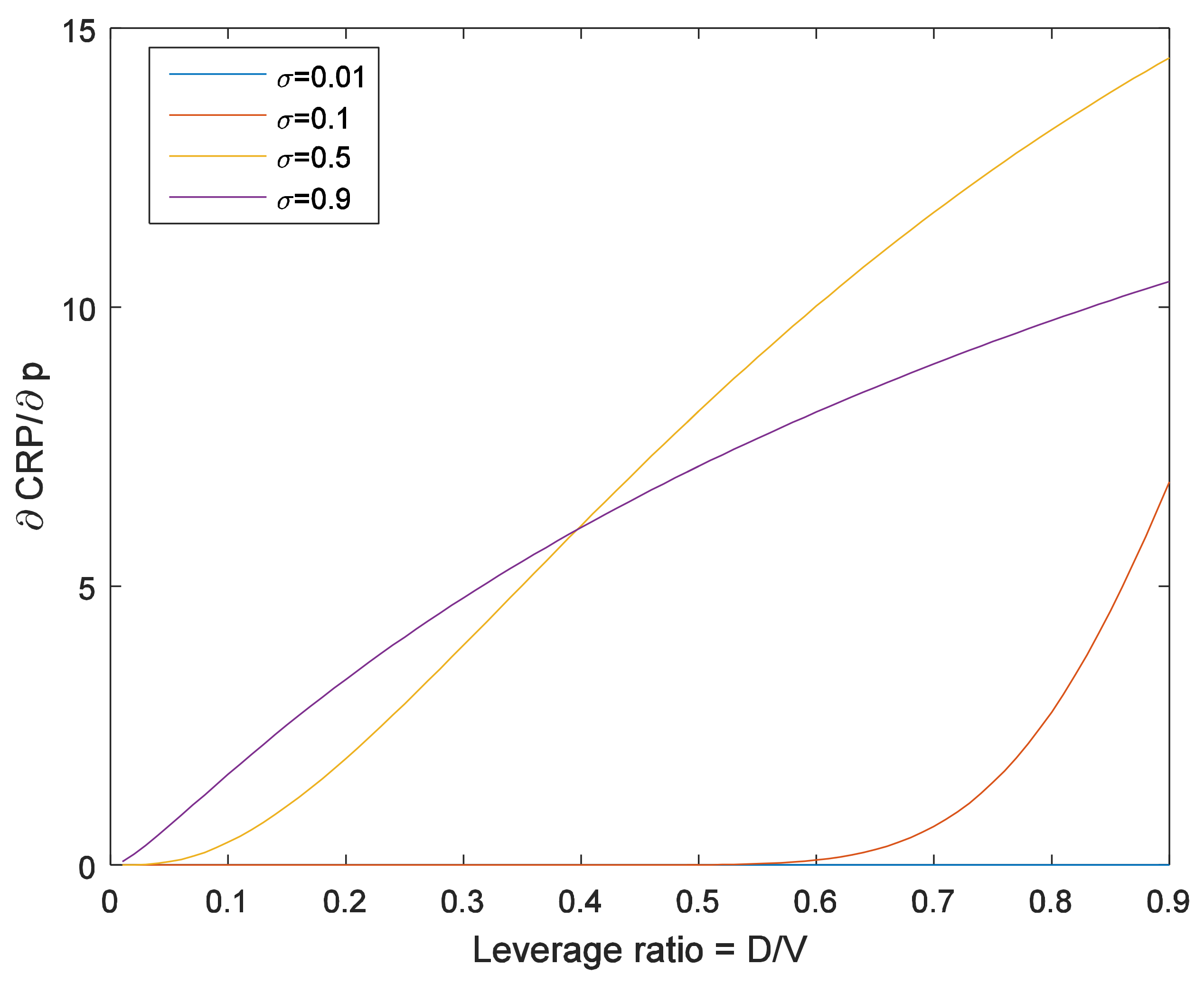
Figure 1 shows the effect of systematic default risk on CRPs depending on leverage ratio. Different curves correspond to different values of total risk $\sigma =\sqrt{{\beta }^2+{\gamma }^2}$. All graphs are plotted with a positive value of $\lambda$. We can see that, for reasonable values of the parameters, $\partial \mathrm{CRP}/\partial p$ is always positive when $\lambda$ is positive. Using the same logic, $\partial \mathrm{CRP}/\partial p$ is negative when $\lambda$ is negative. Based on this discussion, I develop the following hypothesis:

• “If the price of systematic asset risk is positive (negative), credit risk premiums will be higher (lower) for firms with higher systematic default risk after controlling for the total default risk.”

An important implication of this model is the fact that, even though the asset values of two firms are equally volatile, if one firm’s asset value (or default probability) is more sensitive to the systematic default risk that affects the entire economy, then investors request a higher premium for taking such credit risk, or CRP.

4. Methodology

This section describes how to estimate a CRP from a term-structure of corporate CDS spreads and how to decompose default risk into systematic and non-systematic components. The estimated CRPs are the dependent variable and the systematic default risk measures are the main independent variables that I focus on.

4.1. Independent Variable: Decomposition of Systematic Default Risk

I define systematic default risk as the default risk fluctuation arising from the systematic risk that affects all firms’ asset values as seen in Equation (9). In other words, the change in default probability (or change in asset value) owing to the systematic risk factor is the systematic default risk. Therefore, $\beta$ measures the systematic default risk. In the following subsections, I suggest how to estimate $\beta$.

4.1.1. Firm Value Beta Estimation

The purpose is to estimate how an asset value covaries with systematic risk factors or asset beta $\beta$. Estimating any beta between two time series is straightforward, but the difficulty in this case is that we cannot directly observe time series of asset values. To address this issue, I use the fact that a CDS spread is determined by a function of asset value dynamics.

$$ds=\left(\cdots \right)dt+\frac{\partial CDS}{\partial V}V\beta dF+\frac{\partial CDS}{\partial V}V\gamma dW$$

(12)

Given the CDS spreads and systematic risk factors data, we can estimate beta between CDS spreads and any factor, denoted by $b_S$. As systematic risk is independent of idiosyncratic risk, we see that $cov\left(dF,dW\right)=0$. This fact implies that $cov\left(ds,dF\right)=\frac{\partial CDS}{\partial V}V\beta var\left(dF\right)$. Therefore,

$$b_S\equiv \frac{cov\left(ds,dF\right)}{var\left(dF\right)}\approx \frac{\partial CDS}{\partial V}V\beta$$

(13)

Now I can compute asset beta implied in a CDS spread, $\beta$, from the CDS spread beta, $b_s$.

$$\beta ={\left(\frac{\partial CDS}{\partial V}\right)}^{-1}·\frac{b_s}{V}=-\frac{D}{V}·\frac{b_s}{N\left(-d_1\right)}$$

(14)

where $\frac{\partial CDS}{\partial V}=-N\left(-d_1\right)/D$ from Equation (6). The last work I need to do is estimate $N\left(-d_1\right)$ and $V$, which will be illustrated in the following section.

4.1.2. Distance-to-Default Estimation

To compute $\beta$, we need to estimate $d_1$ and current asset value $V$. Vassalou and Xing [20] suggested an algorithm for this estimation, which is most widely used by academics and in the finance industry (for example, references [21,22]). I also estimate these values by using the Vassalou and Xing algorithm, which I describe briefly here. For more details, refer to their paper.

Denoting current stock price of a firm by $E$, it can be expressed as

$$E=VN\left(d_1\right)-D{e}^{-rT}N\left(d_2\right),$$

(15)

under the assumptions made in the model setting section. The only unknown variables that we need to estimate are current asset value $V$ and asset volatility $\sigma =\sqrt{{\beta }^2+{\gamma }^2}$. Stock price $E$, default point $D$, and risk-free rates are observed in the market.

The first step of this algorithm is to solve the non-linear Equation (15) for current asset value $V$ with the historical volatility of stock returns as an initial value of $\sigma =\sqrt{{\beta }^2+{\gamma }^2}$. Then, I solve the equation for an updated value of the asset volatility ${\sigma }^{\prime }$ with V estimated in the previous step. I repeat this procedure and update V and $\sigma$ by the iterations until ${\mathsf{\sigma }}^{\prime }-\mathsf{\sigma }$ converges to some small tolerance level. I use the final values of V and $\sigma$ of the iterations as a proxy of current asset value and asset volatility. With these inputs, I evaluate $d_1$, which is often referred to as distance-to-default because default probability is low when $d_1$ is large, and $N\left(-d_1\right)$ meaning a probability of default.

4.2. Dependent Variable: Estimation of Credit Risk Premiums (CRPs)

To estimate the CRP implicit in the CDS term-structure, I follow the methodology introduced by Pan and Singleton [19]. First, I assume that the instantaneous credit spread or the intensity $\left({\lambda }^Q\right)$ of a point process determining the default of a firm follows a log normal process,

$$d\log {\lambda }^Q={\kappa }^Q\left({\theta }^Q-\log {\lambda }^Q\right)dt+\sigma d{W}_t^Q$$

(16)

where ${\kappa }^Q$, ${\theta }^Q$, and $\sigma$ are model parameters that determine the speed of mean-reversion, the long-run mean of the intensity, and the volatility of the log intensity, respectively. $W_t^Q$ is a standard Brownian motion. This type of process has a mean-reverting property that the log of intensity is forced to decrease (increase) when it is higher (lower) than the long-run mean. The rate of mean-reversion is determined by the level of $\kappa$. In addition, the intensity stochastically evolves by the random process $W_t^Q$ and the degree of the fluctuation (or volatility) is controlled by $\sigma$. Therefore, the change in log intensity in a very short period of time has a normal distribution. Another assumption I need to make is that the price of risk process is given by ${\alpha }_0+{\alpha }_1\log {\lambda }^Q$, which means that the price of intensity risk is proportional to the level of intensity. Under this price of risk setting, the dynamic of log intensity under a physical measure is linked by ${\kappa }^P={\kappa }^Q-{\alpha }_1\sigma$ and ${\kappa }^P{\theta }^P={\kappa }^Q{\theta }^Q+{\alpha }_0\sigma$.

An economic meaning of the intensity ${\lambda }^Q$ is the probability of default of a firm during a very short period of time. Thus, it also determines a firm’s default probability within an arbitrary period of time. The standard Brownian motion $W_t^Q$ drives the future uncertainty of the intensity, which implies that default probability is also risky, and investors request an additional premium for taking such risk. This premium is often called a credit risk premium (CRP) [12,13,19].

The technical procedure to estimate the model parameters is as follows. Based on these assumptions about the intensity and price of risk processes, the theoretical spread for a CDS with an arbitrary maturity of $T$ can be obtained by using a numerical method like the finite difference method, even though it is impossible to get a closed-form solution. Then, one can derive the likelihood of CDS spread data in hand from the fact that the intensity follows a log normal distribution. The empirical likelihood of CDS spreads can be evaluated once I extract out the intensity value implicit in a CDS spread by equating the model value with the observed value. Finally, I find the model parameters such as ${\delta }_0$, ${\delta }_1$, ${\kappa }^Q$, ${\theta }^Q$, and $\sigma$ that maximize the empirical likelihood. Throughout this procedure, I can estimate the model parameters and intensity. For more details on this procedure, please refer to Pan and Singleton [19].

Now, denoting the model spread with a maturity of $T$ at time $t$ as ${\mathrm{CDS}}_t^T$, I compute two types of model spreads. First, I evaluate the model spread function with Q-measure parameters like $CD{S}_t^T\left({\kappa }^Q,{\theta }^Q,\sigma \right)$. As I estimated the Q-measure parameters such that the model spread is the same as the observed spread, these computed model spreads are identical to actual market spreads. Next, I evaluate the model spread function with P-measure parameters, that is, $CD{S}_t^T\left({\kappa }^P,{\theta }^P,\sigma \right)$. This is not an actual spread, but it can be regarded as a spread without a risk premium. Pan and Singleton [19] defined this spread as “pseudo spread.” Finally, I compute the difference between the actual spread and the pseudo spread to compute the credit risk premium (CRP).

$$CRP\equiv \left[CD{S}_t^T\left({\kappa }^Q,{\theta }^Q,\sigma \right)-CD{S}_t^T\left({\kappa }^P,{\theta }^P,\sigma \right)\right]/CDS$$

(17)

Pan and Singleton [19] used this measure as the proxy of a credit risk premium, which makes sense because actual CDS spreads include a CRP, and the pseudo spread is, by definition, a pure component without the credit risk premium. Thus, the difference between the two spreads can be a proxy of the CRP. The reason that the premium is divided by CDS is to scale the value with respect to the current level of spread. This proxy of CRP is the main variable investigated in the regression analysis.

5. Empirical Tests

5.1. Raw Data

I collect data from a variety of data vendors. First, I obtain US corporate CDS spreads from Markit Group Limited (London, UK), a credit market data vendor. Markit provides corporate CDS spreads with various maturities. The data is reliable and has been used in many studies [23,24,25,26] since it is refined by smoothing quotes from more than two dealers. I use CDS spreads with a maturity of 1, 5, and 10 years. Second, I collect equity price data from the Center for Research in Security Prices (CRSP), and I use COMPUSTAT accounting information data. These data are collected via Warton Research Data Services (WRDS). The sample period is from January 2001 to November 2012. After cleaning the data, 664 firms were investigated in this study.

Table 1. Summary statistics of credit default swap (CDS) spreads across sectors (Panel A) and by ratings (Panel B).

	Mean			Max			Min			Std
	1Y	5Y	10Y	1Y	5Y	10Y	1Y	5Y	10Y	1Y	5Y	10Y
Panel A: Sector
None	143	156	164	1892	2149	1899	4	16	22	308	280	259
Fin	206	207	200	27,441	19,287	17,291	1	7	14	852	583	487
Ind	83	139	155	27,247	18,304	16,007	1	3	5	301	251	229
Tech	126	198	214	9834	6952	6608	1	5	7	364	339	299
CS	221	320	325	23,098	15,075	14,413	1	5	10	680	593	517
BM	132	189	207	35,637	19,384	16,841	1	9	15	768	497	429
CG	168	218	225	35,868	24,427	21,397	2	6	8	923	648	549
HC	66	124	142	1692	1526	1326	1	3	6	114	160	159
Eng	90	148	165	7280	5910	5900	1	2	5	291	271	247
Tel	200	313	325	6095	3996	3027	3	12	24	409	446	400
Uti	80	126	144	6871	3568	3611	2	10	23	208	171	160
Panel B: Rating
AAA	19	32	40	679	564	496	1	2	5	56	51	45
AA	28	43	52	1167	975	818	1	3	5	60	59	55
A	50	69	79	5805	3370	2576	1	4	8	169	126	106
BBB	73	110	126	7355	4307	3611	1	5	13	201	155	133
BB	175	269	285	17,550	9192	7647	1	19	22	372	322	279
B	407	546	538	12,098	8387	7228	2	13	20	858	687	583
CCC	990	926	846	35,868	24,427	21,397	3	11	19	3037	2019	1703
D	156	251	275	13,811	12,057	11,108	3	22	27	539	507	472
None	113	239	266	16,037	10,235	8479	2	10	13	366	322	291

Note: The sector name abbreviations are financials (Fin), industrials (Ind), technology (Tech), consumer services (CS), basic materials (BM), consumer goods (CG), health care (HC), energy (Eng), telecommunications (Tel), and utilities (Uti). 1Y, 5Y, and 10Y represent CDS maturities in year.

reports the summary statistics of CDS spreads across sectors (Panel A) and by ratings (Panel B). All spreads are measured in basis points. In terms of five-year maturity CDS, which is the most liquid contract, the spread of the consumer services (CS) sector was, on average, the highest in history (320 bp). The health care (HC) sector had the lowest level of CDS spread, with 124 bp. According to statistics by grade, the AAA average is 32 bp, and the CCC average is 926 bp. In the case of class D, the actual spread is rather low, since actual default events of D rating bonds are frequent.

On average, longer-term CDS spreads are higher than short-term ones over all sectors and all ratings, except the financial sector and rating B. In general, the CDS term structure exhibits an upward-sloping feature. Although not reported, during the financial crisis, the term structure was downward sloping. Except in such an extraordinary period, longer-term CDS spreads are higher at normal times.

5.2. Estimation of CRPs and Distance-to-default

Table 2. Estimated risk premium implicit in five-year CDS spreads.

	RP (bp)	CDS (bp)	LEV (%)	HVOL (%)
Mean	67.24	172.73	31.71	36.96
Std	874.38	208.13	20.73	17.31
Min	−3083.92	15.62	0.31	16.34
Max	14,477.76	2108.36	99.93	207.44
Skew	14.71	4.09	96.42	435.66
Kurt	236.46	26.36	61.09	3374.85

presents the estimation results of risk premiums using the Pan and Singleton model [19], along with firm characteristic structural variables such as leverage (LEV) and historical volatility (HVOL). LEV and HVOL are the main determinants of CDS spreads, as the Merton model suggests. In addition, empirical tests have shown that actual data evidence supports the theory. These two variables are used as a control variable in the regression analysis. The specific procedure of the estimation was provided in Section 4.2. The risk premium (RP) is the numerator of Formula (17), that is, $CD{S}_t^T\left({\kappa }^Q,{\theta }^Q,\sigma \right)-CD{S}_t^T\left({\kappa }^P,{\theta }^P,\sigma \right)$. Leverage (LEV) was computed as the default point divided by the sum of the default point and the total market value of equity including both common and preferred stocks. That is, the LEV ratio measures the degree of debt compared to the asset value of a firm. Historical volatility (HVOL) of a firm is the standard deviation of one-year past stock returns.

Several results are noteworthy. First, while the average CDS spread is around 173 bp, the CRP in the spread is about 67 bp on average. Thus, CRP, which is the ratio of RP to CDS, is approximately 38.93% on average. In other words, the RP component accounts for around 38.93% of a CDS spread for US firms. Second, the average leverage ratio is approximately 32%, implying that the default debt point is at a 32% level of the current asset value. If the asset value drops by 68%, the firm will suffer from insolvency of the debt. Also, we can see that there is a firm that has little debt (min = 0.31%) and whose asset value is almost free from debt (max = 99.93%). Third, annualized HVOL is 37% on average, while the minimum is 16% and the maximum is 207%.

Table 3. Results of distance-to-default estimation.

	Market Equity ($millions)	Default Point ($millions)	Default Probability	σ
Mean	14,164	5.64	0.08	0.43
Std	31,907	33.82	0.14	0.20
Min	56	0.00	0.00	0.08
Max	350,620	583.86	0.89	1.87
Skew	5	12.34	2.49	2.40
Kurt	38	175.50	6.99	10.12

reports the estimation results associated with distance-to-default. The algorithm was provided in Section 4.1.2. The distance-to-default ($d_1$) and default probability $N\left(-d_1\right)$ are computed for one-year maturity. Therefore, $N\left(-d_1\right)$ implies the probability of defaulting in one year. Note that this probability is not actual probability but risk-neutral probability, as I evaluated with the risk-free rate rather than the expected rate of asset growth. For this reason, Vassalou and Xing [20] called this the “default likelihood indicator.” In my study, it is not necessary to estimate the physical default. Therefore I simply use the term of (risk-neutral) default probability. Average probability to default in one year is 8% for US firms. The maximum default probability is 89% and the minimum default probability is nearly 0% which may correspond to the firm with nearly zero debt. I also report the asset volatility estimation result in the last column. On average, asset volatility (43%) in Table 3 is higher than the HVOL of stock returns (37%) reported in Table 2.

5.3. Systematic Factors in the CDS Market

To investigate what determines CDS spreads and what might be systematic risk, I run the regression method used by Collin-Dufresne et al. [8] and Ericsson et al. [9]. The specific procedure is as follows. I run the following time-series regression for each firm:

$$\Delta s_t={\alpha }_0+{\alpha }_1\Delta F_t+\alpha \Delta X_t+{\epsilon }_t$$

(18)

where $s_t$ is a CDS spread observation of a firm, $F_t$ is a systematic risk factor such as market-wide average CDS level (MCDS) and market-wide average CDS slope ($MSLOPE$), and $X_t$ is a control variable such as $LEV$ and $HVOL$. The CDS slope is measured by the difference between the five-year and one-year spreads. The notation $\Delta$ denotes the time change in a variable. After conducting this regression for every firm, I compute the cross-sectional average of each coefficient to construct a point estimate of the regression. Corresponding t-statistics are computed by the point estimate divided by its standard error across each regression coefficient.

Table 4. Effect of risk factors on CDS spreads.

Explanatory Variables	M1	M2	M3	M4	M5	M6
Intercept	0.00	0.03 ***	0.00 ***	−0.02 ***	−0.02 ***	−0.02 ***
	(0.31)	(10.86)	(2.65)	(−3.71)	(−3.10)	(−3.11)
MCDS	1.13 ***		1.01 ***	0.79 ***		0.64 ***
	(7.23)		(7.82)	(4.99)		(7.04)
MSLOPE		−1.04 ***	−0.23 *		−0.84 **	−0.46
		(−5.75)	(−1.89)		(−2.05)	(−1.25)
LEV				0.03 **	0.07 ***	0.04 ***
				(2.31)	(9.28)	(3.29)
HVOL				0.01 ***	0.03 ***	0.02 **
				(4.10)	(3.40)	(2.40)
N	664	664	664	664	664	664
Adj.R2	0.41	0.21	0.55	0.65	0.59	0.71

Note: Adj.R2 represents the average adjusted R-squared of time-series regressions of all firms. N denotes the number of firms analyzed. ***, **, and * correspond to 1%, 5%, and 10% significance levels, respectively.

reports the results. The t-statistics are in parentheses below the point estimates. In M1, the average level of CDS spreads in the market is used as a systematic risk factor $F$. The reason for this selection is that market-wide average CDS spread (MCDS) is high when the entire market suffers from high default probability. The underlying risk factor affecting MCDS is likely to affect almost all firms’ default probability. Thus, MCDS can be a proxy of systematic default risk. As shown, the change in MCDS is indeed positively associated with the change in a CDS spread, suggesting that individual firms’ default probability is likely to be high when the overall market condition is bad. The result is statistically significant, which implies that the effect of MCDS on an individual CDS spread is reliably similar across firms because a large t-statistic means a small variation across firms. Therefore, we can see that MCDS is consistent with the definition of a systematic default risk factor.

M2 tests if the market-wide CDS term-structure (MSLOPE) is a determinant of individual CDS spreads. The result reveals that MSLOPE negatively drives CDS spreads. In other words, if the market-wide slope becomes rather flat or highly downward-sloping, CDS spreads tend to increase and individual firms’ default probability increases. This is consistent with empirical evidence that during the recent global crisis period, the overall market CDS slope was downward-sloping and many firms suffered from the likelihood of bankruptcy.

Even though MCDS and MSLOPE are significant determinants of individual CDS spreads in the respective univariate regressions (M1 and M2), MSLOPE becomes marginally significant when MCDS is used together as a regressor, whereas MCDS is still very significant in the multivariate regression (see M3). In addition, MCDS remains significant even after controlling for the Merton model variables such as LEV and HVOL. These results imply that MCDS is a more influential systematic default risk factor.

5.4. Effect of Systematic Default Risks on CRPs

Now I test my main hypothesis as to whether the market price of risk positive (negative) CRPs is higher (lower) for firms with higher systematic default risk. To this end, I run the Fama-MacBeth regression [27]. The dependent variable of the regression is an individual firm’s CRP, and the independent variables are the systematic default risk measures that are estimated by a factor loading as described in the method described in Section 4.1.1. I select five factor candidates based on the analysis in the previous section and the results of the literature. First, I chose the MCDS and the market-wide average CDS slope (MSLOPE) for the testing factors. These two factors were obtained from the credit market and thus, can be a rather direct measure of systematic default risk. In addition, I also chose Fama-French three factors [28,29,30] such as excess market return (MKT), size risk factor (SMB), and value risk factor (HML) as equity market risk factors. Including Fama and French [28,29,30], a significant number of papers have reported that these three factors are systematic risk factors in the equity market. These factors can also affect asset values and default probability for all firms. Using these factors, I compute the systematic default risk measures (asset betas in Equation (14)), denoted by ${\beta }_{MCDS}$, ${\beta }_{MSLOPE}$, ${\beta }_{MKT}$, ${\beta }_{SMB}$, and ${\beta }_{HML}$.

The Fama-MacBeth type regression is conducted as follows. First, in each month, I run a cross-sectional regression using individual firms’ CRP as the dependent variable and systematic default risk measures (asset betas) as the independent variables. The reason why I use CRP rather than risk premium is to address endogeneity issues. CRP is a risk premium normalized by the level of CDS spread. Repeating this process over the sample period every month, I obtain a time series of respective regression coefficients for each of the systematic default risk measures. Second, I compute the average value of the time series of regression coefficients to estimate a point estimator for the cross-sectional relation between CRP and the systematic default risk measures.

Table 5. Results of Fama-MacBeth regressions of the credit risk premium.

	M1	M2	M3	M4	M5
Intercept	1.488 ***	1.348 ***	1.631 ***	2.056 ***	2.116 ***
	(4.66)	(4.60)	(4.72)	(4.04)	(3.97)
${\beta }_{MCDS}$	0.033 **		0.060 **		0.040 **
	(2.47)		(2.18)		(2.22)
${\beta }_{MSLOPE}$		−0.011	0.013		0.007
		(−0.99)	(0.77)		(0.61)
${\beta }_{MKT}$				−0.679 *	−0.525
				(−1.78)	(−1.43)
${\beta }_{SMB}$				−0.254 *	−0.212
				(−1.68)	(−1.41)
${\beta }_{HML}$				−0.387 ***	−0.367 ***
				(−3.85)	(−3.49)
Adj.R2	0.003	0.002	0.005	0.007	0.012

Note: Adj.R2 represents the average adjusted R-squared of monthly cross-sectional regressions. All t-statistics in parentheses are adjusted by the Newey-West method [31]. ***, **, and * correspond to 1%, 5%, and 10% significance levels, respectively.

reports the average estimates and their corresponding t-statistics in parentheses.

Some interesting findings are summarized as follows. First, M1 proves that the MCDS is a systematic default risk and it increases a CRP at a meaningful statistical significance level. This is consistent over all regression models regardless of the inclusion of other risk factors. Second, the market-wide average CDS slope is not significantly priced in the cross section of CRPs. In the previous tests in Table 4, the CDS spread loading to the market CDS slope, $b_s\left(MSLOPE\right)$, explained the cross section of CDS spreads. However, asset beta with respect to the market-wide slope factor cannot explain CRPs. To sum up, among credit market factors, the average level of CDS spreads is the only priced factor, while the “value” risk factor is the only priced factor among equity market factors.

One noticeable result is the sign of regression coefficients, especially for MCDS and HML factors. The sign of $\partial \mathrm{CRP}/\partial p$ is identical to the sign of $\mathsf{\lambda }$. Therefore, in the empirical results, a positive (negative) regression coefficient implies that the market price of the risk is positive (negative). This indicates that investors dislike holding assets with high sensitivity to overall market default likelihood (MCDS) and will request a positive risk premium. In contrast, the negative market price of risk for HML implies that investors prefer high sensitivity to value factor (HML). The reason for such a preference could be hedge demand. By holding assets with high loading to HML, investors may be able to hedge the systematic default risk.

The opposite effects of credit and equity market risk factors on CRP can be partly understood in view of the Black-Scholes option pricing theory [17]. As explained earlier, credit spreads can be viewed as a put option written on asset value. At the same time, equity price can also be viewed as a call option written on the asset value [7,13,22]. By the put-call parity [32], it is necessary for the prices of the two options to move in an opposite direction. As shown in empirical factor pricing model studies, individual stock prices are significantly influenced by equity market factors [28,29,30], and Table 4 shows that credit spreads are influenced by credit market factors. With the notion that credit spreads and stock prices are inversely related by the put-call parity argument, the opposite effects of credit and equity market risk factors on CRP can be reconciled with the option pricing theory.

Finally, the empirical result show that equity market factors (MKT, SMB, and HML) can explain the cross section of CRPs better than credit market factors (MCDS and MSLOPE), in terms of adjusted R-squared. While M3 shows that credit market factors have an explanatory power of 0.5%, M4 exhibits equity market factors as having an explanatory power of 0.7%. Some might criticize the degree of the explanatory power as being too weak, which is very common in cross-sectional regressions of individual assets in finance literature (see, e.g., Hou and Loh [33]). This is mainly because individual stock return data is very noisy. One way of addressing this issue is to construct portfolios and compute their returns so that the noise can be averaged out in the portfolio return computation. When portfolios rather than individual stocks are tested, the explanatory power increases (see, e.g., Fama and French [30]). Although not reported, this is the case in this study. However, the main purpose of the study was not to find the model that can best explain the cross section of CRPs. Rather, I focus on testing if systematic default risk is priced into CRPs. Thus, I pay attention to the significance of the coefficients rather than the explanatory power of the regression model, which is a typical practice in the empirical asset pricing studies [34].

Even though some of the results at this stage are somewhat puzzling, I will show, in the next analysis, that the effect of equity market factors is mostly because of the association with CDS determinants such as LEV and HVOL. After controlling for these effects, credit market factors are more influential on systematic default risk factors than are equity market factors.

I repeat the same analysis with control variables such as leverage ratio and historical volatility. The reason that I control for leverage and historical volatility is to address the endogeneity issue that they are known as the determinants of credit spreads or CDS spreads. This is true both theoretically and empirically. The Merton model tells us that two important determinants are leverage ratio and volatility of asset value. Many previous papers [8,9,10] have shown that these two variables are important to explain the time-series fluctuation of CDS spreads. I also confirmed this fact in Table 4. For this reason, if these variables determine the level of CDS spreads, they can subsequently affect CRPs. Therefore, we need to control for such an effect. Another reason for the volatility control is to control for the total risk of asset value or default. The main hypothesis is developed under the condition where the total variation of asset value is constant, and I need to examine if CRPs are positively associated with systematic default risk after controlling for the total default risk, the sum of systematic and idiosyncratic components. To this end, I use historical volatility as a proxy of the total risk.

In

Table 6. Results of Fama-MacBeth regressions of the credit risk premium with controls.

	M1	M2	M3	M4	M5
Intercept	4.511 ***	4.538 ***	4.572 ***	4.604 ***	4.691 ***
	(6.08)	(6.02)	(6.04)	(6.43)	(6.41)
${\beta }_{MCDS}$	0.025 **		0.042 **	0.023 **	0.037 **
	(2.10)		(2.13)	(2.04)	(2.15)
${\beta }_{MSLOPE}$		−0.010	0.005		0.009
		(−1.02)	(0.36)		(0.78)
${\beta }_{MKT}$				−0.175	−0.126
				(−0.38)	(−0.26)
${\beta }_{SMB}$				−0.027	−0.009
				(−0.14)	(−0.04)
${\beta }_{HML}$				−0.225 *	−0.219 *
				(−1.75)	(−1.69)
LEV	−6.937 ***	−6.929 ***	−6.972 ***	−7.187 ***	−7.213 ***
	(−6.20)	(−6.09)	(−6.09)	(−6.36)	(−6.23)
HVOL	−3.728 ***	−4.125 ***	−3.651 ***	−2.985	−3.170
	(−3.01)	(−3.41)	(−3.10)	(−1.39)	(−1.46)
Adj.R2	0.019	0.019	0.022	0.026	0.029

Note: Adj.R2 represents the average adjusted R-squared of monthly cross-sectional regressions. All t-statistics in parentheses are adjusted by the Newey-West method [31]. ***, **, and * correspond to 1%, 5%, and 10% significance levels, respectively.

, I confirm that the main result remains the same even after controlling for CDS determinants and a total risk proxy. M1 shows that the average market CDS level is positively priced in CRPs after controlling for total risk. This result is very robust over all models with other variables. Similar to the previous results, the average market CDS slope has mostly a positive effect on CRPs when including other risk factors in the regression, while its effect is negative when it is solely used as a risk factor with controls (M2). However, the MSLOPE effect is not statistically significant.

Equity market risk factors show similar results to the findings of tests without controls. One exception is HML. When control variables were not used earlier, HML was highly statistically significant in Table 5. However, the significance mitigates and is now marginally significant even though the sign is still negative. It seems that the effect of HML is subsumed by the effect of the leverage ratio. Generally, firms with a high leverage ratio exhibit high loading to the HML factor. The two effects are positively associated. The negative effect of leverage on CRPs is much stronger than the negative effect of the HML risk factor, and this leverage effect subsumes part of the HML effect. Similarly, the MKT effect is subsumed by the HVOL effect because historical volatility of an individual firm is highly associated with stock market risk.

Consistent with this reason, I argue that credit market factors (MCDS and MSLOPE) are more influential than equity market factors (MKT, SMB, and HML). M3 shows that the explanatory power of credit market factors with controls is 2.2%, but in M5, the inclusion of equity market factors seldom increases the power. The increment is only 0.7%, and this is because the source of the strong effect of equity market factors is the CDS determinants (LEV and HVOL).

To summarize, even after controlling for total risk and leverage ratio, systematic default risk is positively associated with CRPs when the market price of risk is positive. Also, credit market risk factors are much stronger than equity market risk factors for CRPs.

6. Conclusions

This study examines the effect of systematic default risk on a cross section of credit risk premiums. Based on the Merton model assumptions, I developed a testable hypothesis that firms with higher systematic default risk tend to have higher CRPs when the market price of the risk is positive. The sign of this relation depends on the sign of the market price of risk.

The findings show that the well-known systematic risk factors in the stock market affect a cross section of credit risk premiums. I also find that two additional systematic default risk factors, obtained from credit markets (market average CDS level and its slope), are associated with a cross section of credit risk premiums. Interestingly, credit market factors are more influential than stock market factors. Finally, while credit market factors are positively priced, stock market factors are negatively priced.

Among the factors tested, the most significant factor is the market’s average CDS level, which has a positive impact on the cross section of the CRPs and maintains its statistical significance even after controlling for various factors. This finding implies that the greater the risk exposure to the market’s average default risk, the higher the percentage of CRPs in CDS spreads.

The empirical findings imply that even when total default risk is the same for two firms, investors request a higher premium for the firm with a higher systematic default risk component. Considering that CDS spreads are a proxy for credit spreads that increase a firm’s cost of capital, in addition to risk-interest costs, a firm’s manager should focus on managing exposure to the systematic default risk to reduce its cost of capital. If a firm’s assets have more exposure to the HML risk factor, there is a smaller credit risk premium in its credit spread when the expected rate of default remains the same. This will reduce the credit spread and subsequently, the cost of capital. In contrast, all else being equal, financial managers need to pay attention to the management of the covariance of asset risk with market-wide credit risk. Even if the expected default probability is the same, the cost of capital (or a CDS spread) can be high because of the increase in CRP.

A future direction for this study could be to test more specific risk factors in the credit market. For example, while I measured the overall credit market risk using the average level of CDSs, the impact of investment-grade and speculative-grade CDSs may be different because the two credit markets are separate. I leave this issue for future work.

References

- Stulz, R.M. Credit Default Swaps and the Credit Crisis. J. Econ. Perspect. 2010, 24, 73–92. [Google Scholar] [CrossRef] [Green Version]
- Anderson, M. Contagion and Excess Correlation in Credit Default Swaps; Social Science Research Network: Rochester, NY, USA, 2011. [Google Scholar]
- Benzoni, L.; Collin-Dufresne, P.; Goldstein, R.S.; Helwege, J. Modeling credit contagion via the updating of fragile beliefs. Rev. Financ. Stud. 2015, 28, 1960–2008. [Google Scholar] [CrossRef]
- Collin-Dufresne, P.; Goldstein, R.S.; Helwege, J. Is Credit Event Risk Priced? Modeling Contagion via the Updating of Beliefs; National Bureau of Economic Research: Cambridge, MA, USA, 2010. [Google Scholar]
- Lando, D.; Nielsen, M.S. Correlation in corporate defaults: Contagion or conditional independence? J. Financ. Intermed. 2010, 19, 355–372. [Google Scholar] [CrossRef]
- Kenourgios, D.; Dimitriou, D. Contagion of the Global Financial Crisis and the real economy: A regional analysis. Econ. Model 2015, 44, 283–293. [Google Scholar] [CrossRef]
- Merton, R.C. On the pricing of corporate debt: The risk structure of interest rates. J. Financ. 1974, 29, 449–470. [Google Scholar]
- Collin-Dufresne, P.; Goldstein, R.S.; Martin, J.S. The determinants of credit spread changes. J. Financ. 2001, 56, 2177–2207. [Google Scholar] [CrossRef]
- Ericsson, J.; Jacobs, K.; Oviedo, R. The determinants of credit default swap premia. J. Financ. Quant. Anal. 2009, 44, 109–132. [Google Scholar] [CrossRef]
- Galil, K.; Shapir, O.M.; Amiram, D.; Ben-Zion, U. The determinants of CDS spreads. J. Bank. Financ. 2014, 41, 271–282. [Google Scholar] [CrossRef] [Green Version]
- Berndt, A.; Douglas, R.; Duffie, D.; Ferguson, M. Corporate credit risk premia. Rev. Financ. 2018, 22, 419–454. [Google Scholar] [CrossRef]
- Díaz, A.; Groba, J.; Serrano, P. What drives corporate default risk premia? Evidence from the CDS market. J. Int. Money Financ. 2013, 37, 529–563. [Google Scholar] [CrossRef] [Green Version]
- Friewald, N.; Wagner, C.; Zechner, J. The Cross-Section of Credit Risk Premia and Equity Returns. J. Financ. 2014, 69, 2419–2469. [Google Scholar] [CrossRef] [Green Version]
- Campbell, J.Y.; Hilscher, J.; Szilagyi, J. In Search of Distress Risk. J. Financ. 2008, 63, 2899–2939. [Google Scholar] [CrossRef] [Green Version]
- George, T.J.; Hwang, C.-Y. A resolution of the distress risk and leverage puzzles in the cross section of stock returns. J. Financ. Econ. 2010, 96, 56–79. [Google Scholar] [CrossRef]
- Huang, J.-Z.; Huang, M. How Much of the Corporate-Treasury Yield Spread Is Due to Credit Risk? Rev. Asset Pricing Stud. 2012, 2, 153–202. [Google Scholar] [CrossRef] [Green Version]
- Black, F.; Scholes, M. The pricing of options and corporate liabilities. J. Polit. Econ. 1973, 637–654. [Google Scholar] [CrossRef]
- Carr, P.; Wu, L. Stock options and credit default swaps: A joint framework for valuation and estimation. J. Financ. Econ. 2010, 8, 409–449. [Google Scholar] [CrossRef]
- Pan, J.; Singleton, K.J. Default and recovery implicit in the term structure of sovereign CDS spreads. J. Financ. 2008, 63, 2345–2384. [Google Scholar] [CrossRef]
- Vassalou, M.; Xing, Y. Default Risk in Equity Returns. J. Financ. 2004, 59, 831–868. [Google Scholar] [CrossRef]
- Bharath, S.T.; Shumway, T. Forecasting default with the Merton distance to default model. Rev. Financ. Stud. 2008, 21, 1339–1369. [Google Scholar] [CrossRef]
- Gilchrist, S.; Zakrajšek, E. Credit Spreads and Business Cycle Fluctuations. Am. Econ. Rev. 2012, 102, 1692–1720. [Google Scholar] [CrossRef]
- Fender, I.; Hayo, B.; Neuenkirch, M. Daily pricing of emerging market sovereign CDS before and during the global financial crisis. J. Bank. Financ. 2012, 36, 2786–2794. [Google Scholar] [CrossRef]
- Griffin, P.A.; Hong, H.A.; Kim, J.-B. Price discovery in the CDS market: The informational role of equity short interest. Rev. Account. Stud. 2016, 21, 1116–1148. [Google Scholar] [CrossRef]
- Hilscher, J.; Pollet, J.M.; Wilson, M. Are Credit Default Swaps a Sideshow? Evidence That Information Flows from Equity to CDS Markets. J. Financ. Quant. Anal. 2015, 50, 543–567. [Google Scholar] [CrossRef] [Green Version]
- Oehmke, M.; Zawadowski, A. The anatomy of the CDS market. Rev. Financ. Stud. 2016, 30, 80–119. [Google Scholar] [CrossRef]
- Fama, E.F.; MacBeth, J.D. Risk, return, and equilibrium: Empirical tests. J. Polit. Econ. 1973, 607–636. [Google Scholar] [CrossRef]
- Fama, E.F.; French, K.R. Common risk factors in the returns on stocks and bonds. J. Financ. Econ. 1993, 33, 3–56. [Google Scholar] [CrossRef]
- Fama, E.F.; French, K.R. Multifactor Explanations of Asset Pricing Anomalies. J. Financ. 1996, 51, 55–84. [Google Scholar] [CrossRef]
- Fama, E.F.; French, K.R. A five-factor asset pricing model. J. Financ. Econ. 2015, 116, 1–22. [Google Scholar] [CrossRef] [Green Version]
- Newey, W.; West, K. A Simple, Positive Semi-Definite, Heteroskedasticity and Autocorrelation Consistent Covariance Matrix. Econometrica 1987, 55, 703–708. [Google Scholar] [CrossRef]
- Cremers, M.; Weinbaum, D. Deviations from Put-Call Parity and Stock Return Predictability. J. Financ. Quant. Anal. 2010, 45, 335–367. [Google Scholar] [CrossRef] [Green Version]
- Hou, K.; Loh, R.K. Have we solved the idiosyncratic volatility puzzle? J. Financ. Econ. 2016, 121, 167–194. [Google Scholar] [CrossRef]
- Linnainmaa, J.T.; Roberts, M.R. The History of the Cross-Section of Stock Returns. Rev. Financ. Stud. 2018, 31, 2606–2649. [Google Scholar] [CrossRef] [Green Version]
Figure 1.
Effect of systematic default risk on credit risk premiums (CRPs) depending on leverage ratio. Different curves correspond to the different values of total risk .