Article

Flights Dominate Travel Emissions of Young Urbanites

by
Michał Czepkiewicz
*,
Áróra Árnadóttir
and
Jukka Heinonen
Faculty of Civil and Environmental Engineering, University of Iceland, 107 Reykjavík, Iceland
*
Author to whom correspondence should be addressed.
Sustainability 2019, 11(22), 6340; https://doi.org/10.3390/su11226340
Submission received: 13 September 2019 / Revised: 31 October 2019 / Accepted: 6 November 2019 / Published: 12 November 2019
(This article belongs to the Section Sustainable Transportation)

Abstract

:
Transport is a key sector in reducing greenhouse gas (GHG) emissions. A consensus prevails on a causal relationship between distance to the city center and emissions from private transport, which has led to an emphasis on density in urban planning. However, several studies have reported a reverse association between the level of urbanity and emissions from long-distance leisure travel. Studies have also suggested that pro-environmental attitudes and climate change concerns are unrelated or positively related to emissions from long-distance travel. The goals of this case study were to find out the structure, levels, distribution, and predictors of GHG emissions from the local, domestic, and international travel of young adults of the Reykjavik Capital Region. A life cycle assessment (LCA) approach was utilized to calculate emissions, and the materials were collected with a map-based online survey. International leisure travel dominated the overall GHG emissions from personal travel regardless of residential location, modality style, or income level. A highly unequal distribution of emissions was found. A higher climate change awareness was found to predict higher GHG emissions from trips abroad. Emissions from leisure travel abroad were the highest in the city center, which was related to cosmopolitan attitudes among downtown dwellers.

1. Introduction

A record amount of 42 Gt of CO2 was emitted in 2017 [1]. The amount of carbon that can be safely emitted without reaching 1.5-degree warming (i.e., global carbon budget) can be as low as 420 GtCO2-eq. [2], just ten times the current annual emissions. Higher budget estimations have been presented as well [3,4], but it is evident that rapid and deep emission cuts need to take place, even if the aim is to avoid 2-degree warming [2]. At the same time, emissions have not turned down and are still on an upward path [1].
Transport is one of the key sectors, as it causes over 20% of the global greenhouse gas (GHG) emissions [1] and is also a sector where the emissions are growing. Electrification and the development of other alternative power sources are likely to lead to a reduction in the emissions from the transport sector, but structural changes, such as improving the efficiency of freight [5], reducing travel demand, and modal shifts to low-carbon modes, may be necessary to reach deeper mitigation [1].
Several studies focusing on private transport and local travel have generally concluded that distance to the city center and other urban form characteristics correlate with car use, vehicle distances traveled, and emissions [6,7,8,9]. Despite continuing “chicken or the egg” debates, e.g., on residential self-selection [10], the link has an established causal character [11,12]. Despite this, land-use and transport planning may not be the most effective or sufficient strategies for mitigating emissions from transportation [13]. Emissions have been growing because of other factors, largely unrelated to urban planning, such as the globalization of social networks and businesses.
One such aspect is the growth in long-distance travel and particularly aviation. GHG emissions from aviation are estimated only at 2%–3% of the total global GHG emissions, but they are growing faster than those from the transport sector overall [1] and are estimated to reach 20% of global emissions by 2050 without mitigating action [14]. The percentages are also significantly higher in wealthy societies, such as Nordic and other European countries [15,16,17]. The role of aviation is especially significant when including short-lived climate forcers. If developed and wealthy societies of the North are seriously thinking about climate change mitigation, they need to address the aviation of their members. Studying predictors and contradictions related to long-distance travel behaviors may help create more effective policies.
Multiple studies in highly mobile societies have reported a positive association between the level of urbanity and the amount of long-distance travel [18]. There is no academic consensus on how long-distance travel connects to the urban form, but some of findings have suggested that the emissions from long-distance travel, particularly from aviation, might work towards negating the GHG reductions in local travel resulting from urban densification. A related body of literature has shown that pro-environmental and climate change-related attitudes are unrelated or positively related to emissions from long-distance travel and tourism [19]. The article focuses on these two contradictions.

1.1. The First Contradiction: Emissions from Long-Distance Travel Higher in Cities and City Centers

Previous studies have suggested that the frequency and carbon impact of long-distance travel and particularly leisure flights is higher among residents of bigger cities than residents of smaller settlements (e.g., [20]). Multiple studies have also suggested that within cities, residents of urban cores fly more than residents of suburbs [17,18]. When total travel GHG emissions have been compared (including local travel), their levels have been found to be similar in different kinds of settlements and urban areas [8,17,20].
Differences in sociodemographic and economic characteristics explain the geographical patterns to some extent. Flights are highly elastic, and higher incomes are related to more flights [21]; there are, in many places, income differences between and within settlements. Family type, particularly having children, also affects leisure mobility [22], and in many cities, single people and childless couples tend to live in city centers, which may explain part of the geographical variation. However, in many studies, these variables are controlled for, and still, residential location is a strong predictor of the number of flights and related emissions. Therefore, other explanations are necessary.
The compensation hypothesis related to recreational opportunities in dense cities [23,24,25,26], travel-cost rebound effects related to car ownership [8,27], access to travel infrastructure, e.g., airports [28], the dispersion of social networks [20,29,30], and the cosmopolitan attitudes and lifestyles [23,31] of urban populations have been suggested as the potential explanations. How much and under which conditions these different explanations apply remains not fully understood, and room exists for their empirical verification. Previous studies have rarely jointly considered residential location and various socio-cultural and psychological factors, such as cosmopolitan attitudes or language skills. This study contributes to filling the gap in understanding how the residential location and geographical sorting of residents influence emissions from travel.

1.2. The Second Contradiction: Environmental Concern Unrelated or Positively Related to Flights and Emissions

Awareness of and concern with environmental burdens caused by human activity does not always translate into lower emissions, indicating that the existence of an awareness–attitude–behavior gap, which manifests in a way that values, beliefs, or norms do not translate into actions or behaviors. This gap has been extensively studied with varying results; many have found the connection to be non-existent or weak [32,33,34,35,36,37], but in some cases, environmental attitude has been found to be related to lower impacts in categories such as diet, energy use and local travel emissions [38,39,40].
When it comes to air travel, the inconsistency between attitudes and air travel behavior is especially prominent and has been found in several studies [19,41,42]. It seems that people are not willing to alter their air travel behavior to match their environmental concerns, although they may have a “green” lifestyle around the home and even use their local green behavior to justify their long-distance travel [43,44,45]. Instead of considering the sum of impacts an individual’s lifestyle has on the environment, it is common for one to think that they have an average impact, thus creating an illusion of a low-carbon lifestyle [46].
Some barriers to the discrepancies between environmental concern and holiday travel have been identified and include, for example, a lack of other available options [35] and the importance of long-distance travel for well-being and social status [47,48]. This study analyzes how climate change awareness interacts with other variables and influences emissions from travel in one affluent and remote urban region and suggests some novel explanations.

1.3. Research Goals and Questions

The study was conducted to improve the state-of-the-art in the context of emissions from long-distance travel in comparison to those from local transport, reasons for variation in travel activity, the impact of geographic location, and the qualities of the surrounding urban structure. It was conducted in the Reykjavik Capital Region (Reykjavik), which offered an interesting case due to the isolated northern location of Iceland with few alternatives to flying for traveling abroad, the high affluence of the residents, and easy access to a well-connected international airport. The residents of Reykjavik are also, on average, highly language-skilled.
The goals of the study were to find out:
  • The structure of GHG emissions from travel in the Reykjavik Capital Region (Reykjavik) in Iceland
    a.
    The distribution of emissions among the studied population.
    b.
    The levels of emissions from local, domestic and international travel.
    c.
    The geographical distribution of emissions within an urban region based on residential location.
  • Factors that influence this structure, specifically focusing on the contradictions described above:
    a.
    How does residential location within the urban region influence emissions from travel?
    b.
    How does awareness of climate change influence emissions from travel?
    c.
    What are other factors that influence the amount of travel-related emissions?
We utilized a wide-scope life cycle assessment (LCA) approach, capturing not only the direct emissions but also the indirect emissions from fuel production, vehicle manufacturing, and infrastructure construction, suggested as important contributors to the emissions from travel [49]. For aviation, we included the short-lived climate forcers. We also report the breakdown of the emissions to the direct and indirect components, which has rarely been done in previous studies. The study materials were collected with a map-based online survey (a soft geographical information system (softGIS) survey or a geo-questionnaire), distributed among young adults living in Reykjavik in fall 2017. The following section provides a more detailed description of the methods and materials used in the study.

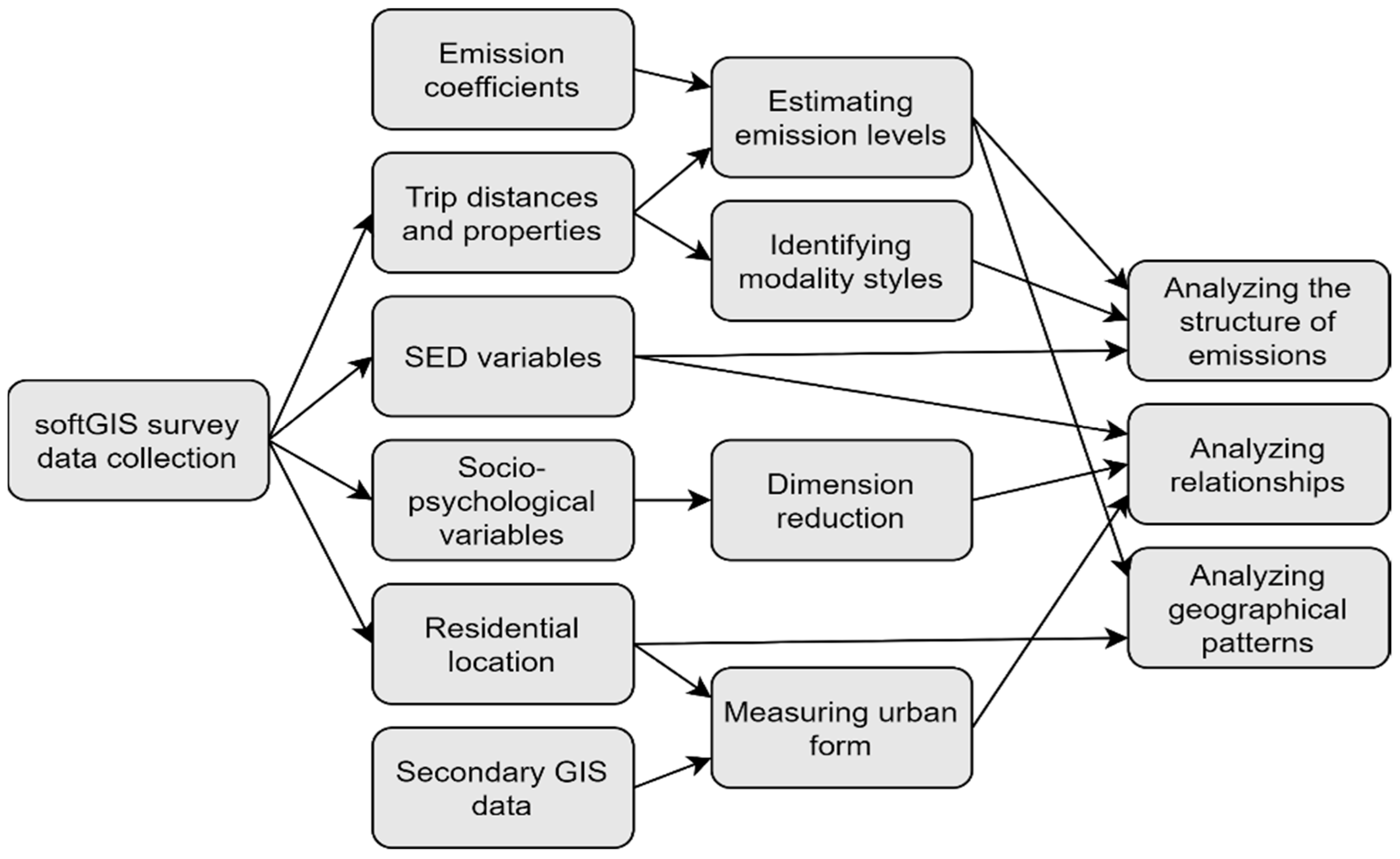
2. Materials and Methods

2.1. Case Area

The data were collected from the residents of the Reykjavík Capital Region (Höfuðborgarsvæðið), including the municipalities of Reykjavík, Kópavogur, Hafnarfjörður, Garðabær, Mosfellsbær, Seltjarnarnes, and Kjósarhreppur. The population of the region is just under 230,000 [50], which constitutes around 65% of the country’s population. Compared to other Nordic cities, the urban structure of the region is dispersed and car-oriented, except for a more compact and walkable old town center [51]. A relatively high proportion of residents live in areas located far from the city center, with a car-oriented urban structure and poor access to public transportation [52]. There is a domestic airport close to the city center, and the international airport is around 40 km west of the capital.
The research process followed several steps described in the flowchart below (Figure 1).

2.2. SoftGIS Survey

The primary data set was collected using a softGIS survey, which allowed for the marking of locations and the answering of questions about these locations, along with conventional survey questions [53,54]. The survey was targeted at individuals 25–40 years-old who were registered in the Reykjavik Capital Region. The age group was selected to minimize the effect of life-course variables and generational differences. People in this age group are usually independent of their parents, have entered the employment market, and have grown up in a globalized world with good access to information and communication technologies.
We drew a geographically stratified random sample of 6000 individuals from the target group from the Registers Iceland and sent two rounds of personal letter invitations to the sampled individuals in September and October 2017. After deducting returned letters and incomplete responses, the response rate was 13.6%, with 706 responses out of the 5184 invited individuals. We conducted some analyses on a smaller set of responses due to missing values in specific variables.
Respondents were asked to mark their residential location and locations visited within the urban region (local trips), the domestic region, and the international region within the last 12 months, as well as to answer questions about these locations. This allowed for an accurate way of measuring travel distances, frequencies, and associated emissions using GIS.
Besides geographical features, the survey also included socioeconomic and demographic (SED) variables, such as gender, income per consumption unit (CU) in a household, education level, language skills, language chosen to fill out the survey (Icelandic, English, or Polish), and household type. Lifestyle variables included weekly workload, the number of cars in a household, and access to a vacation home. Socio-psychological characteristics of the study participants were measured by five-item Likert-like answers (ranging from “strongly disagree” to “strongly agree”) to 34 statements about attitudes and views related to the environment, pro-environmental behaviors, climate change, cosmopolitanism, leisure travel, residential environments, and daily travel modes, located on two separate pages of the questionnaire.

2.3. Allocation and Estimation of Trip Distances and GHG Emissions

For ground transport and ferry trips within Iceland, distances between residential locations were calculated using the shortest paths on the street network or their approximation. For planes and ferries, they were calculated using geodesic distances to take the curvature of the Earth into account and corrected for the increase of distances by interchanges. We provide further details of the distance calculations in Appendix A.1.
The frequencies of local trips were measured in categories such as “five to seven times a week” or “once or twice a month,” and numerically coded to estimate the number of trips made in a year. The reported number of trips in domestic and international travel was also numerically coded and used to estimate the number of trips in the previous 12 months. The yearly distance traveled to each of the destinations was then estimated by multiplying distances and frequencies. We multiplied the yearly distances by GHG emission coefficients.
A life cycle assessment (LCA) approach was employed in the GHG assessment to capture both direct and indirect emissions caused by transport. While only the direct emissions from fuel combustion are typically included in an assessment, leaving the indirect emissions (i.e., from fuel production, electricity production for electric vehicles, vehicle manufacturing, and infrastructure construction) outside of an assessment can potentially lead to a very biased outcome (e.g., [49,55]). Infrastructure construction has rarely been included, but can be an important contributor as well [49].
Global warming potential over 100 years (GWP100) was employed to harmonize the impacts of different GHGs, and CO2e kilogram equivalents per person kilometer traveled (kg/PKT) was utilized as the functional unit. In addition to the typically included long-lived GHGs (LLGHG), such as carbon dioxide and methane, we included the short-lived climate forcers (SLCFs), namely black carbon, organic carbon, volatile organic compounds, contrails, and aircraft-induced cirrus. The SLCFs are highly relevant for estimating the climate impacts of air travel and less relevant for those from ground transport [15]. Appendix A.2 and Table A1 show the utilized GHG intensities, data sources, and other assessment details. The intensities are in line with recent recommendations by Jungbluth and Meili [56].
The study utilized the so-called consumer responsibility perspective and, more precisely, residence-based accounting, in which all the emissions from an activity undertaken by an individual are allocated to the same individual, and the emissions are looked at from the perspective of the location of origin of the trips [57,58]. The estimated yearly GHG emissions per person in local, domestic, and international travel were the three main outcome variables under study.

2.4. Modality Styles

We segmented study participants into modality styles based on observed patterns of their daily travel behavior, specifically their choice of travel modes [59]. Firstly, we calculated the share of travel modes to commuting destinations (i.e., work or study places) and non-commuting destinations, weighted by trip frequency and represented with four ratio variables, one per each travel mode (car, bus, foot, and bicycle). Secondly, we applied an agglomerative hierarchical method with Ward’s method and squared Euclidean distance, using the hclust package in R. After examining the clustering tree and the summary of travel behaviors of each cluster, we decided to retain six clusters. Thirdly, we labeled the clusters using the most discernible characteristics of their members’ travel behavior. The resulting clusters are bus commuters (8.4% of the sample), consistent car commuters (37.4%), non-commuters (11.5%), multi-modal car commuters (21.1%), pedestrian commuters (12.9%), and bicycle commuters (8.8%). We present the characteristics of the modality style members in Table A2.

2.5. Geographical Analysis

We analyzed the outcome variables (i.e., emission levels) with spatial statistics: a global Moran’s I statistic [60] to assess the degree of spatial association in the whole region and the Getis-Ord Gi* statistic to identify areas in which high or low values locally cluster [61]. As Moran’s I may in some cases be insensitive to the local spatial association, the Gi* hot spot maps were computed even in cases when Moran’s I did not show a significant level of spatial association. We used a natural logarithm of emission values in the calculation of the spatial statistics.
To assess the influence of urban form on travel behavior, we calculated several GIS-based urban form measures. We calculated the distance to the city as the shortest driving distance between residential locations and the city center. We estimated access to public transportation as the maximum number of departures at a bus stop within 400 m from a residential location. We estimated neighborhood greenness as a mean normalized difference vegetation index (NDVI) in a 1 km straight line buffer around the residential location. Travel-related urban zones were delineated using a method based on the theory of three urban fabrics proposed by Newman et al. [62] and applied earlier in Helsinki and Stockholm by Söderström et al. [63]. We provide a more detailed description of the GIS calculations in Appendix A.4.

2.6. Statistical Analysis

To reduce the number of socio-psychological variables, we performed factors analyses (e.g., principal axis factoring with oblique rotation) on answers to the Likert-like questions from two thematic pages of the questionnaire. The results, along with the list of items, are presented in Table A4 and Table A5. Because the factor solutions explained only a relatively low proportion of variance, subsequent analyses were based on the sums of answers to items contributing to factors, or on original answers.
We analyzed the outcome variables with bivariate and multivariate methods. All the outcome variables had distributions strongly skewed to the right and a relatively high number of zeros, which dictated the choice of statistical methods. We assumed that the distribution was not censored at zero and that zeros were valid answers that signified that no emissions had been generated in the year preceding the survey. To account for the distribution of the data and to study potentially different factors of participation in travel and amount of emissions, we applied a two-part regression modeling approach [64,65], which has been used to study emissions from travel [17,20]. The first part is a binary model for participation in long-distance travel in which the outcome is dichotomous and modeled by logistic regression. The second part is modeled using an ordinary least squares (OLS) regression on the emission values of those who had non-zero emissions, transformed with a normal logarithm. To facilitate the interpretation of results, we also performed OLS models on untransformed emission values and reported unstandardized beta coefficients expressed in kg CO2e, although we did not report potentially biased significance levels [20]. To select predictors, we applied a hierarchical regression approach. We excluded cases with incomplete responses to the survey from the analyses. Among the candidate predictors were the socio-demographic variables, lifestyle characteristics, urban form measures, modality styles, and socio-psychological variables described above.

3. Results

Emissions from trips abroad dominated the travel-related emissions and were much higher than those from local and domestic trips. The annual travel-related GHG emissions were found to reach 4.49 tCO2e per capita, with 1.08, 0.45, and 2.96 tCO2e coming from local, domestic, and international travel, respectively. On average, participants of our survey made 2.1 round trips abroad in the previous year, covering 12,208 km. The study participants made approximately eight domestic round trips per year, with an overall yearly distance of 2456 km. Yearly distances traveled within the local context averaged at 5399 km. We provide the statistics of trip numbers and distances covered by different groups and resulting GHG emissions in Table A6.
The results point out to a highly unequal distribution of GHG emissions from leisure travel abroad. The top 20% of emitters made, on average, approximately five international trips and generated about 60% of emissions of the sample, and the top 5% made 7.7 international trips and generated about 22.5% of emissions. At the same time, 25% of study participants did not travel abroad in the previous year. The most mobile groups were characterized by high cultural capital (i.e., good language skills and higher education), which also included a high awareness of climate change and other environmental issues. There was a positive correlation between income and emissions from international travel, significant when other variables were controlled, but there was a high proportion of hypermobile individuals in all income groups.
Total emissions from travel were the highest among urban core residents, mostly due to a high level of international travel emissions among them. The influence of urban form on international travel remained significant when socio-demographics are controlled but lost significance when socio-psychological variables were added to regression models. The cosmopolitan attitude in travel was the strongest predictor of emissions from trips abroad. Good language skills were shown to increase the emissions of those who participate in travel abroad.
Climate change awareness was found to be positively related to emissions from flights, even when other variables were controlled. Nearly all of the highly mobile individuals in the studied sample were aware of and concerned with climate change and its consequences.
Results on local travel suggest that there is a strong geographical pattern of emissions, increasing towards the main city center. The influence of the distance to the city center remained significant when other variables were controlled. The amount of emissions from local travel was also positively associated with weekly workload above 35 h, as well as having a graduate or postgraduate degree. Pro-car attitude was found to be a strong predictor of the emissions from local travel, followed by preferences towards residing in suburban vs. urban neighborhoods.
The emissions from domestic travel did not show any significant geographical trend. We also did not find any significant correlation between domestic travel and access to private or public green spaces. The emissions were positively associated with having access to a summer house and having preferences towards spending leisure time in natural vs. urban environments. Individuals with a high workload travelled more than those who work shorter hours.

3.1. The Structure of Travel Emissions

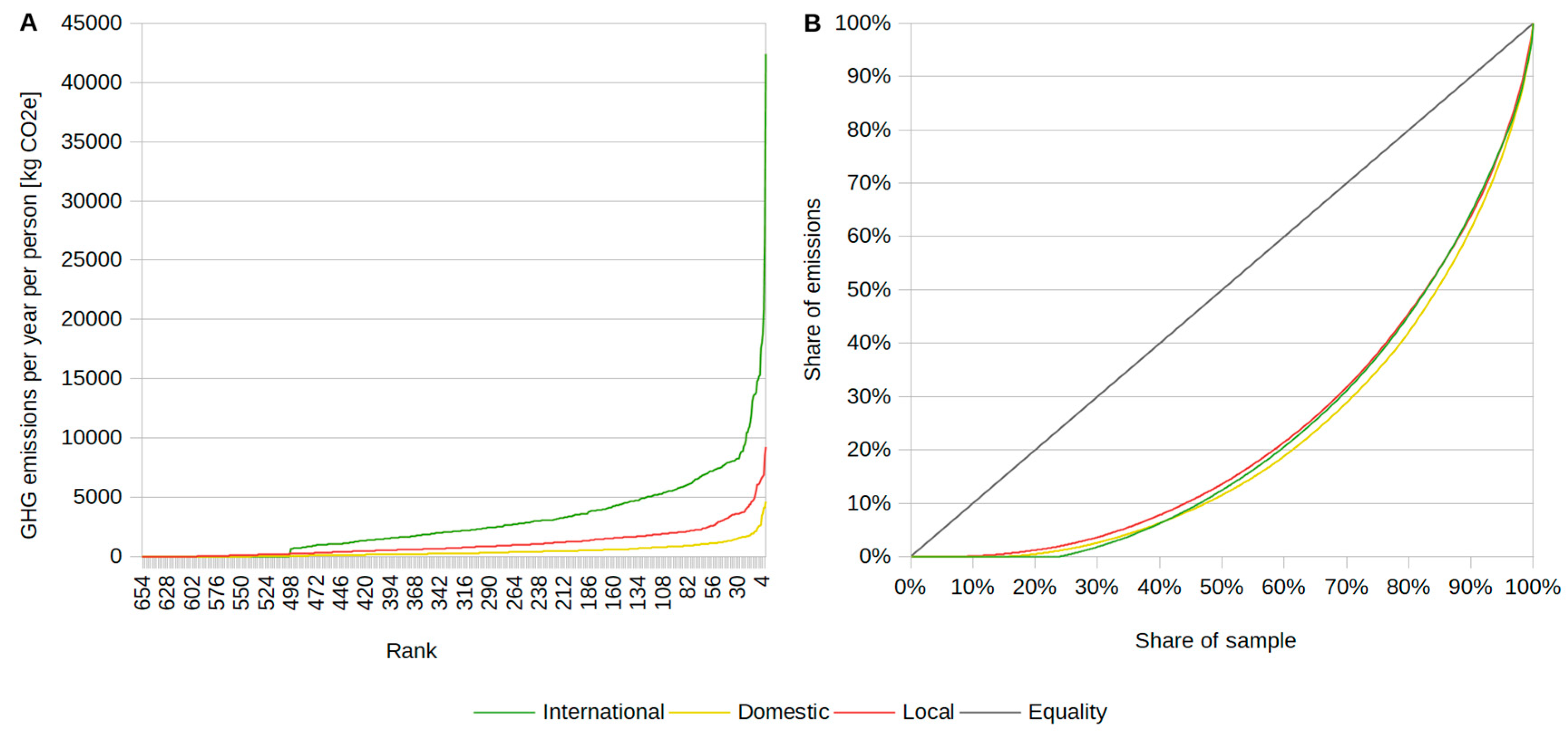
3.1.1. Unequal Distribution of Travel Emissions

The structure of travel emissions was highly unequal, as illustrated by the Lorenz curves in Figure 2b. The top 20% of emitters were found to generate 60% emissions in local travel, 58% emissions in domestic leisure travel, and 55% emissions in international leisure travel. The distributions followed the pattern detected by Brand and Preston [21] in the travel of UK residents, and as found often in patterns of consumption at various scales [66]. The curve of international travel emissions in the rank chart (Figure 2a) increases abruptly around 8 tCO2e per year per person. The participants above that point were the top 5% emitters: hypermobile individuals who make, on average, 7.7 trips abroad and generate about 22.5% of the emissions of the study participants.
About one-quarter of the respondents did not participate in international travel at all in the 12 months before the survey, which is a long enough period to interpret that they either travel internationally very little or not at all.
Importantly, the unequal distribution of the emissions from travel is only loosely related to income levels. The emissions generated by international travel of the highest income group are higher than those of other groups (Figure 3). However, among the top 5% emitters in international travel (n = 32, marked by a steep increase of the green line in Figure 2a and shown as outliers in Figure 3) there were members of all income groups: five of them belonged to the lowest income group (<290 k ISK (Icelandic króna, 1000 ISK = 7.9 EUR (Euro) as of 12 September 2017.) per CU) and seven belonged to the highest (>670 k ISK per CU). In the whole sample, the rank correlation between income per CU and emissions from international travel was weak but significant (ρ = –0.18, p < 0.001). The income elasticity of international travel emissions, calculated as a correlation between logs, was quite low and produced a Spearman’s rank correlation of 0.145 (p = 0.002, n = 465).

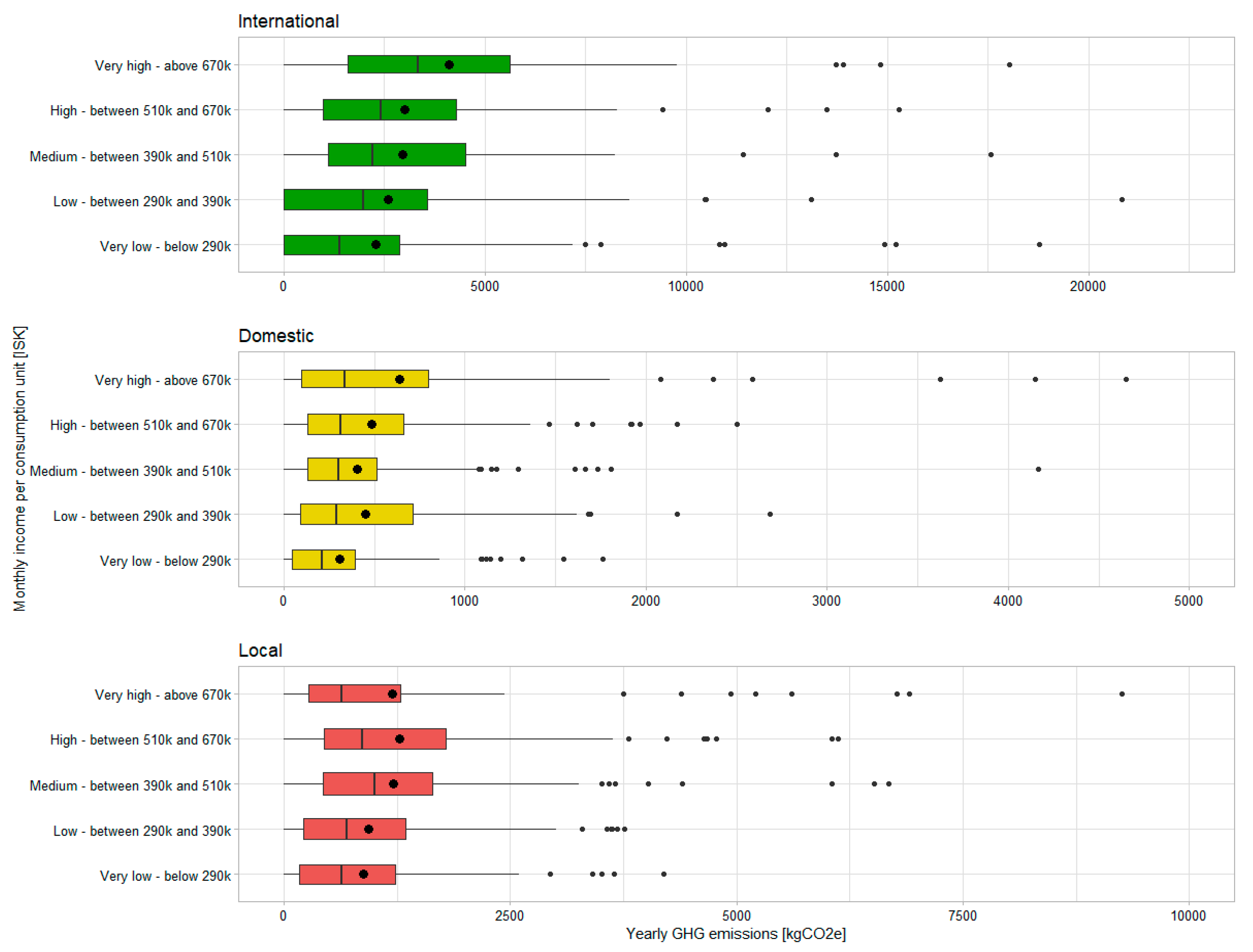
3.1.2. Characteristics of More and Less Mobile Groups Distribution of Travel Emissions

Following the findings presented in the previous section, the respondents were divided into four groups based on their overall GHG loads from leisure travel to analyze the characteristics of the more and less mobile people: Non-emitters, middle group, top 20% emitters, and top 5% emitters. As shown in Table 1, the different groups carried some distinct features. Compared to other groups, the non-emitters group was characterized by a somewhat lower share of people with graduate or postgraduate education (32%) and a lower percentage of people who speak four or more languages (8.4%). The non-emitters tend to live farther away from the city center than those who travel abroad. Relatively, many of them (17%) have no car in their household. Their incomes are somewhat lower than those of other groups, but the difference was not large. The top 20% and top 5% emitters differed from the other groups by having a higher proportion of people with graduate education (39% and 44%, respectively), a higher proportion of people who speak many languages (19% and 37.5%); in addition, these groups are more likely to live in the urban core of the region.

3.1.3. The Internal Structure of Travel Emissions

International leisure flights dominated the overall emissions of a travel-related carbon footprint of an average young adult in Reykjavik with an almost two-thirds share (66%) and an average of 2.96 tCO2e/y/p. Trips within the urban region only generated 24% of the overall GHG emissions, and leisure trips away from the city but within Iceland were yet a much lower 10% (Figure 4).
The dominance of international travel would be more pronounced if only emissions from fuel combustion were taken into account. The vast majority (92%) of emissions from flights results from fuel combustion, with a relatively small contribution (8%) by emissions embedded in aviation vehicles and other infrastructure. Local and domestic car travel are the second and the third contribution to the travel-related footprints, averaging at 1.08 and 0.45 tCO2e/y/p, respectively. A relatively large part of these emissions is embedded in vehicle production and road infrastructure: 32% in local travel and 42% in domestic travel. The difference is largely due to higher reported car occupancies in domestic leisure trips than on local trips. The figure suggests that efficiency gains in private cars, such as their electrification, have only a limited potential of decarbonization, especially when vehicle production remains as carbon-intensive as it is now (see, e.g., [55,67] for vehicle production GHG analyses).
Domestic flights have by far the highest carbon intensity at 0.311 kg CO2e/pkt, followed by domestic ferries (0.258 kg CO2e/pkt), but these travel modes were rarely chosen by study participants and did not importantly contribute to average travel carbon footprints.

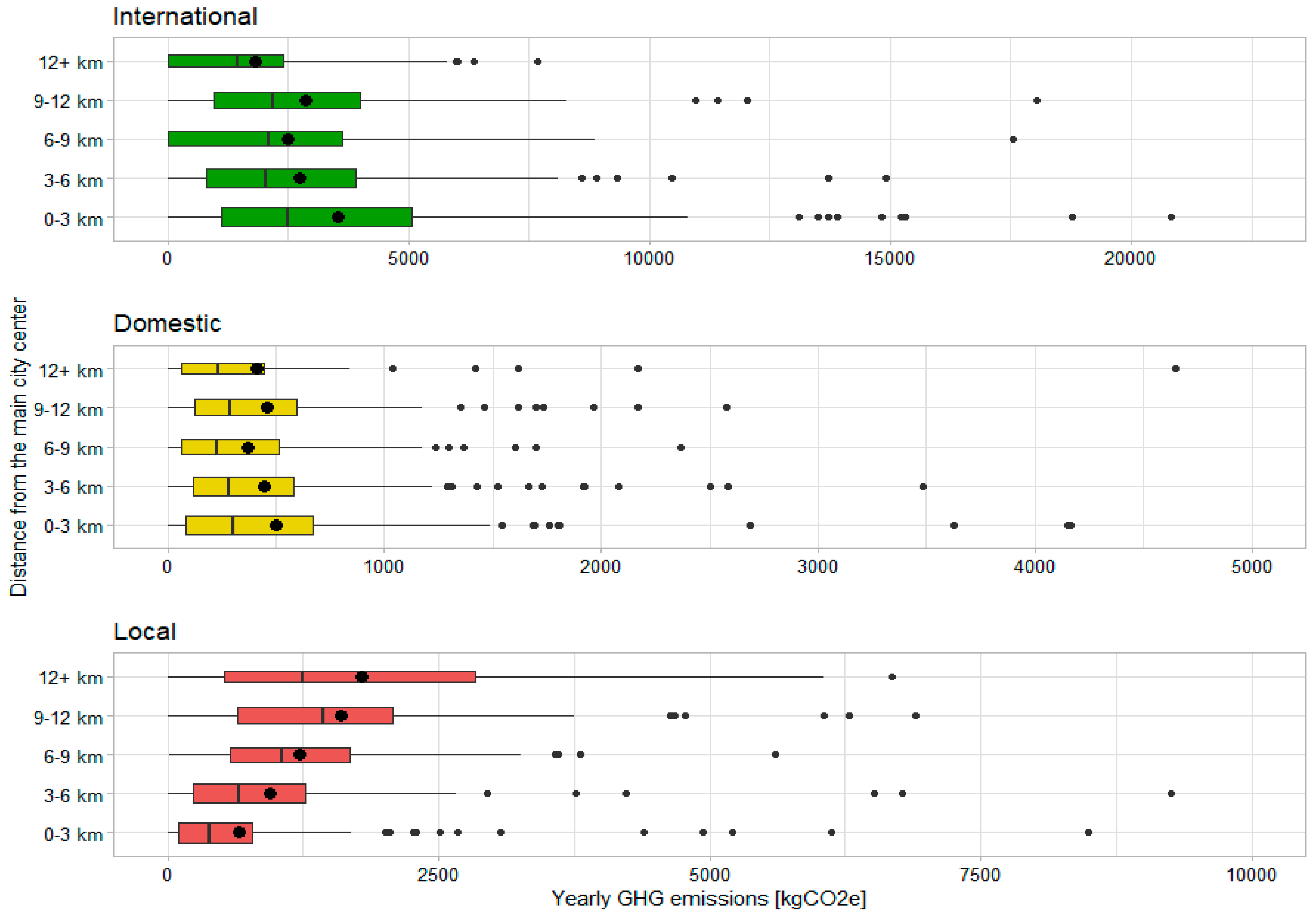
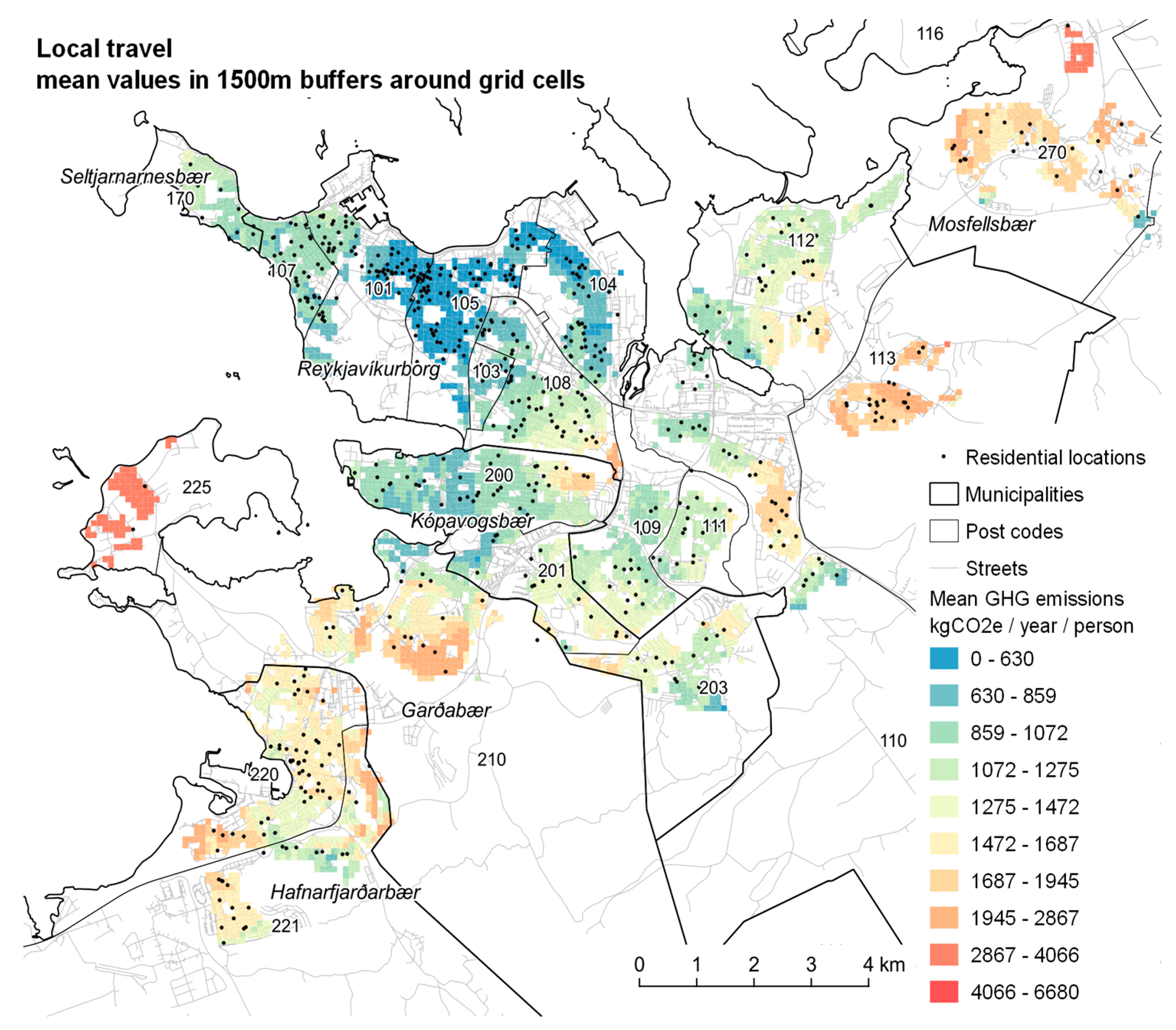
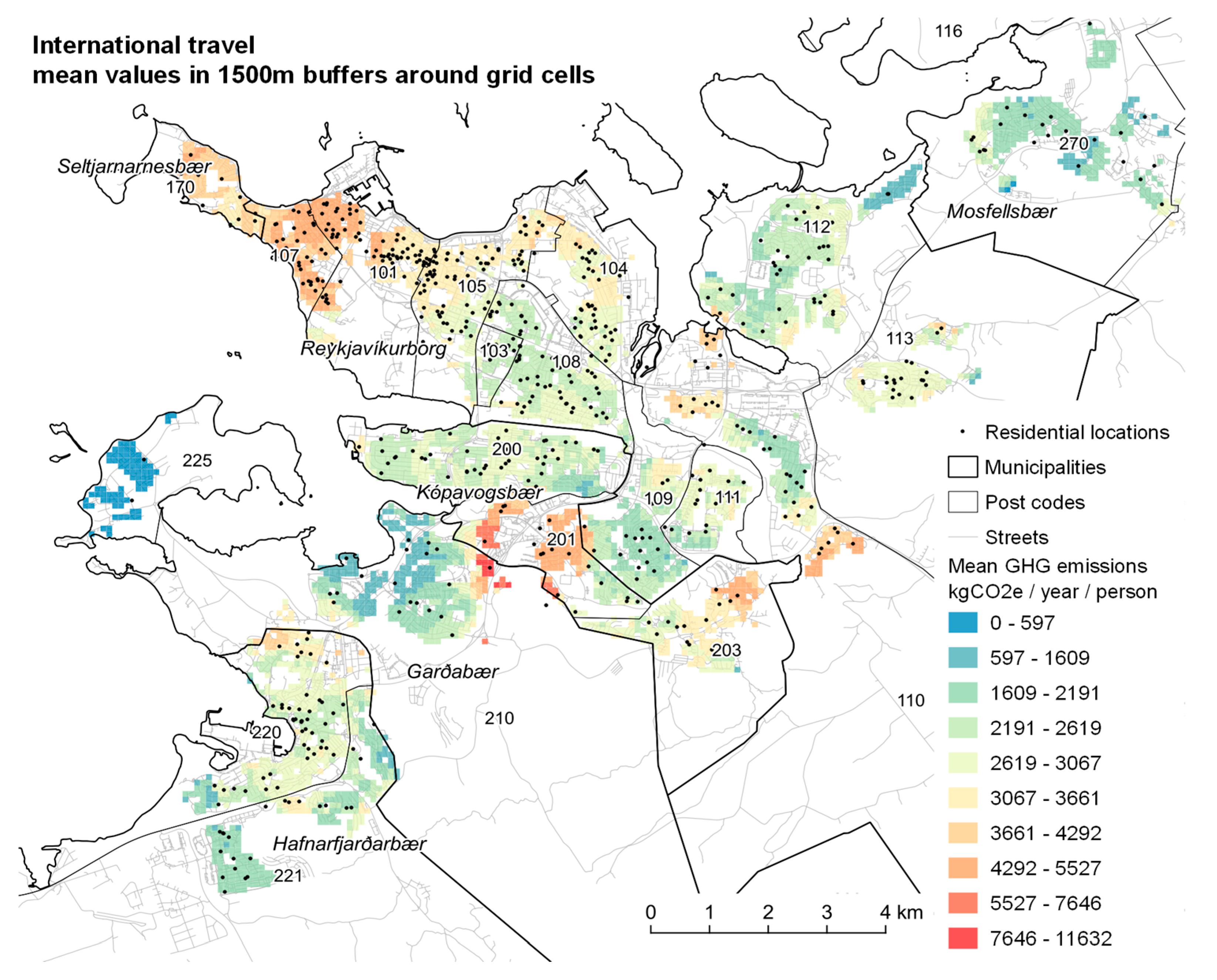
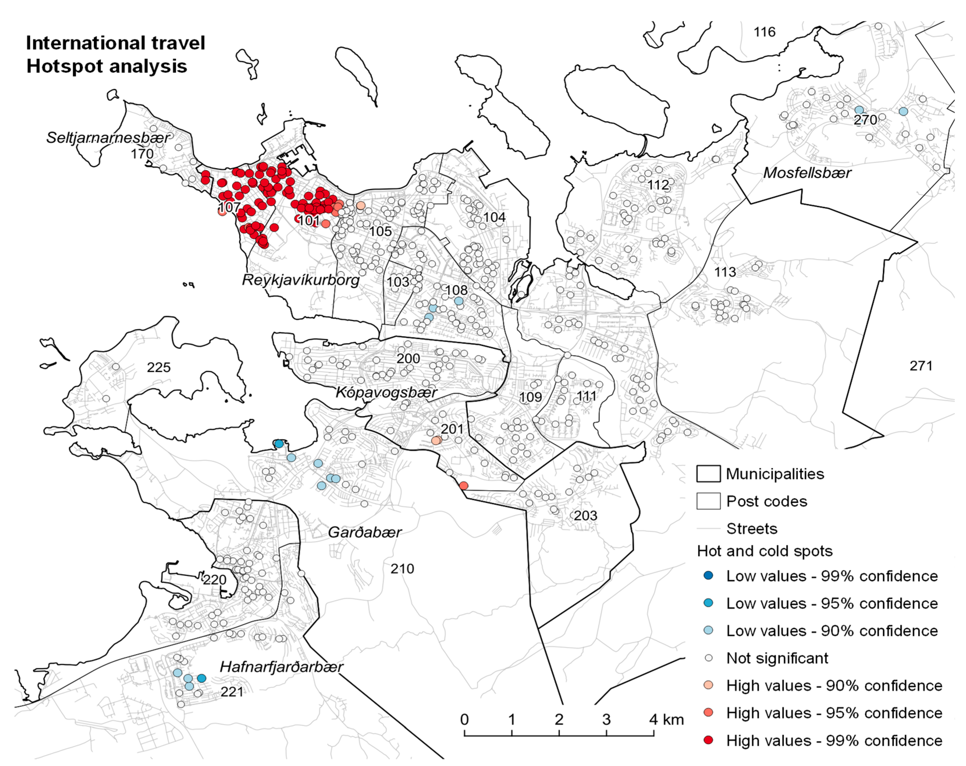
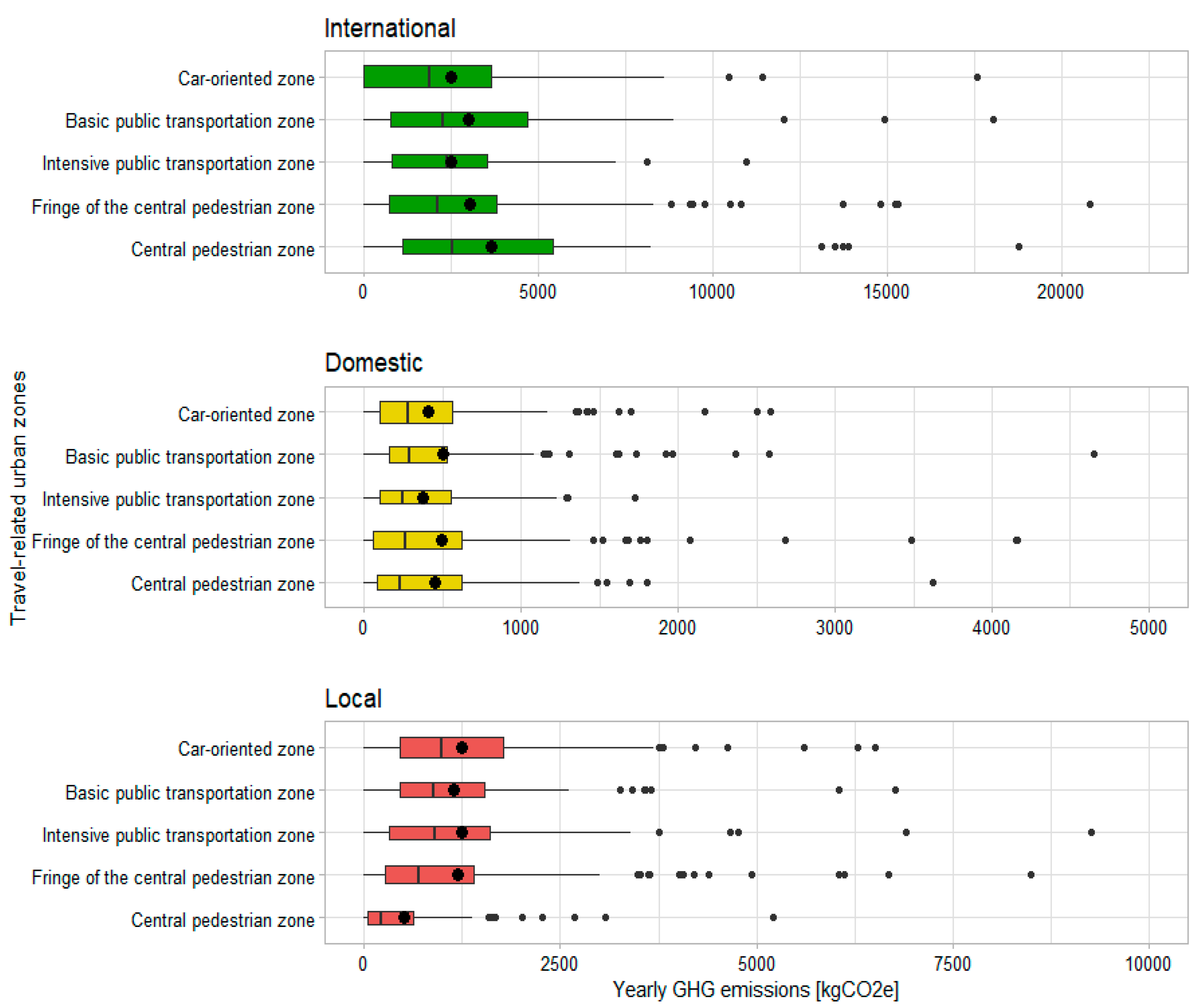
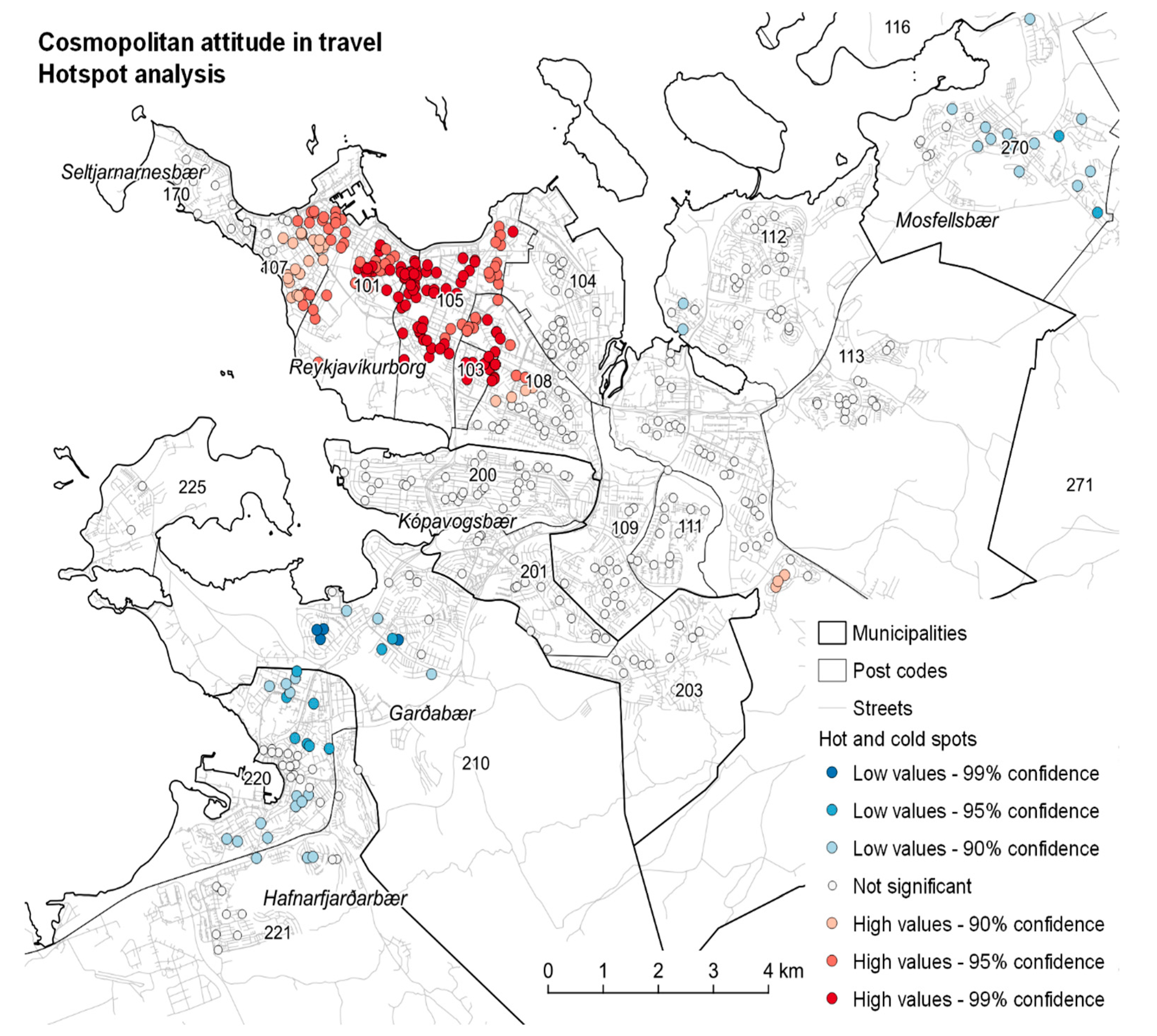
3.1.4. Geographical Distribution of Travel Emissions

The geographical analysis of the average per capita emissions revealed that emissions from local travel increase when moving away from the most central and pedestrian-oriented areas. Emissions from domestic travel did not appear related to the urban structure, and emissions from international travel increased towards the inner city locations (Figure 5). The pattern is similar to that found previously in Helsinki [17]. Importantly, emissions from long-distance travel were found to dominate the overall GHG loads from transport regardless of the distance to the city center or the urban zone, even though they were more pronounced in the inner-city areas. The correlation between emissions and the centrality of the location was steeper in the case of local travel than in the case of international travel, but the vast amount of emissions from aviation overshadows the mitigation gains resulting from the compactness of the urban form. The patterns were visible, even if less pronounced when travel-related urban zones were used to measure the urban structure (Figure A1).
There is a significant spatial association of GHG emission values from local travel with Moran’s I = 0.146, statistically significant at p < 0.001 level. The emission levels from other scopes of travel did not spatially cluster, according to Moran’s I statistic (Table A7).
The highest average emissions from local travel (above 2 tCO2e per year per person) were found to be concentrated in peripheral areas (e.g., postcodes 113, 270, and 210; Figure 6). The lowest average emissions from local travel (below 0.6 tCO2e) were found to be concentrated in the city center (postcodes 105, 104, and 101 in Reykjavík; Figure 6). The hotspot analysis (Figure 7) confirmed the central areas as clusters of high values and the suburban postcode 113 as a significant cluster of low values. In general, the emissions from local travel increase with increasing distance from the city center.
The highest average emissions from international travel (ca 4 tCO2e per year per person) are concentrated in the city center (postcodes 107 and 101; Figure 8), and one peripheral area (postcode 201; Figure 8). The hotspot map (Figure 9) shows that only the centrally located cluster of high emission levels is significantly different from the regional average.
The emissions from domestic travel did not show any significant spatial association and thus are not shown on the maps.

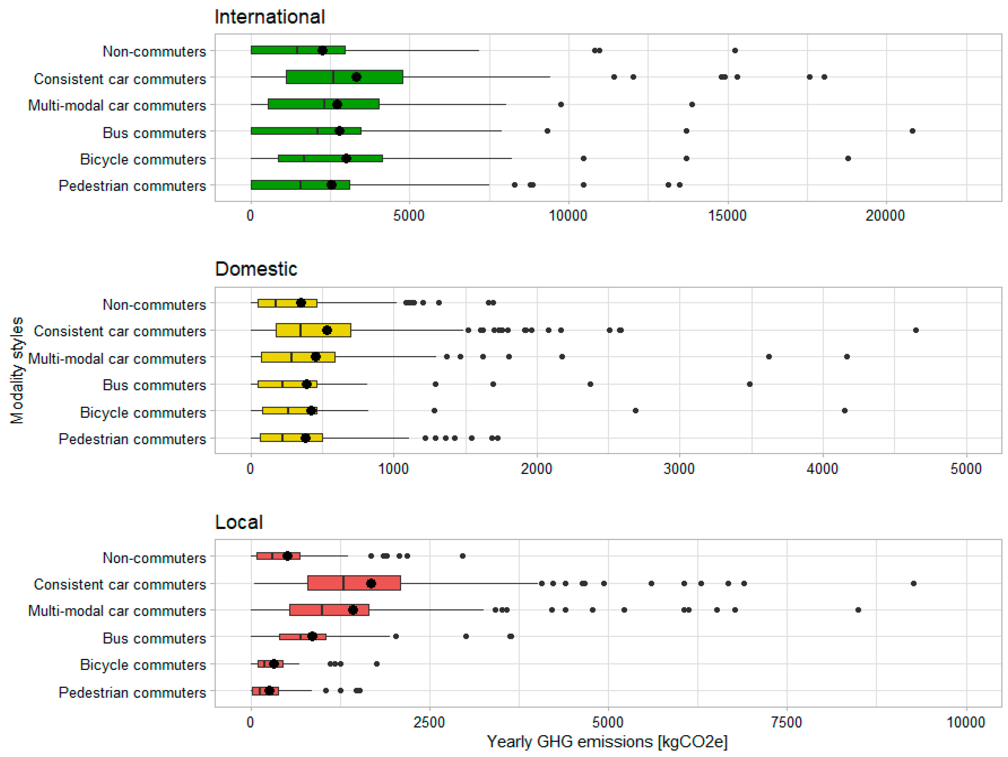
3.1.5. Travel Emissions and Modality Styles

The geographical patterns might seemingly indicate a kind of a trade-off between car use and private flights, as suggested earlier by Ottelin et al. [8,27]. However, the analysis of emissions of different modality styles showed that those who drive private cars daily and generate high emissions in local travel also generate high emissions from international travel. The group with the highest average emissions from international travel are the consistent car commuters (ca 3.5 tCO2e), followed by the bicycle commuters (ca 3.0 tCO2e), and the pedestrian commuters (ca 2.8 tCO2e) (Figure 10). This pattern appeared to be independent from a residential location. Compared to other groups, consistent car commuters have the highest levels of emissions from travel abroad in the central pedestrian zone (4.7 tCO2e/y/p, n = 17), its fringe (3.7 tCO2e/y/p, n = 43) and in the car-oriented zone (3.6 tCO2e/y/p, n = 97; Table A8). The pattern is not dependent on income levels either.
Car ownership was not found to systematically related to international travel either. Those who own more than two cars in a household appear to generate the lowest level of emissions. Those who own two cars generate the highest emissions, which might be related to high incomes in this group. The differences between the other groups are negligible (Figure 11). Furthermore, the relationship between car ownership and international travel does not show any visible geographic pattern and does not appear to be dependent on income levels.
Interestingly, the top 5% mobile group has a higher percentage of inner-city residents, pedestrian commuters, and car-less households than the less mobile groups (Table 1), so the effect of substituting city driving with flights abroad might be limited to the hypermobile people.

3.1.6. Travel-Related Emissions and Climate Change Awareness

There was a relatively small number of people in our sample (13%–20%, depending on the item), who disagreed with or were unsure about the climate change-related statements that are in line with academic consensus. These people have lower average levels of emissions from international travel than those who agree with the statements (Figure 12). However, the median was similar across the groups, and the averages in the groups with high climate change awareness were higher due the presence of the highly mobile individuals (shown as outliers in Figure 12). As shown in Table 1, the highly mobile people tend to speak more languages and have a higher level of education than other groups, which suggests that the correlation between climate change awareness and high emissions from travel abroad is related to cultural capital.
Those who disagreed or were unsure about the statements were shown to be somewhat less likely to speak multiple languages or have a university degree than other groups, but they were not found to differ in terms of income levels (Table A9).

3.2. Multivariate Analysis

The regression analysis provided an insight into which characteristics correlated with participating in certain travel behaviors and with the level of emissions associated with these behaviors when other variables were controlled.

International Travel Emissions

Single people and families with children are less likely to travel abroad than couples (Table 2). Having a low monthly income level also decreases the likelihood of taking at least one leisure trip abroad in the previous year. A cosmopolitan attitude in travel (Factor 3) is the strongest predictor of participation in travel. It also appears to be clustered geographically, with high values concentrated in the city center (Figure A2). It thus appears that the geographical trends described in Section 3.1.4 could be largely explained by the spatial clustering of cosmopolitan and travel-positive attitudes in the city center (see also [18]). Climate change awareness (Factor 2) significantly, even if weakly, was found to increase the likelihood of traveling abroad, even when the education level was controlled in the model.
GHG emissions associated with domestic travel are the most strongly and positively associated with having access to a summer house and having preferences towards spending leisure time in natural vs. urban environments (Table 3). Moreover, women are more likely to participate in domestic leisure travel than men, and those who have a car in the household are more likely to engage in domestic leisure travel than those who do not. We found no significant association between emissions from domestic leisure travel and the urban form (e.g., neighborhood greenness, distance to the city center, or access to a private yard) or household income. When comparing mean trip frequencies and the level of emissions between different groups, those living in apartment buildings and without a private yard were found to travel more often and for longer distances domestically than other groups (Table A6). Therefore, these aspects may potentially play some role in motivating domestic travel behaviors, even if this was not shown to be significant in the models.
The amount of emissions from local travel were found to be positively associated with increasing distance to the city center, a medium or high weekly workload, and having a graduate or postgraduate degree (Table 4). Pro-car attitude is a strong predictor of the emissions from local travel, followed by preferences towards residing in suburban vs. urban neighborhoods. Preferences for shared housing and transport are negatively associated with emissions from local travel. Interestingly, having more cosmopolitan attitudes towards travel is associated with higher emissions from local travel.
We performed a residual analysis and collinearity diagnostics on all linear models. The residuals showed no signs of heteroskedasticity in the Ln models, as their distribution was symmetrical, without patterns, and clustered towards the middle of the plots. The residual plots of the untransformed models were highly skewed, which was expected due to the character of the outcome variable. We thus did not report the significance levels of these models. In all cases, Variance Inflation Factors (VIF) were below five and tolerant above 0.2, indicating that multicollinearity was not strong.

4. Discussion and Conclusions

This study aimed at quantifying the structure and geographical distribution of GHG emissions from the local, domestic, and long-distance travel of the young adults of Reykjavik. Furthermore, the factors influencing this structure were studied, with a particular focus on how the residential location within the urban region and the awareness of climate change influence emissions from travel, as well as whether we could identify other factors.
We found that the overall travel-related GHG emissions were dominated by those resulting from long-distance flights, regardless of residential location, modality style, or income level, except for those residing furthest away from the city center (12+ km). Moreover, the level of GHG emissions from long-distance travel alone reached three tons of CO2e/y per capita, which is more than 50% of the currently available global per capita carbon budget to follow the Intergovernmental Panel on Climate Change (IPCC) pathway to 1.5-degree warming [1]. These findings are in line with those of recent studies of Helsinki in Finland [17,42], although we found slightly lower overall emissions and higher long-distance travel-related emissions in Reykjavik than in Helsinki. For the consistent car-commuters, the overall GHGs from the transport were found to exceed 5.5 t CO2e/y per capita and to transgress the whole current per capita carbon budget without emissions from any other consumption taken into account.
We found the emissions from international leisure travel to increase towards the city center, reaching nearly five tons in the city center and its surroundings, approximately the current annual average global per capita emissions [1]. The geographical trend is in line with previous research [17,18,23,31,68]. When socio-psychological factors, such as cosmopolitan attitudes, were controlled in regression models, distance to the center lost its significance. This result supports the hypothesis of cosmopolitan orientation as a reason behind the elevated levels of international travel of inner-city dwellers in Nordic cities [18,23,68]. The level of language skills was another important predictor, which, together with the impact of education level known from previous research, suggests that cultural capital may be another driver of the aggregate geographical patterns. Even though we did not directly measure properties of participants’ social networks, the results point to the importance of the globalization of lifestyles in motivating the international travel of the educated urbanites, as suggested elsewhere [13,20]. Even though income remains an important predictor of emissions from international travel, in line with previous studies (e.g., [20]), its predictive power in our sample was relatively low. This result suggests that in affluent societies, such as that in Reykjavik, ticket prices are no longer a strong hindering factor in long-distance travel decisions.
Domestic travel was found to generate the lowest share of total travel-related emissions, and it did not significantly correlate with the residential location and the urban form around it (i.e., population density, distance to the city center, neighborhood greenness or access to a private yard). Our results suggest that domestic travel patterns do not play any strong role in the first contradiction discussed in the introduction. Furthermore, we did not find any evidence to support the compensation hypothesis, which has been suggested previously as a potential factor explaining the increase in the amount of long-distance travel towards the city centers (e.g., [69]). Access to a summer house and preferences towards spending leisure time in natural vs. urban environments were found to be significant predictors of the emissions from domestic travel. It thus appears that domestic travel is motivated more by personal preferences and access to facilities rather than by the urban structure itself.
Results related to local travel emphasize a strong geographical trend of increased car use and emission levels farther away from the city center and in car-oriented areas, which is in line with previous research conducted in the Nordic countries and elsewhere (e.g., [7,70,71]). Of multiple urban form variables tested in models, distance to the main city center was the strongest predictor of emissions and remained significant after controlling for sociodemographic variables and attitudes, which supports the results by Næss [7]. Our results also emphasize the importance of attitudes and preferences related to travel modes and residential location in predicting the level of emissions from local travel, but they do not undermine the role of the urban form, which has been shown to have a causal effect on travel behavior [11,12].
We also detected a highly unequal distribution with all the three types—local, domestic, and international—of travel, meaning that the high average emissions are a result not only of a high level of mobility through the majority of the population but also the presence of the highly mobile minority. This result followed the pattern detected, e.g., in the UK before [19,21]. At the same time, a relatively large fraction of the sample did not seem to participate in long-distance travel at all. We consider this a deliberate choice or a sign of disinterest in travel, as the question about trips referred to 12 months before the survey, which should be a long-enough time-span to capture some trips for those who actively travel. Later in this section, we discuss the policy implications related to this issue.
Similarly to Alcock et al. [19] and Árnadóttir et al. [42], we found pro-environmental attitudes and climate change awareness to predict more flights and a higher GHG load, not less. Defining this as a causal relationship between these two variables would be incorrect, though. The respondents concerned for the environment share several qualities related to participation in and frequency of long-distance travel, such as better language skills and higher education. Furthermore, we cannot trace the origin of their concern, particularly whether it relates to traveling and seeing the world or not. We also observed an attitude-behavior gap in local and domestic travel; climate change awareness and pro-environmental attitudes either had no significant effect or a positive association with emissions and participation. While positive associations are difficult to explain, the lack of action from concerned respondents to minimize their car use could stem from an unwillingness to drastically change lifestyles due to a habit or routine, comfort and convenience, or a perceived lack of efficient and cheap public transportation [72].

4.1. Strengths and Limitations

Among the strengths of this study is its use of a broad-scope LCA-based GHG factors in the assessment, including the direct emissions from fuel combustion, fuel production, and transport, vehicle manufacturing, and transport infrastructure production following the suggestion of Chester and Horvath [49]. Of our GHG load estimates, the indirect components explain 32%–42% of shares in local and domestic travel, confirming the importance of including them. We also used the emission coefficients for air travel that take a higher radiative forcing effect of emissions in the high atmosphere into account, thus more realistically estimating the global warming potential [56]. It is also one of the few studies that include both short- and long-distance travel, allowing us to compare the climate impacts and different factors of these two and thus emphasize that various travel scopes should be studied in combination and not separately.
The limitations of this study included a relatively small sample that did not allow for the conduction robust analyses of small groups to study more complex relationships and interactions. Another limitation was the focus on young adults, which reduced the ability to generalize the results to the whole population of the study area. Broader generalizations were also limited by the somewhat exceptional characteristics of Reykjavik as a study area, mostly due to its location on an island and thus having fewer alternatives to air travel when going abroad. Moreover, the climate in Reykjavik is rainy and cold in global terms, which might encourage more leisure trips away. Studying this potential explanation would, however, require detailed information about the stated and potentially latent reasons for leaving, which the survey utilized in this study do not provide. Still, as stated in the introduction, the unique characteristics of Reykjavik also make it an interesting case to study, and the results of this study provide a benchmark or a point of comparison to future studies in other locations.

4.2. Further Studies

There is a need for more transportation-related studies that focus on the climate impacts of trips at different geographical scopes (i.e., local, regional, domestic, and international). Ideally, studies should report emissions generated from an LCA, along with those from fuel combustion and energy production. Other studies should replicate the results in other wealthy regions, due to the high level of travel emissions there, but also in regions with a strong upward trend in aviation and tourism, such as China, Latin America, Central, and Eastern Europe. Comparisons between multiple cities or regions with varying levels of access to international airports, different socio-economic structures, and different urban forms would also contribute well to the literature.
Notably, the regression models that predicted emissions from local travel had markedly a higher predictive power than those on domestic and international travel. Long-distance travel models may not include all relevant and measurable variables and thus suffer from misspecification. Future studies should include more variables, such as social network characteristics and mobility biographies [73,74,75], and a more refined measurement of socio-psychological characteristics. More qualitative and mixed-methods studies and conceptual work are needed to identify other potentially relevant factors. Longitudinal data would help to track changes in time and their factors, especially in the light of high growth in aviation and tourism, and changing debates about climate change and the climate impacts of travel. Furthermore, larger samples from quantitative surveys would help in creating stronger and more sophisticated regression models and small-group analyses.
Other possible dimensions of the topic that have not been studied well enough include the characteristics of visited destinations and motivations to visit places, including links to well-being. These and other topics can and should be studied with qualitative and mixed methods, which would greatly improve the understanding of the causal links behind the aggregate patterns and motivations of individuals. Among the issues that are highly relevant to policy-making and could be well studied with a mixed-methods approach are sensitivity to the changing cost of flights, links between environmental and climate change concerns and mitigating behaviors, the perceived difficulty of behavior changes, the role of social norms, and the role of cosmopolitan attitudes and globalized lifestyles in motivating travel.

4.3. Policy Outlook

In this paper, we have shown how flights can dominate the emissions from transport in an affluent location despite high levels of emissions resulting from ground transport. We have also shown how the emissions from flights tend to rise along with reduced ground transport emissions. This situation urges discussion on effective policies to radically reduce the emissions from transport overall, not just from one mode—with potentially consequential reverse impact on the others. Furthermore, it seems to be largely different policies and policy-levels which affect local ground transport emissions, domestic ground transport emissions, and long-distance travel emissions.
The prevailing global policy-orientation is to densify urban areas to reduce emissions from private driving. Previous studies have found this as an effective policy [6,7]. We also found significant reductions in local transport emissions in Reykjavik, although in Reykjavik, even the most centrally located dwellers typically possess cars and generate a relatively high amount of emissions from car travel. Our results emphasize that densification should focus on densifying areas close to the main city center and main concentrations of jobs, not necessarily local urban design characteristics [12].
Planning policies related to urban density have recently been criticized as insufficient for GHG mitigation [9,13]. One suggested mechanism that hinders densification from leading to GHG mitigation is the rebound effect following reduced driving and car possession, particularly as increased flight activity [8,27]. In this study, we found little evidence of such a rebound. It may well be in Reykjavik that almost all the residents are affluent enough to fly and possess vehicles if they choose to. Reykjavik is also a very strongly car-oriented city by its design and the mindset of the residents, and households that redirect their spending from car ownership and use to private flights might be too few to influence aggregate patterns.
We also have not found any plausible causal link between urban density or central location and the higher amount of international travel. The apparent correlation between urbanity and travel abroad most likely results from tendencies among people of certain socio-psychological characteristics (e.g., cosmopolitan attitudes and high cultural capital) to locate in central urban areas. Therefore, the results of this study do not challenge the current densification policies (see [31]), but instead, they suggest that land use and transportation planning measures should accompany policies aimed at reducing emissions from long-distance travel.
Policies directly related to international aviation are necessary if total transport emissions are to be reduced. The aviation industry mostly relies on efficiency gains [76] and offsetting [77]. However, as shown by Peeters et al. [78], the efficiency gains are outpaced by growth in trip numbers and distances, and technological solutions are ineffective in reducing total emissions from aviation. Indeed, the most promising emerging technology of all-electric aircraft is unlikely to be operational within the next 20 or 30 years and require significant improvements in battery technology [79,80]. Other policies are necessary, ideally such that would halt or reverse the growth in demand for flights.
Participants of the “Stay Grounded: Degrowth of Aviation" conference 12–14 of July 2019, Barcelona, Spain recently discussed a set of such policies (see [81] for short summaries). One of the suggested policy measures, which might prove efficient in the context of Reykjavik, was a progressive aviation tax in which ticket prices increase along with the increasing number of flights per year. Such a policy is under the power of different decision-makers than urban densification, but the two together could lead to efficient overall GHG mitigation from transport. A taxation on kerosene used in aviation and value-added tax on flight tickets are other, more conventional, suggestions, although they have been criticized for hitting the poorer part of the population the hardest. Limits and bans have also been suggested, although they are considered a feasible option on short-haul flights only.
Overall, tourism is a sector calling for more attention in the context of climate change mitigation. The global emissions are growing fast, driven particularly by flights [82] and, per trip, can be of a magnitude similar to average annual carbon footprints in relatively affluent countries [83]. It has also been recognized that such trips may fall outside the sphere where environmentally conscious consumption decisions are made [19,42]. While the above-described aviation taxes would cover tourism, additional measures might be needed. One measure, implemented fully or partially in several locations, is a tourist tax on services (and goods) tourists frequently use [81,84], such as hotels (in use around the world), restaurants, car rentals, tourist attractions tickets and so on. The effect of these taxes is not only limited to the minor share of the overall tourism GHGs for which these services are responsible, but they also affect the “getting there” part, which typically causes the main GHG load [58,82] by making trips more expensive overall. The other way round, GHGs could be mitigated without an intention to cut down travel activity by making alternative travel modes, particularly ground transport, more competitive in comparison to flying and by supporting the development and the rapid market penetration of low-carbon technologies [81].
Though our results suggest that high climate change awareness and a pro-environmental attitude do not lead to lower travel emissions, this could be changing. Our data were collected before the increased discourse on flygskam (English: flight shame) [84,85], which became more apparent in Iceland at the beginning of 2019. Previous research has suggested that targeting people’s social identity and a need to conform could be effective in changing behavior [35], so if there exists a social norm to travel extensively, the discourse on flygskam presents an opportunity for changing that norm and in turn mitigating emissions from flying. There is also the potential of the phenomenon changing into a kind of a lifestyle movement whose members not only modify their behaviors and lifestyles but also actively engage in social and political change [86]. As a lack of action by governments is a barrier for taking individual climate action [72], a changed discourse presents the potential for more support for policies directed at mitigating long-distance travel emissions, which could consequently reduce that barrier.
Based on the findings of this paper and the discussion above, it seems obvious that a more active role of cities and national governments of wealthy countries in shaping the consumption patterns of their residents, including aviation, is needed. They should also recognize the risks of rebounds related to long-distance travel when pushing densification policies forward. Regarding the case of Reykjavik, even though we didn’t recognize strong rebounds, there are mechanisms that might lead to increased long-distance traveling if the current densification plan manages to reduce the currently extremely high car-dependency. For example, people travel when they have holidays, and, without cars, they are more likely to fly. We have yet to see how social phenomena, such as flygskam, affect demand in aviation, and whether globalization continues and induces the demand. Local, national, and global policies can play an important role in shaping the future in this regard.

Author Contributions

Conceptualization, M.C. and J.H.; methodology, M.C.; formal analysis, M.C. and Á.Á.; data curation, M.C. and J.H.; writing—original draft preparation, M.C.; writing—review and editing, M.C., J.H. and Á.Á.; visualization, M.C. and J.H.; supervision, M.C. and J.H.; project administration, J.H.; funding acquisition, M.C. and J.H.

Funding

This research was funded by The Icelandic Road Administration Research Fund (Rannsóknasjóðs Vegagerðarinnar), The National Planning Agency Research and Development Fund (Skipulagstofnun Rannsóknar- og þróunarsjóður), and The University of Iceland Research Fund (Rannsóknasjóður Háskóla Íslands).

Conflicts of Interest

The authors declare no conflict of interest. The funders had no role in the design of the study; in the collection, analyses, or interpretation of data; in the writing of the manuscript, or in the decision to publish the results.

Appendix A. Methods

Appendix A.1. Trip Distances and Frequencies

We calculated distances to international and domestic destinations visited by plane and international locations visited by ferries as geodesic shortest distances between home and the destination in a Spatialite database using The World Geodetic System 1984 (WGS84) coordinate system to take the curvature of the Earth into account. We treated every regional and international destination as a two-way trip. We corrected the distance estimation by multiplying by 1.2 per interchange to account for the deviations from the shortest distances that result from the interchanges.
Distances to international destinations not originating in Iceland and visited by car, bus, or train, were calculated as geodesic shortest distances and multiplied by a “detour factor” of 1.417 to account for the deviations from the shortest distances that result from the street and rail network layouts.
Distances to domestic destinations visited by car, bus or ferry were calculated along the road network data obtained from the IS 50V topographic map of Iceland, as well as the ferry network data obtained from EuroGlobalMap and OpenStreetMap and checked with ferry operators’ websites. The distances between home locations and destinations were then calculated using the Route tool in the Network Analyst toolbox in ArcMap 10.
We calculated distances to local destinations along the street network data obtained from OpenStreetMap for walking and cycling, and we used the i50v topographic map for car and bus. The distances between home locations and destinations were then calculated using the Route tool in the Network Analyst toolbox in ArcMap 10.
The frequencies of local trips were measured in categories related to weekly or monthly periods (e.g., “five to seven times a week” or “once or twice a month”) and numerically coded to estimate the number of trips made during previous 12 months. The reported number of trips in regional and international travel was also numerically coded and used to estimate the number of trips in 12 months. The yearly distance traveled to each of the marked destinations was then estimated by multiplying distances and frequencies.

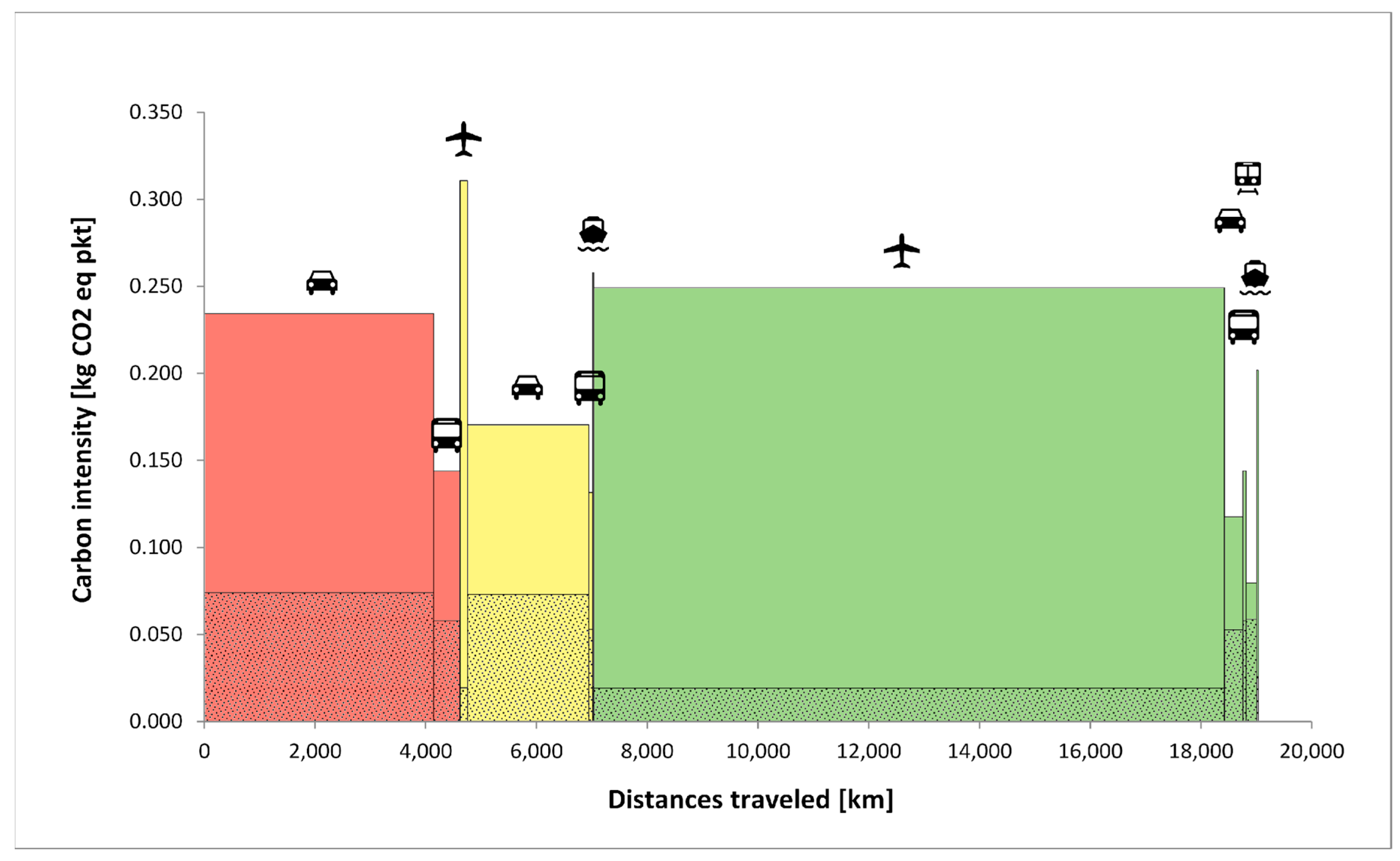
Appendix A.2. Emissions Estimation with LCA

Direct emissions (i.e., fuel combustion) for private cars were based on the fuel efficiencies and occupancy rates reported by the survey respondents. The fuel efficiency was asked with a five-category question with options from below 4 L per 100 km (L/100 km) up to over 10 L/100 km with two-liter intervals and separate options for electric vehicles. For those who did not answer the question on fuel efficiency, the average of 7.6 L/100 km was assumed. For the trips without data on car occupancy, the average occupancy rates of 1.3 for local trips and 1.9 for all other trips were assumed, following the LIPASTO database produced by the VTT Technical Research Centre of Finland Ltd. [87]. No occupancy data for Iceland were available. The estimated fuel consumption was turned into GHG emissions according to a GHG intensity of 2.36 kg CO2e/liter [88].
The direct combustion emissions of buses were taken from the LIPASTO database [87] following the average occupancy rate for natural gas buses in Finland. No Iceland-specific information was available.
The direct emissions for passenger airplanes were calculated with intensities taken from Aamaas et al. [15]. Following the resolution of the source, flights were split into short (<800 km) and long (>800 km) haul. The intensities include the short-lived climate forcers (SLCFs).
All the indirect emissions coefficients were drawn from Chester and Horvath [49]. The numbers include indirect emissions with a broad scope including fuel and vehicle production and maintenance, as well as also roadways, tracks, stations, runways, and other infrastructure. In Table X below, the GHG intensities for the fuel production component and the rest of the indirect emissions are separated.
Table A1. GHG emission coefficients per travel mode in CO2e kilogram equivalents per person kilometer traveled [kg/PKT].
Travel ScopeTravel ModeExplanation and SourcesDirect Emissions: CombustionIndirect EmissionsTotal Emissions
Fuel ProductionLife-Cycle
LocalCarReported fuel efficiency (liters per km, survey data) times 2.36 kg CO2e/liter [88], divided by 1.3 car occupancy [87]. Indirect emissions for San Francisco Muni [49].0.138 (average)0.0260.0740.238
BusNatural gas bus, the average occupancy rate in local traffic, 18/50 passengers [87].0.0690.0310.0500.150
Domestic and internationalPlane <800 kmLLGHGs and SLCFs included [15], indirect emissions for a midsize aircraft [49].0.300Included in combustion factor0.0200.320
Plane >800 km0.240Included in combustion factor0.0200.260
FerryHelsinki-Stockholm, average occupancy [87], indirect emissions for a midsize aircraft [49].0.2230.0150.0200.258
BusDiesel bus, average occupancy rate on long distance trips, 12/50 passengers [87].0.0490.0370.0580.144
TrainPendolino and intercity trains, average occupancy [87]. Indirect emissions for an SFBA Caltrain [49].0.022Included in combustion factor0.0620.084

Appendix A.3. Modality Styles

Table A2. The structure of travel modes in local travel (i.e., within the Reykjavik Capital Region) of the modality styles members.
Non-CommutingCommuting
Cluster CarBusFootBicycleCarBusFootBicycle
Bus commuters6010%82%4%5%37%22%36%5%
Consistent car commuters25891%3%3%3%88%1%9%2%
Non-commuters101----63%4%28%5%
Multi-modal car commuters14888%7%3%2%41%1%52%6%
Pedestrian commuters906%1%89%3%34%4%58%4%
Bicycle commuters6011%4%6%78%34%2%30%34%
Sample71762%11%16%10%60%4%30%6%

Appendix A.4. Urban Form Measures

The classification of the Reykjavik Capital Region into travel-related urban zones was based on the theory of three urban fabrics: a walking city, a transit city, and car city, as proposed by Newman et al. [62] and followed a similar classification performed in Helsinki and Stockholm described by Söderström et al. [63]. The definitions and calculations used in developing the urban zones for the Capital Region are presented in Table A3 below.
Table A3. The criteria used to delineate the travel-related urban zones structure of travel modes in local travel (i.e., within the Reykjavik Capital Region) of the modality styles members.
Zone NameDefinitionGIS Calculations
The central pedestrian zoneDensely built and populated, located within a walkable distance from the main commercial center (up to 1500 m), contains a high number and diversity of jobs and services, and has good access to public transport.Assigned to the cells within the contiguous area within 1500 m network distance from the main commercial center.
The fringe of the central pedestrian zoneDensely built and populated, located within a bikeable distance from the main commercial center (up to 3000 m) from the main commercial center, contains a high number and diversity of jobs and services, and has good access to public transport.Assigned to the cells within the contiguous area between 1500 and 3000 m distance from the main commercial center.
Intensive public transportation zoneThe area in which the public transport frequency is at least 10 departures per hour and walking distance to a bus stop is less than 5 min (332 m)Assigned to the cells not included in the above zones and having a bus stop with at least 10 departures per hour within a 5 min walk (332 m street network distance).
Basic public transportation zoneThe area in which the public transport frequency is at least 4 departures per hour and walking distance to a bus stop is less than 5 min (332 m)Assigned to the cells not included in the above zones and having a bus stop with at least 4 departures per hour within a 5 min walk (332 m street network distance).
Car-oriented zoneThe area in which the public transport frequency is less than 4 departures per hour or there is no bus stop within walking distance of 5 min (332 m)Assigned to the remaining cells, not included in the above zones.
We calculated the distance to the city center as the shortest driving route between each residential location and the point chosen to represent the center. The point was located at the corner of Laugavegur, Bankastræti, and Skólavörðustígur. The driving distances were determined with the Route algorithm in Network Analyst toolset in ArcGIS 10.5. The street network was based on the roads layer (samgöngur) from the i50v topographic map. The variable was calculated in kilometers.
Neighborhood greenness was calculated as a mean value of the normalized difference vegetation index (NDVI) calculated in 1 km straight-line buffers around each residential location. The index was calculated with Landsat 8 imagery downloaded from Earth Observing System’s (EOS) Land Viewer. The image was taken on 30th July 2016 with a 30 m spatial resolution. The index values were calculated in Raster Calculator in QGIS using the general formula: NDVI = (near-infrared channel − red channel)/(near-infrared channel + red channel). The specific formula for Landsat 8 is NDVI = (Band 5 − Band 4)/(Band 5 + Band 4). The mean values of the index in each buffer were then calculated using the “Raster statistics for polygons” tool in SAGA GIS.
Access to public transportation was based on the distance to bus stops and the average frequency of departures from the stops. The bus stops were divided into three classes: stops that have at least 10 departures per hour on average (waiting time about six minutes), stops that have at least four departures per hour on average (waiting time about 15 min) but less than 10 departures, and stops that have less than four departures per hour on average. Then, areas located within walking distance to the stops of each category were delineated using the Service Area tool in Network Analyst in ArcGIS 10.5. The threshold distance was 332 m, which roughly represented a distance that can be covered in five minutes by an average person. Then, the residential areas were assigned to four zones with access to bus stops of varying departure frequency.

Appendix A.5. Factor Analysis

Table A4. Rotated factor loadings retained in the four-factor solution. Answers to statements on page 11/14: Please state how much you agree or disagree with statements below (1 = strongly disagree, 3 = neither agree nor disagree, 5 = strongly agree).
ItemFactor 1: Pro-Environmental AttitudeFactor 2: Climate Change AwarenessFactor 3: Cosmopolitan Attitude in TravelFactor4: Preference for Urban vs. Natural Settings in Travel
I want to live as ecologically as possible0.572
I am very concerned about environmental issues0.5380.314
I think about how I can reduce environmental damage when I go on holiday0.776
I think about the environmental impact of services I use0.810
When shopping, I rarely think about the environmental impact of the things I buy-0.528
I am willing to reduce my use of air travel because of the environment0.484
Experiencing different cultures is very important for me 0.687
Experiencing different cultures and destinations is more important than saving natural resources 0.355
Exploring new places is an important part of my lifestyle 0.826
It is easy for me to jump to a plane and go on a trip 0.383
I feel at home wherever in the world I go 0.332
Sometimes it is necessary to take a break from urban life 0.237−0.295
I find it more interesting on a city street than out in the forest looking at trees and birds 0.682
I would rather spend my weekend in the city than in wilderness areas 0.790
There is evidence of global climate change 0.754
The main causes of global warming are human activities 0.826
Global warming will bring about some serious negative consequences 0.858
Table A5. Rotated factor loadings retained in the four-factor solution. Answers to statements on page 12/14: Please state how much you agree or disagree with statements below (1 = strongly disagree, 3 = neither agree nor disagree, 5 = strongly agree).
ItemFactor 1: Suburban PreferenceFactor 2: Pro-Car AttitudeFactor 3: Preference for Shared Housing and TransportFactor 4: Preference for Nature and Privacy
I prefer to live in a suburban neighborhood, even if it means traveling longer distances0.883
If I could live anywhere I would live in the suburbs0.827
Suburban life is boring−0.71
I like living in a neighborhood where there is a lot going on−0.509 0.336
I don’t mind traveling a bit longer for the everyday services I use0.458
I appreciate tranquility and calmness in a residential area0.387 0.253
I want to live close to the vast nature and recreational areas0.319 0.457
Having shops and services within walking distance of my home is important to me−0.281
The car is my preferred way of getting around the city 0.903
I appreciate good travel connections by car 0.679
I prefer getting around in an active way such as walking or cycling −0.599 0.285
I don’t mind getting around using public transportation −0.548
I can be comfortable living in close proximity to my neighbors 0.834−0.285
Living in a multiple-family unit would not give me enough privacy −0.4590.583
I am comfortable riding with strangers 0.331
The neighborhood park is enough nature for me 0.274
I like to have a large yard at my home 0.523

Appendix B. Results

Table A6. The average annual number of round trips, distances [km] and GHG emissions [kg CO2 eq] generated by local travel and leisure trips to domestic and international destinations.
Local TravelDomestic TravelInternational Travel
Socio-Demographic VariablesDistance [km]GHGs [kg CO2e]Trip CountDistance [km]GHGs [kg CO2e]Trip CountDistanceGHGs [kg CO2e]
Sample519910799.0424564482.13122082960
Household type: Single43058687.6619903862.32120862833
Household type: Couple516710819.3430146222.58152513772
Household type: Family562511729.5424544101.88111432717
Low education (basic, vocational, secondary)497210717.9321884322.01114662693
Medium education (undergraduate)506210368.9225504432.17116792848
High education (graduate and postgraduate)5542112710.0825604622.21133953302
Low language skills (1–2)499110709.3425904801.79107572573
Medium language skills (3)560111218.6322273882.26125063047
High language skills (4+)49989988.7925184793.32183394572
Gender: Female519210579.7125414502.20123643001
Gender: Male522911218.2423834542.04119132882
Hours worked low (less than 35)37947719.2224834651.8197252364
Hours worked medium (35–45)552811288.9423874322.16126213059
Hours worked high (more than 45)554412059.1826004732.29131553189
Apartment: Yes532910979.6526544972.29128003123
Apartment: No500510528.0121073621.82110732651
Yard: Yes493610178.9023474201.95114482776
Yard: No547911439.2425694772.28128803124
Cabin: Yes5253109810.8828975092.09123483025
Cabin: No520010727.6221304042.17122342940
The income per CU: Low (below 375k)47859347.4921023731.67102832490
The income per CU: Medium (375–550k)511610889.5424164242.48127333112
The income per CU: High (above 550k)5771120810.3929075492.34139523394
Basic public transportation zone5887125810.5727335041.97120782990
Car-oriented zone660514318.8123284121.99108552668
Central pedestrian zone28725028.67 23474472.40151653645
The fringe of the central pedestrian zone42738248.9826974972.27135363172
Intensive public transportation zone39918667.9324414572.2099152574
Pedestrian zones of sub-centers528011028.1818943242.04100772453
Figure A1. Yearly average GHG travel-related emissions per person in travel-related urban zones. The box-and-whisker plot shows median values as vertical lines, the first and third quartiles are shown as box margins (hinges), and the horizontal lines (whiskers) extend to values up to 1.5 interquartile range from quartiles; outliers are shown as small dots, mean values are shown as large dots, and box widths represent number of cases in a group.
Sustainability 11 06340 g0a1
Table A7. Moran’s I statistics of logarithms of emission levels from local, leisure domestic, and international leisure travel.
Fixed Distance BandLocal (log) n = 621Domestic (log) n = 564International (log) n = 499
500 m0.128 (p = 0)0.001 (p = 0.857)0.004 (p = 0.744)
1000 m0.134 (p = 0)−0.004 (p = 0.832)0.009 (p = 0.308)
1500 m0.146 (p = 0)−0.001 (p = 0.898)−0.015 (p = 0.096)
2000 m0.134 (p = 0)0.005 (p = 0.234)0.006 (p = 0.178)
2500 m 0.002 (p = 0.425)
Table A8. Mean yearly travel-related GHG emissions [kg CO2e] from local, domestic, and international travel generated by members of different mobility styles living in different urban zones.
Travel-Related GHG Emissions
Travel-Related Urban ZoneModality StyleNLocalDomesticInternational
Basic public transportation zoneBus commuters89685944382
Consistent car-commuters5916506533213
Non-commuters105012152160
Multi-modal car commuters1518883572283
Pedestrian commuters74823873826
Bicycle commuters73642142542
Car-oriented zoneBus commuters141512229843
Consistent car-commuters9719734903591
Non-commuters237893421967
Multi-modal car commuters4715503952149
Pedestrian commuters194634061878
Bicycle commuters154832672165
Central pedestrian zoneBus commuters103774553717
Consistent car-commuters1710715784693
Non-commuters8892553018
Multi-modal car commuters1811086713775
Pedestrian commuters291292903028
Bicycle commuters111534974491
The fringe of the central pedestrian zoneBus commuters165474683317
Consistent car-commuters4314765823723
Non-commuters163965042517
Multi-modal car commuters3212464472783
Pedestrian commuters241913883365
Bicycle commuters192186253220
Intensive public transportation zoneBus commuters68601982357
Consistent car-commuters2513532932434
Non-commuters174753312042
Multi-modal car commuters2413534853249
Pedestrian commuters41868541109
Bicycle commuters54902032044
Sample 64511194542996
Table A9. Language skills, education, and income levels among people who provided different answers to questions related to climate change.
There is Evidence of Global Climate ChangeThe main Causes of Global Warming are Human ActivitiesGlobal Warming Will Bring about Some Serious Negative Consequences
Disagree or UnsureAgreeStrongly AgreeDisagree or UnsureAgreeStrongly AgreeDisagree or UnsureAgreeStrongly Agree
Languages spokenOne11%5%3%10%4%2%10%5%3%
Two49%49%51%48%51%50%50%52%49%
Three31%36%35%32%34%36%32%36%35%
Four or more9%10%11%10%10%12%9%8%13%
Education levelBasic or secondary28%26%20%31%24%20%30%20%23%
Lower tertiary46%44%37%43%38%40%44%44%37%
Graduate or postgraduate27%30%42%26%39%40%26%37%40%
Income per CULow—below 375 k33%36%33%39%30%34%34%35%33%
Medium—between 375 and 550 k29%33%34%28%37%32%34%32%34%
High—above 550 k37%31%33%34%33%33%33%33%34%
Figure A2. Hot spot map (Getis Ord Gi* statistic) of cosmopolitan attitude in travel factor scores (2500 m fixed distance band).
Sustainability 11 06340 g0a2

References

  1. IPCC. Global Warming 1.5 °C: An IPCC Special Report Impacts Global Warming 1.5 °C above Pre-Industrial Levels Related Global Greenhouse Gas Emission Pathways, Context Strengthening Global Response to Threat Climate Change, Sustainable Development, Efforts to Eradicate Poverty; Masson-Delmotte, V., Zhai, P., Pörtner, H.-O., Roberts, D., Skea, J., Shukla, P.R., Pirani, A., Moufouma-Okia, W., Péan, C., Pidcock, R., et al., Eds.; World Meteorological Organization: Geneva, Switzerland, 2018; p. 32. [Google Scholar]
  2. Rogelj, J.; Shindell, D.; Jiang, K.; Fifita, S.; Forster, P.; Ginzburg, V.; Handa, C.; Kheshgi, H.; Kobayashi, S.; Kriegler, E.; et al. 2018: Mitigation Pathways Compatible with 1.5 °C in the Context of Sustainable Development. In Global Warming of 1.5 °C; An IPCC Special Report on the Impacts of Global Warming of 1.5 °C above Pre-Industrial Levels and Related Global Greenhouse Gas Emission Pathways, in the Context of Strengthening the Global Response to the Threat of Climate Change, Sustainable Development, and Efforts to Eradicate Poverty; Masson-Delmotte, V., Zhai, P., Pörtner, H.-O., Roberts, D., Skea, J., Shukla, P.R., Pirani, A., Moufouma-Okia, W., Péan, C., Pidcock, R., et al., Eds.; World Meteorological Organization: Geneva, Switzerland, 2018. [Google Scholar]
  3. Matthews, H.D.; Zickfeld, K.; Knutti, R.; Allen, M.R. Focus on cumulative emissions, global carbon budgets and the implications for climate mitigation targets. Environ. Res. Lett. 2017, 13, 010201. [Google Scholar] [CrossRef]
  4. Rogelj, J.; Schaeffer, M.; Friedlingstein, P.; Gillett, N.P.; van Vuuren, D.P.; Riahi, K.; Allen, M.; Knutti, R. Differences between carbon budget estimates unravelled. Nat. Clim. Chang. 2016, 6, 245. [Google Scholar] [CrossRef]
  5. Russo, F.; Comi, A. Urban Freight Transport Planning towards Green Goals: Synthetic Environmental Evidence from Tested Results. Sustainability 2016, 8, 381. [Google Scholar] [CrossRef]
  6. Ewing, R.; Cervero, R. Travel and the Built Environment. J. Am. Plan. Assoc. 2010, 76, 265–294. [Google Scholar] [CrossRef]
  7. Næss, P. Urban form and travel behavior: Experience from a Nordic context. J. Transp. Land Use 2012, 5, 21–45. [Google Scholar] [CrossRef]
  8. Ottelin, J.; Heinonen, J.; Junnila, S. Greenhouse gas emissions from flying can offset the gain from reduced driving in dense urban areas. J. Transp. Geogr. 2014, 41, 1–9. [Google Scholar] [CrossRef]
  9. Stevens, M.R. Does Compact Development Make People Drive Less? J. Am. Plan. Assoc. 2017, 83, 7–18. [Google Scholar] [CrossRef]
  10. Næss, P. Tempest in a teapot: The exaggerated problem of transport-related residential self-selection as a source of error in empirical studies. J. Transp. Land Use 2014, 7, 57–79. [Google Scholar] [CrossRef]
  11. Næss, P.; Peters, S.; Stefansdottir, H.; Strand, A. Causality, not just correlation: Residential location, transport rationales and travel behavior across metropolitan contexts. J. Transp. Geogr. 2018, 69, 181–195. [Google Scholar] [CrossRef]
  12. Næss, P.; Strand, A.; Wolday, F.; Stefansdottir, H. Residential location, commuting and non-work travel in two urban areas of different size and with different center structures. Progress Plan. 2019, 128, 1–36. [Google Scholar] [CrossRef]
  13. Holz-Rau, C.; Scheiner, J. Land-use and transport planning—A field of complex cause-impact relationships. Thoughts on transport growth, greenhouse gas emissions and the built environment. Transp. Policy 2019, 74, 127–137. [Google Scholar] [CrossRef]
  14. EEA. Aviation Shipping—Impacts Europe’s Environment; European Environment Agency (EEA): Copenhagen, Denmark, 2017; p. 70. [Google Scholar]
  15. Aamaas, B.; Borken-Kleefeld, J.; Peters, G.P. The climate impact of travel behavior: A German case study with illustrative mitigation options. Environ. Sci. Policy 2013, 33, 273–282. [Google Scholar] [CrossRef]
  16. Aamaas, B.; Peters, G.P. The climate impact of Norwegians’ travel behavior. Travel Behav. Soc. 2017, 6, 10–18. [Google Scholar] [CrossRef]
  17. Czepkiewicz, M.; Ottelin, J.; Ala-Mantila, S.; Heinonen, J.; Hasanzadeh, K.; Kyttä, M. Urban structural and socioeconomic effects on local, national and international travel patterns and greenhouse gas emissions of young adults. J. Transp. Geogr. 2018, 68, 130–141. [Google Scholar] [CrossRef]
  18. Czepkiewicz, M.; Heinonen, J.; Ottelin, J. Why do urbanites travel more than do others? A review of associations between urban form and long-distance leisure travel. Environ. Res. Lett. 2018, 13, 073001. [Google Scholar] [CrossRef]
  19. Alcock, I.; White, M.P.; Taylor, T.; Coldwell, D.F.; Gribble, M.O.; Evans, K.L.; Corner, A.; Vardoulakis, S.; Fleming, L.E. ‘Green’ on the ground but not in the air: Pro-environmental attitudes are related to household behaviours but not discretionary air travel. Glob. Environ. Chang. 2017, 42, 136–147. [Google Scholar] [CrossRef] [PubMed]
  20. Reichert, A.; Holz-Rau, C.; Scheiner, J. GHG emissions in daily travel and long-distance travel in Germany—Social and spatial correlates. Transp. Res. Part D Transp. Environ. 2016, 49, 25–43. [Google Scholar] [CrossRef]
  21. Brand, C.; Preston, J.M. ‘60-20 emission’—The unequal distribution of greenhouse gas emissions from personal, non-business travel in the UK. Transp. Policy 2010, 17, 9–19. [Google Scholar] [CrossRef]
  22. Böhler, S.; Grischkat, S.; Haustein, S.; Hunecke, M. Encouraging environmentally sustainable holiday travel. Transp. Res. Part A Policy Pract. 2006, 40, 652–670. [Google Scholar] [CrossRef]
  23. Næss, P. Are Short Daily Trips Compensated by Higher Leisure Mobility? Environ. Plan. B: Plan. Des. 2006, 33, 197–220. [Google Scholar] [CrossRef]
  24. Næss, P. Urban Planning: Residential Location and Compensatory Behaviour in Three Scandinavian Cities. In Rethinking Climate and Energy Policies: New Perspectives on the Rebound Phenomenon; Santarius, T., Walnum, H.J., Aall, C., Eds.; Springer Link Publishing: Cham, Switzerland, 2016; pp. 181–207. [Google Scholar] [CrossRef]
  25. Munafò, S. Forme urbaine et mobilités de loisirs: l’effet barbecue sur le grill (Urban form and leisure mobilities: Testing the “barbecue effect” hypothesis). CyberGeo Eur. J. Geogr. 2017, 832. Available online: http://journals.openedition.org/cybergeo/28634 (accessed on 8 November 2019).
  26. Große, J.; Fertner, C.; Carstensen, T.A. Compensatory leisure travel? The role of urban structure and lifestyle in weekend and holiday trips in Greater Copenhagen. Case Stud. Transp. Policy 2019, 7, 108–117. [Google Scholar] [CrossRef]
  27. Ottelin, J.; Heinonen, J.; Junnila, S. Rebound effects for reduced car ownership and driving. In Nordic Experiences of Sustainable Planning Policy Practice; Kristjánsdóttir, S., Ed.; Taylor & Francis Group: Oxfordshire, UK, 2017. [Google Scholar]
  28. Enzler, H.B. Air travel for private purposes. An analysis of airport access, income and environmental concern in Switzerland. J. Transp. Geogr. 2017, 61, 1–8. [Google Scholar] [CrossRef]
  29. Holz-Rau, C.; Scheiner, J.; Sicks, K. Travel distances in daily travel and long-distance travel: What role is played by urban form? Environ. Plan. A 2014, 46, 488–507. [Google Scholar] [CrossRef]
  30. Reichert, A.; Holz-Rau, C. Mode use in long-distance travel. J. Transp. Land Use 2015, 8. [Google Scholar] [CrossRef] [Green Version]
  31. Holden, E.; Linnerud, K. Troublesome Leisure Travel. Urban Stud. 2011, 48, 3087–3106. [Google Scholar] [CrossRef]
  32. Moser, A.K. Thinking green, buying green? Drivers of pro-environmental purchasing behavior. J. Consum. Mark. 2015, 32, 167–175. [Google Scholar] [CrossRef]
  33. Bronfman, N.; Cisternas, P.; López-Vázquez, E.; Maza, C.; Oyanedel, J. Understanding Attitudes and Pro-Environmental Behaviors in a Chilean Community. Sustainability 2015, 7, 14133–14152. [Google Scholar] [CrossRef] [Green Version]
  34. Newton, P.; Meyer, D. Exploring the Attitudes-Action Gap in Household Resource Consumption: Does “Environmental Lifestyle” Segmentation Align with Consumer Behaviour? Sustainability 2013, 5, 1211–1233. [Google Scholar] [CrossRef] [Green Version]
  35. Whitmarsh, L.; O’Neill, S. Green identity, green living? The role of pro-environmental self-identity in determining consistency across diverse pro-environmental behaviours. J. Environ. Psychol. 2010, 30, 305–314. [Google Scholar] [CrossRef]
  36. Whitmarsh, L. Behavioural responses to climate change: Asymmetry of intentions and impacts. J. Environ. Psychol. 2009, 29, 13–23. [Google Scholar] [CrossRef]
  37. Poortinga, W.; Steg, L.; Vlek, C. Values, Environmental Concern, and Environmental Behavior. Environ. Behav. 2016, 36, 70–93. [Google Scholar] [CrossRef]
  38. Bruderer Enzler, H.; Diekmann, A. Environment Impact Pro-Environ. Behavior: Correlations to Income Environment Concern; ETH Zurich Sociology Working Papers; ETH Zurich: Zurich, Switzerland, 2015; No. 9; Available online: http://www.socio.ethz.ch/en/research/energyconsumption.html (accessed on 8 November 2019).
  39. Bruderer Enzler, H.; Diekmann, A. All talk and no action? An analysis of environmental concern, income and greenhouse gas emissions in Switzerland. Energy Res. Soc. Sci. 2019, 51, 12–19. [Google Scholar] [CrossRef]
  40. Díaz-Siefer, P.; Neaman, A.; Salgado, E.; Celis-Diez, J.; Otto, S. Human-Environment System Knowledge: A Correlate of Pro-Environmental Behavior. Sustainability 2015, 7, 15510–15526. [Google Scholar] [CrossRef] [Green Version]
  41. Davison, L.; Littleford, C.; Ryley, T. Air travel attitudes and behaviours: The development of environment-based segments. J. Air Transp. Manag. 2014, 36, 13–22. [Google Scholar] [CrossRef] [Green Version]
  42. Árnadóttir, Á.; Czepkiewicz, M.; Heinonen, J. The Geographical Distribution and Correlates of Pro-Environmental Attitudes and Behaviors in an Urban Region. Energies 2019, 12, 1540. [Google Scholar] [CrossRef] [Green Version]
  43. Barr, S.; Shaw, G.; Coles, T.; Prillwitz, J. “A holiday is a holiday”: Practicing sustainability, home and away. J. Transp. Geogr. 2010, 18, 474–481. [Google Scholar] [CrossRef] [Green Version]
  44. Hares, A.; Dickinson, J.; Wilkes, K. Climate change and the air travel decisions of UK tourists. J. Transp. Geogr. 2010, 18, 466–473. [Google Scholar] [CrossRef]
  45. Dickinson, J.; Robbins, D.; Lumsdon, L. Holiday travel discourses and climate change. J. Transp. Geogr. 2010, 18, 482–489. [Google Scholar] [CrossRef]
  46. Sorqvist, P.; Langeborg, L. Why People Harm the Environment Although They Try to Treat It Well: An Evolutionary-Cognitive Perspective on Climate Compensation. Front. Psychol. 2019, 10, 348. [Google Scholar] [CrossRef] [PubMed]
  47. Richards, G. Vacations and the Quality of Life: Patterns and Structures. J. Bus. Res. 1999, 44, 189–198. [Google Scholar] [CrossRef]
  48. Dolnicar, S.; Lazarevski, K.; Yanamandram, V. Quality of life and tourism: A conceptual framework and novel segmentation base. J. Bus. Res. 2013, 66, 724–729. [Google Scholar] [CrossRef] [Green Version]
  49. Chester, M.V.; Horvath, A. Environmental assessment of passenger transportation should include infrastructure and supply chains. Environ. Res. Lett. 2009, 4, 024008. [Google Scholar] [CrossRef]
  50. Registers Iceland. Íbúafjöldi Eftir Sveitarfélögum; Þjóðskrá Íslands (Registers Iceland): Reykjavík, Iceland, 2019. [Google Scholar]
  51. Valsson, T. Plan. Iceland: From Settlement to Present Times; University of Iceland Press: Reykjavík, Iceland, 2003; p. 480. [Google Scholar]
  52. Czepkiewicz, M.; Heinonen, J.; Árnadóttir, Á. The Quest for Sustainable Reykjavik Capital Region: Lifestyles, Attitudes, Transport Habits, Well-Being and Climate Impact of Young Adults (SuReCaRe); Report for a Project Funded by Skipulagstofnun Rannsóknar- og þróunarsjóður; Skipulagsstofnun; National Planning Agency of Iceland: Reykjavík, Iceland, 2018; Available online: http://www.skipulag.is/media/pdf-skjol/SuReCaRe.pdf (accessed on 8 November 2019).
  53. Kahila, M.; Kyttä, M. SoftGIS as a Bridge-Builder in Collaborative Urban Planning. In Planning Support Systems Best Practice and New Methods; Springer: Dordrecht, The Netherlands, 2009; Volume 95, pp. 389–411. [Google Scholar] [CrossRef]
  54. Czepkiewicz, M.; Jankowski, P.; Zwoliński, Z. Geo-questionnaire: A spatially explicit method for eliciting public preferences behavioural patterns and local knowledge—An overview. Quaest. Geogr. 2018, 37, 177–190. [Google Scholar] [CrossRef] [Green Version]
  55. Kendall, A.; Price, L. Incorporating Time-Corrected Life Cycle Greenhouse Gas Emissions in Vehicle Regulations. Environ. Sci. Technol. 2012, 46, 2557–2563. [Google Scholar] [CrossRef] [PubMed]
  56. Jungbluth, N.; Meili, C. Recommendations for calculation of the global warming potential of aviation including the radiative forcing index. Int. J. Life Cycle Assess. 2019, 24, 404–411. [Google Scholar] [CrossRef]
  57. Kander, A.; Jiborn, M.; Moran, D.D.; Wiedmann, T.O. National greenhouse-gas accounting for effective climate policy on international trade. Nat. Clim. Chang. 2015, 5, 431–435. [Google Scholar] [CrossRef]
  58. Lenzen, M.; Sun, Y.-Y.; Faturay, F.; Ting, Y.-P.; Geschke, A.; Malik, A. The carbon footprint of global tourism. Nat. Clim. Chang. 2018, 8, 522–528. [Google Scholar] [CrossRef]
  59. Große, J.; Olafsson, A.S.; Carstensen, T.A.; Fertner, C. Exploring the role of daily “modality styles” and urban structure in holidays and longer weekend trips: Travel behaviour of urban and peri-urban residents in Greater Copenhagen. J. Transp. Geogr. 2018, 69, 138–149. [Google Scholar] [CrossRef]
  60. Esri. How Spatial Autocorrelation (Global Moran´s I) Works. Available online: http://desktop.arcgis.com/en/arcmap/10.3/tools/spatial-statistics-toolbox/h-how-spatial-autocorrelation-moran-s-i-spatial-st.htm (accessed on 8th November 2019).
  61. Esri. How Hot Spot Analysis (Getis-Ord Gi*) Works. Available online: http://desktop.arcgis.com/en/arcmap/10.3/tools/spatial-statistics-toolbox/h-how-hot-spot-analysis-getis-ord-gi-spatial-stati.htm (accessed on 8 November 2019).
  62. Newman, P.; Kosonen, L.; Kenworthy, J. Theory of urban fabrics: Planning the walking, transit/public transport and automobile/motor car cities for reduced car dependency. Town Plan. Rev. 2016, 87, 429–458. [Google Scholar] [CrossRef]
  63. Söderström, P.; Schulman, H.; Ristimäki, M. Urban Form Helsinki Stockholm City Regions: Development Pedestrian, Public Transport and Car Zones; Reports of the Finnish Environment Institute; Finnish Environment Institute: Helsinki, Finland, 2015; p. 16. [Google Scholar]
  64. Min, Y.; Agresti, A. Modeling Nonnegative Data with Clumping at Zero: A Survey. JIRSS 2002, 1, 7–33. [Google Scholar]
  65. Fletcher, D.; Mackenzie, D.; Villouta, E. Modelling skewed data with many zeros: A simple approach combining ordinary and logistic regression. Environ. Ecol. Stat. 2005, 12, 45–54. [Google Scholar] [CrossRef]
  66. Steffen, W.; Broadgate, W.; Deutsch, L.; Gaffney, O.; Ludwig, C. The trajectory of the Anthropocene: The Great Acceleration. Anthr. Rev. 2015, 2, 81–98. [Google Scholar] [CrossRef]
  67. Ellingsen, L.; Singh, B.; Strømman, A. The size and range effect: Lifecycle greenhouse gas emissions of electric vehicles. Environ. Res. Lett. 2016, 11, 054010. [Google Scholar] [CrossRef]
  68. Holden, E.; Norland, I.T. Three Challenges for the Compact City as a Sustainable Urban Form: Household Consumption of Energy and Transport in Eight Residential Areas in the Greater Oslo Region. Urban Stud. 2005, 42, 2145–2166. [Google Scholar] [CrossRef]
  69. Strandell, A.; Hall, C.M. Impact of the residential environment on second home use in Finland—Testing the compensation hypothesis. Landsc. Urban Plan. 2015, 133, 12–23. [Google Scholar] [CrossRef]
  70. Waygood, E.O.D.; Sun, Y.; Susilo, Y.O. Transportation carbon dioxide emissions by built environment and family lifecycle: Case study of the Osaka metropolitan area. Transp. Res. Part D Transp. Environ. 2014, 31, 176–188. [Google Scholar] [CrossRef]
  71. Zahabi, S.A.H.; Miranda-Moreno, L.; Patterson, Z.; Barla, P. Spatio-temporal analysis of car distance, greenhouse gases and the effect of built environment: A latent class regression analysis. Transp. Res. Part A Policy Pract. 2015, 77, 1–13. [Google Scholar] [CrossRef] [Green Version]
  72. Lorenzoni, I.; Nicholson-Cole, S.; Whitmarsh, L. Barriers perceived to engaging with climate change among the UK public and their policy implications. Glob. Environ. Chang. 2007, 17, 445–459. [Google Scholar] [CrossRef]
  73. Larsen, J.; Urry, J.; Axhausen, K. Mobilities, Networks, Geographies; Routledge: London, UK; New York, NY, USA, 2006. [Google Scholar]
  74. Axhausen, K.W. Social Networks, Mobility Biographies, and Travel: Survey Challenges. Environ. Plan. B Plan. Des. 2008, 35, 981–996. [Google Scholar] [CrossRef]
  75. Frändberg, L. Temporary Transnational Youth Migration and its Mobility Links. Mobilities 2013, 9, 146–164. [Google Scholar] [CrossRef]
  76. ICAO: International Civil Aviation Organization. Available online: https://www.icao.int/environmental-protection/Documents/ICAO%20Environmental%20Report%202016.pdf (accessed on 26 August 2019).
  77. ICAO: International Civil Aviation Organization. Available online: https://www.icao.int/environmental-protection/CORSIA/Pages/default.aspx (accessed on 26 August 2019).
  78. Peeters, P.; Higham, J.; Kutzner, D.; Cohen, S.; Gössling, S. Are technology myths stalling aviation climate policy? Transp. Res. Part D Transp. Environ. 2016, 44, 30–42. [Google Scholar] [CrossRef] [Green Version]
  79. Viswanathan, V.; Knapp, B.M. Potential for electric aircraft. Nat. Sustain. 2019, 2, 88–89. [Google Scholar] [CrossRef]
  80. Schäfer, A.W.; Barrett, S.R.H.; Doyme, K.; Dray, L.M.; Gnadt, A.R.; Self, R.; O’Sullivan, A.; Synodinos, A.P.; Torija, A.J. Technological, economic and environmental prospects of all-electric aircraft. Nat. Energy 2018, 4, 160–166. [Google Scholar] [CrossRef] [Green Version]
  81. Stay Grounded: Conference “Degrowth of Aviation”. Available online: https://stay-grounded.org/conference/ (accessed on 26 August 2019).
  82. Sharp, H.; Grundius, J.; Heinonen, J. Carbon Footprint of Inbound Tourism to Iceland: A Consumption-Based Life-Cycle Assessment including Direct and Indirect Emissions. Sustainability 2016, 8, 1147. [Google Scholar] [CrossRef] [Green Version]
  83. WTO. Tourism taxation: Striking a Fair Deal; The World Tourism Organization: Madrid, Spain, 1998. [Google Scholar]
  84. Saner, E. Could you Give up Flying? Meet the NO-Plane Pioneers. Available online: https://www.theguardian.com/travel/2019/may/22/could-you-give-up-flying-meet-the-no-plane-pioneers (accessed on 27 August 2019).
  85. Economist, T. The Greta Effect. Available online: https://www.economist.com/graphic-detail/2019/08/19/the-greta-effect (accessed on 9 September 2019).
  86. Haenfler, R.; Johnson, B.; Jones, E. Lifestyle Movements: Exploring the Intersection of Lifestyle and Social Movements. Soc. Mov. Stud. 2012, 11, 1–20. [Google Scholar] [CrossRef]
  87. VTT. LIPASTO—a Calculation System for Traffic Exhaust Emissions and Energy Consumption in Finland. Available online: http://lipasto.vtt.fi (accessed on 9 December 2016).
  88. US EPA, U. Direct Emissions from Mobile Combustion Sources; US Environmental Protection Agency Office of Air and Radiation: Washington, DC, USA, 2008.
Figure 1. Flowchart of the research process.
Sustainability 11 06340 g001
Figure 2. (a) Unequal distribution of travel-related emissions in the sample shown as ranked individual greenhouse gas (GHG) emissions from different scopes of travel; (b) Lorenz curves.
Sustainability 11 06340 g002
Figure 3. Yearly GHG travel-related emissions per person in income groups based on monthly income per CU. The box-and-whisker plot shows median values as vertical lines, the first and third are shown as quartiles as box margins (hinges), and horizontal lines (whiskers) extend to values up to 1.5 interquartile range from quartiles; outliers are shown as small dots, mean values are shown as large dots, and box widths represent the number of cases in a group.
Sustainability 11 06340 g003
Figure 4. A variable-width bar chart of distances traveled with (horizontal axis) and carbon intensities of different travel modes at local, domestic, and international scales. The amount of GHG emissions resulting from travel with each mode at each scale is approximated with the size of rectangles.
Sustainability 11 06340 g004
Figure 5. Yearly average GHG travel-related emissions per person in 3 km bands of the distance between residential location and the main city center. The box-and-whisker plot shows median values as vertical lines, the first and third are shown as quartiles as box margins (hinges), and the horizontal lines (whiskers) extend to values up to 1.5 interquartile range from quartiles; outliers are shown as small dots, mean values are shown as large dots, and box widths represent the number of cases in a group.
Sustainability 11 06340 g005
Figure 6. Local averages of GHG emissions from local travel calculated in 1500 m circles around population grid cells. Refer to the legend for emission levels. We based the color scale on Jenks natural breaks classification.
Sustainability 11 06340 g006
Figure 7. Hot spot map (Getis Ord Gi* statistic) of GHG emissions from local travel (1500 m fixed distance band).
Sustainability 11 06340 g007
Figure 8. Local averages of GHG emissions from international travel calculated in 1500 m circles around population grid cells. Refer to the legend for emission levels. We based the color scale on Jenks natural breaks classification.
Sustainability 11 06340 g008
Figure 9. Hot spot map (Getis Ord Gi* statistic) of GHG emissions from international travel (1500 m fixed distance band).
Sustainability 11 06340 g009
Figure 10. Travel-related emissions among members of different modality style segments. The box-and-whisker plot shows median values as vertical lines, the first and third quartiles are shown as box margins (hinges), and the horizontal lines (whiskers) extend to values up to 1.5 interquartile range from quartiles; outliers are shown as small dots, mean values are shown as large dots, and box widths represent number of cases in a group.
Sustainability 11 06340 g010
Figure 11. Travel-related emissions among groups with different levels of car ownership. The box-and-whisker plot shows median values as vertical lines, the first and third quartiles are shown as box margins (hinges), and the horizontal lines (whiskers) extend to values up to 1.5 interquartile range from quartiles; outliers are shown as small dots, mean values are shown as large dots, and box widths represent number of cases in a group.
Sustainability 11 06340 g011
Figure 12. Travel-related emissions among groups with different levels of climate change awareness. The box-and-whisker plot shows median values as vertical lines, the first and third quartiles are shown as box margins (hinges), and the horizontal lines (whiskers) extend to values up to 1.5 interquartile range from quartiles; outliers are shown as small dots, mean values are shown as large dots, and box widths represent the number of cases in a group.
Sustainability 11 06340 g012
Table 1. Characteristics of groups with various levels of international mobility and related emissions.
CharacteristicsNon-EmittersMiddle GroupTop 20% EmittersTop 5% Emitters
N15537013132
% Graduate and postgraduate education31.8%36.8%38.9%43.8%
% Speaking four or more languages8.4%9.5%19.1%37.5%
Average monthly income per CU [k ISK]406483536501
% Living in the central pedestrian zone or its fringe36.2%34.4%46.6%59.4%
Average distance from the main city center [km]7.16.15.54.4
% with no car16.9%8.9%13.0%21.9%
% pedestrian commuters15.5%11.5%13.7%25.0%
The average yearly number of leisure trips abroad0257.7
Extent of yearly emissions from international leisure travel [tCO2e]00 to 4.94.9 to 42.48.2 to 42.4
Average yearly emissions from international leisure travel [tCO2e]02.48.113.6
Table 2. The results of regression analysis on participation in, and the amount of GHG emissions generated from international travel. Model 1: binary logistic regression on participation in emissions from international travel. Model 2: multiple linear regression on the natural logarithm (Ln) of international travel emissions of mobile persons. Model 3: multiple linear regression on international travel emissions of all persons.
Model 1:
Participation in Emissions
Model 2:
PEmissions of Mobile Persons
Model 3:
PEmissions of All Persons
(1/0) B[Ln (kg)] β[kg] B
Descriptive statistics
Respondents (N)655501655
Mean76.5%7.9702960.448
Standard deviation 0.7703547.920
Individual attributes
Language skills (ref.: Low: one or two languages)
Medium: three languages0.2080.013273.720
High: four languages or more−0.0290.140 **1885.514
Household attributes
Household income per CU (ref.: Low: below 375k)
Medium: 375–550 k0.838 **0.135 *834.461
High: above 550 k0.576 .0.194 **920.275
Household type (ref.: Single)
Couple1.322 **0.026705.147
Family−0.016−0.033−83.337
Car ownership (ref: No)
Yes0.838 *−0.035−20.272
Urban form at the residential location
Distance from city center−0.0470.037−12.749
Access to a cabin (ref.: No)
Yes0.648 *−0.03048.763
Private yard (ref.: No)
Yes0.359−0.043−22.826
Socio-psychological attributes related to the environment and leisure travel
Pro-environmental attitude0.0700.043177.995
Climate change awareness0.252 .0.095 .339.509
Cosmopolitan attitude in travel0.831 ***0.078774.622
Preference for urban vs. natural environments−0.030−0.037−9.496
Intercept (B)−0.0067.855 ***2189.580
Model diagnostics
Pseudo R2 (Nagelkerke)0.252
R2 (adjusted) 0.0390.114
*** p < 0.001, ** p < 0.01, * p < 0.05, . p < 0.1.
Table 3. The results of regression analysis on participation and the amount of GHG emissions from domestic travel. Model 1: binary logistic regression on participation in emissions from domestic travel. Model 2: multiple linear regression on the Ln of domestic travel emissions of mobile persons. Model 3: multiple linear regression on domestic travel emissions of all persons.
Model 1:
PParticipation in Emissions
Model 2:
PEmissions of Mobile Persons
Model 3:
PEmissions of All Persons
(1/0) B[log (kg)] β[kg] B
Descriptive statistics
Respondents (N)655565655
Mean86.3%5.744447.621
Standard deviation 1.116556.981
Individual attributes
Gender (ref.)
 Female0.902 **−0.017−48.841
Household attributes
Weekly hours worked (ref.: Low: less than 35)
Medium: 35–45−0.2280.024−62.359
High: more than 45−0.0180.072−28.009
Car ownership (ref: No)
Yes1.009 **0.03145.159
Urban form at the residential location
Neighborhood greenness0.458−0.01166.696
Access to a cabin (ref.: No)
 Yes0.2690.136 **119.195
Private yard (ref.: No)
 Yes−0.314−0.075−73.423
Socio-psychological attributes related to the environment and leisure travel
Pro-environmental attitude0.0640.091 .45.435
Climate change awareness−0.0030.114 *29.006
Cosmopolitan attitude in travel0.0740.085 .40.565
Preference for urban vs. natural environments−0.331 *−0.166 ***−126.482
Intercept (B)1.074 .5.580 ***482.792
Model diagnostics
Pseudo R2 (Nagelkerke)0.092
R2 (adjusted) 0.0520.037
*** p < 0.001, ** p < 0.01, * p < 0.05, . p < 0.1.
Table 4. Results of regression analysis on participation and the amount of GHG emissions from local travel. Model 1: binary logistic regression on participation in emissions from local travel. Model 2: multiple linear regression on the Ln of local travel emissions of mobile persons. Model 3: multiple linear regression on local travel emissions of all persons.
Model 1:
PParticipation in Emissions
Model 2:
PEmissions of Mobile Persons
Model 3:
PEmissions of All Persons
(1/0) B[log (kg)] β[kg] B
Descriptive statistics
Respondents (N)693657693
Mean94.8%6.4271079.194
Standard deviation 1.3451207.869
Individual attributes
Education level (ref.: Low: basic, vocational or secondary)
Medium: undergraduate−0.5320.052−2.743
High: graduate or postgraduate−0.2640.120 *169.664
Household attributes
Weekly hours worked (ref.: Low: less than 35)
Medium: 35–45−1.2560.232 ***392.779
High: more than 450.2020.224 ***420.050
Household type (ref.: Single)
Couple3.203 **0.03192.013
Family2.672 ***0.095 .5.052
Urban form at the residential location
Distance from the city center0.657 **0.242 ***69.630
Access to public transportation (ref.: Zone 1: 10 departures or more within a 5 min walk)
Zone 2: 4–10 departures within a 5 min walk−0.8680.037−268.973
Zone 3: less than 4 departures within a 5 min walk −1.005−0.011−442.473
Zone 4: no bus stop within a 5 min walk−1.333−0.085−474.792
Housing type (ref.: Other)
Apartment−1.452 .0.042213.829
Socio-psychological attributes related to the environment and leisure travel
Pro-environmental attitude0.0560.098 .44.530
Climate change awareness0.776 .0.04725.932
Cosmopolitan attitude in travel−0.0250.115 **151.372
Preference for urban vs. natural environments−1.764 ***−0.017−60.950
Socio-psychological attributes related to the residential environment and daily travel
Suburban preference0.0590.156 **200.114
Pro-car attitude0.845 .0.326 ***259.388
Preference for shared housing and transport0.147−0.116 *−186.160
Preference for nature and privacy−1.954 ***−0.024−13.433
Intercept (B)4.331 **5.148 ***530.285
Model diagnostics
Pseudo R2 (Nagelkerke)0.556
R2 (adjusted) 0.2340.150
*** p < 0.001, ** p < 0.01, * p < 0.05, . p < 0.1.

