Factors Contributing to the Relationship between Driving Mileage and Crash Frequency of Older Drivers

Abstract

As a characteristic of senior drivers aged 65 +, the low-mileage bias has been reported in previous studies. While it is thought to be a well-known phenomenon caused by aging, the characteristics of urban environments create more opportunities for crashes. This calls for investigating the low-mileage bias and scrutinizing whether it has the same impact on other age groups, such as young and middle-aged drivers. We use a crash database from the Ohio Department of Public Safety from 2006 to 2011 and adopt a macro approach using Negative Binomial models and Conditional Autoregressive (CAR) models to deal with a spatial autocorrelation issue. Aside from the low-mileage bias issue, we examine the association between the number of crashes and the built environment and socio-economic and demographic factors. We confirm that the number of crashes is associated with vehicle miles traveled, which suggests that more accumulated driving miles result in a lower likelihood of being involved in a crash. This implies that drivers in the low mileage group are involved in crashes more often, regardless of the driver’s age. The results also confirm that more complex urban environments have a higher number of crashes than rural environments.

1. Introduction

Traffic safety has increased with the development of technology that can enhance safety and protect people on the road. However, over six million traffic crashes still occur every year in the USA. Among the driver age groups, the share of seniors aged 65+ has increased, and so has the number of crashes involving older drivers [1]. The vulnerability of senior drivers to car crashes has been characterized by frailty and low-mileage. According to Cioca and Ivascu [2], the 65+ driver group has the highest risk of death among all driver groups. It was also thought that driving more increases crash risk [3,4]. However, this idea has begun to change since Janke [5] came up with the concept of low-mileage bias, which introduces the idea that people who drive less have more crashes per vehicle distance traveled [6,7,8,9,10,11,12,13,14,15].

Focusing on senior-related crashes, Langford et al. [10] found that low-mileage drivers performed relatively poorly in a wide range of measures and perceived their own driving ability as being poorer. Older drivers were most often associated with low mileage. Dumbaugh and Zhang [16] investigated the causality between urban form and crashes involving senior drivers and found that community design features, such as arterial thoroughfares, commercial strips, and big box stores, were related to crashes for older adults, and that pedestrian-scaled retail areas ensured mobility for older adults. Janke [5] was the first to propose low-mileage bias by showing that a linearly proportional relationship between mileage and crashes did not fit the data. The suggested reason for this bias was that people driving shorter distances drove more in congested areas within cities, whereas people driving more and over longer distances drove more on freeways, where the crash rate per kilometer is lower. Hansen and Hildebrand [7] argued that older drivers in urban areas have a higher number of crashes per kilometer driven than their rural counterparts because of the more risky driving environment. Langford et al. [9] rejected the existence of a low-mileage bias by comparing self-reported driving distance with odometer-based readings. Staplin et al. [11] showed a pattern of under- or over-estimation by older drivers, who self-reported extremely low or extremely high mileages. Langford et al. [8] found that when the crash rates of drivers of different ages were compared (after accounting for yearly driving distance), most drivers aged 75+ were significantly safer than all other drivers. Only drivers traveling less than 3000 km per year seemed to be associated with elevated crash rates. Also, they found that the number of crashes was statistically associated with mileage for almost all driver age groups. Antin et al. [12] investigated the low-mileage bias for drivers older than 65 using Poisson regression models and found that 25% of drivers with a lower annualized driving mileage had a higher crash rate than the 75% of drivers with a higher annualized driving mileage.

Regarding the driving behavior of older drivers, Molnar et al. [13] explored how driving exposure and driving pattern affected crash risk using naturalistic data in Michigan, USA, and found that older drivers reduced their risk by driving shorter distances and less at night, with moderate driving maneuverability, such as speeding, than young drivers. Regev et al. [14] suggested that risk was overestimated for the crash rates of teenage drivers, older drivers, and nighttime driving due to low-level travel distances. Rolison and Moutari [15] used the alternative exposure metric of risk-exposure density proposed in Regev et al. [14].

From the macro-level perspective, Lee et al. [17] investigated the interaction between crashes and factors related to vehicles, the built environment, and driving and non-driving people. They found that the built environment and driver characteristics are closely related to traffic safety. Kim and Levine [18] suggested three separate approaches for the spatial analysis of traffic collisions: point analysis, segment analysis, and zonal analysis. The zonal-analysis literature has provided two approaches to analyze the effect of non-road factors: macro-level analysis and micro-level analysis.

Fredstrom and Ingebrigten [19] considered socio-economic variables to explore the determinants and severity of personal injury traffic crashes in Norway. The development of geodata analysis tools led to the beginning of more sophisticated analyses. Pawlovich et al. [20] investigated the relationship between crash incidence and the underlying demographic, socio-economic, and land-use variables, using Geographic Information Systems (GIS) and data at the block group level. Loland and Oh [21] analyzed how various changes in the road network infrastructure could be associated with changes in road deaths and crashes. They evaluated models that controlled for demographic change at the county level. Hadayeghi et al. [22] developed a series of macro-level prediction models that estimated the number of crashes in a planning area. They found that there is a significant relationship between the number of major roads, volume-capacity ratio, posted speed, intersection density, number of vehicle kilometers traveled, and accident occurrence.

Guevara et al. [23] created traffic analysis zone (TAZ)-level crash prediction models for the Tucson metropolitan region, Arizona, USA. They found that intersection density, persons 17 years old or younger as a percentage of the total population, and population density are significantly associated with fatal crashes, while number of employees, percentage of miles of urban collectors, percentage of miles of minor arterials, intersections density, percentage of miles of principal arterial, and population density are closely related to injury and property-damage crashes. Additionally, they suggest that area-level crash models are feasible and helpful for planning activities in the future. Kim et al. [24] investigated the relationships between land use, population, employment, and economic output, and four types of car crashes (total, vehicle to vehicle, pedestrian, and bicycle) in Honolulu, Hawaii, USA. They used a cell of 0.1 mi2 as a unit of analysis, with a grid of uniform size and shape, in contrast with TAZs or census block groups. Dumbaugh and Li [25] explored whether a crash is the product of random errors or whether crashes are affected by the characteristics of the construction environment. Hadayeghi et al. [26] developed crash prediction models with geographically weighted Poisson regressions and investigated local spatial variations in the relationship between the number of crashes and potential transportation planning predictors, such as land use, socio-economic and demographic features, traffic volume, road network characteristics, dwelling units, and employment type. Guo et al. [27] investigated the determinants of crashes involving cyclists, using a comprehensive list of covariates at the TAZ level in Vancouver, Canada. Using the macro-level crash approach with Bayesian statistical models, they found that bicycle and vehicle exposure measures, households, and commercial area density were positively associated with cyclist crashes. Average edge length, average zonal slope, and off-street bicycle links were found to be negatively associated with cyclist crashes.

After this review, we summarize several points mentioned in the literature. Since low-mileage bias issues have usually been addressed in individual-level analyses through individual surveys, only a few studies have considered the socio-economic characteristics of the geographic location. As Rolison and Moutari [15] stated, multiple components of travel that could affect driver risk, in addition to mileage driven, need to be considered simultaneously. Whereas some studies have addressed the relationship between the number of crashes and the attributes of the built environment using macro-level analysis, only a few studies have tried to assess the low-mileage bias at the macro level. Few crash analyses involving low-mileage bias have been completed using spatial econometric models. In particular, we found that many analyses were conducted based on crash severity in area-level analyses without considering the driver’s age. Based on these points, we asked the following three research questions. First, does low-mileage bias have the same impact on other age groups, such as young drivers and mature drivers? Second, what is the relationship between the number of crashes and the built environment, and socio-economic and demographic factors? Third, as there might be a potential problem regarding spatial autocorrelation resulting in problems with statistical assumptions about the independence of the residuals, does spatial autocorrelation appear in the study area? If so, how can this issue be addressed? This study contributes to the literature by answering these questions. We evaluated not only the misunderstanding of senior driving behavior regarding low-mileage bias but also compared this behavior with that of younger drivers at the area level. This study bridges a gap regarding the relationship between the built environment and the driving behaviors of drivers as well.

2. Method

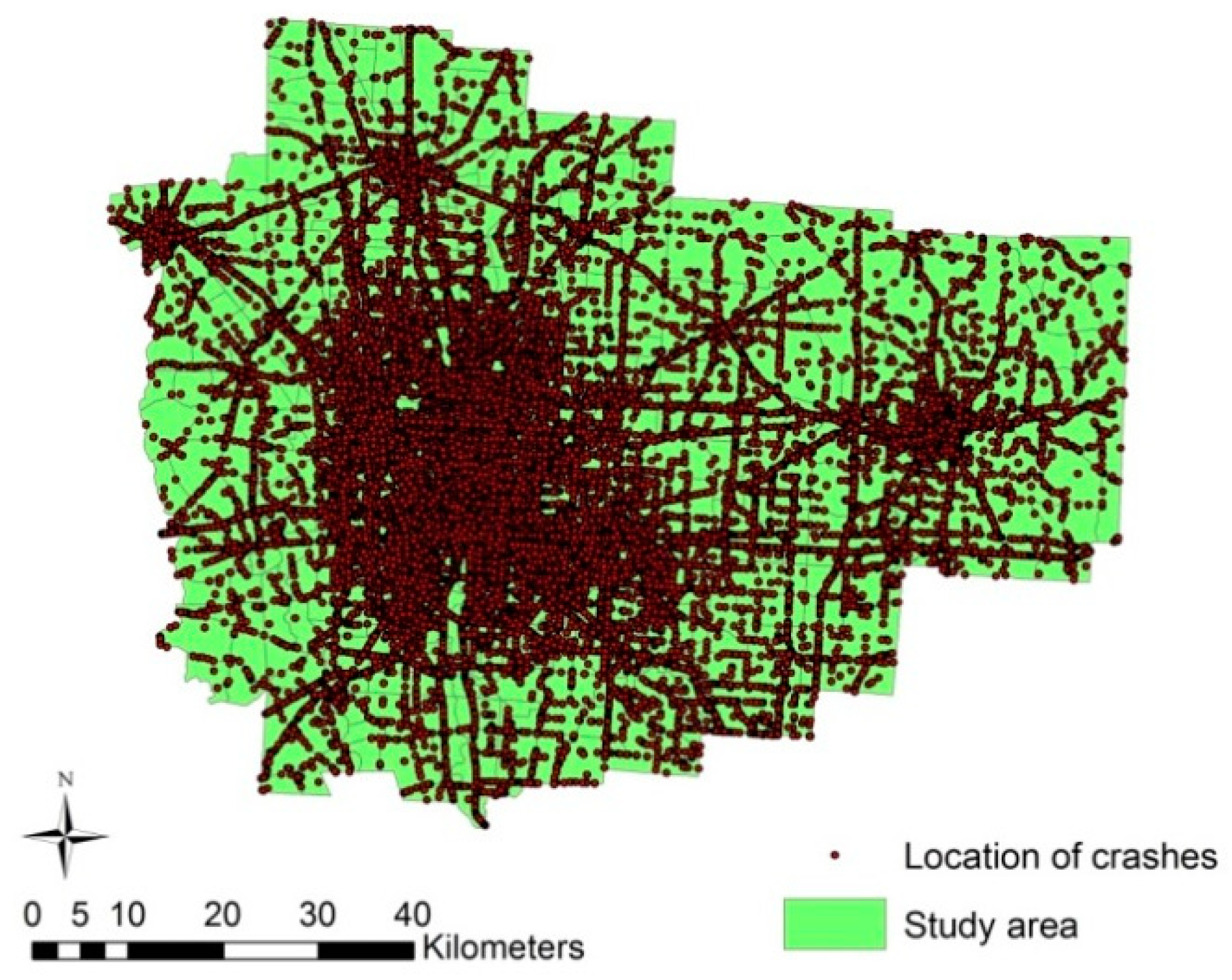
2.1. Study Area and Data

As Figure 1 indicates, the study area covers seven counties in the Columbus Metropolitan Area (CMA), the third-largest in Ohio, USA. All seven CMA counties were considered, but due to incomplete crash data, only four of them were included. Based on the 2010 census, the study area covered 2320 square miles, with a population of 1,654,374. The geographical unit is the traffic analysis zone (TAZ), with 1805 TAZs in the study area. A TAZ is one of the spatial units most commonly used for transportation planning models in the USA. Zones usually consist of one or more census blocks, block groups, or census tracks. The size of a zone varies according to traffic-related data and socio-economic data. Every year, around 300,000 crashes occur in Ohio, and about 15% of them occur in the study area.

The dataset was obtained from various sources.

Table 1. Source of data.

Category	Variable Name	Source
Crash Data	YDriver, MDriver, ODriver, Y06, Y07, Y08, Y09, Y10, and Y11	Ohio Department of Public Safety (ODPS)
Socio-Economic Factors	Popdensity, NHH, Empoff, HSchool, P1524, P5064, and Over65	Mid-Ohio Regional Planning Commission (MORPC) and U.S. Census of Population and Housing
Land-Use Factors	Residential and Commercial	County Auditors’ parcel-level data.
Public Transit and Traffic Flow Factors	Busstop, VMT, Road, and ASpeed,	Ohio Department of Transportation (ODOT), Central Ohio Transit Authority (COTA) and the Delaware Area Transit Authority (DATA)

shows the data source of each variable used in the study. The crash database was downloaded from the Ohio Department of Public Safety (ODPS), and categories were created for crash location, driver’s age, etc. To assess the impact of vehicle miles travel (VMT) on crashes, person trips per household per weekday data were drawn from the National Household Travel Survey (NHTS). The dependent variables are the number of crashes caused by young drivers, mature drivers, and older drivers per TAZ. Because of the need for comparability with other data, we used crash data over the period of 2006–2011. We determined the at-fault driver in a crash by an indicator of crash causation in the crash police report.

To investigate the relationship between crashes and the built environment, and socio-economic and demographic factors, we used a large volume of data on land use, demographics of current residents, employment, school enrollment, bus stop, average speed limit, etc.

Table 2. Descriptive statistics for the variables.

Variable	Description	Mean	SD	Minimum	Maximum
YDriver	Number of crashes caused by young drivers over the period 2006–2011 per TAZ	29.15	36.75	0	515
MDriver	Number of crashes caused by drivers aged 24–64 over the period 2006–2011 per TAZ	54.58	66.32	0	509
ODriver	Number of crashes caused by older drivers (65 +) over the period 2006–2011 per TAZ	6	7.5	0	64
Popdensity	Population Density (population/acre)	3.53	4.8	0	47.04
NHH	Number of households per TAZ	363.7	441.99	0	3248
Empoff	Office employment per TAZ	189.9	573.05	0	7729
HSchool	High school enrollment 2010 per TAZ	53.33	244.65	0	3103
P1524	Proportion of population between 15 and 24 years per TAZ	0.14	0.1	0	1
P5064	Proportion of population between 50 and 64 years per TAZ	0.2	0.07	0	1
Over 65	Proportion of population over 65 + years per TAZ	0.12	0.09	0	1
Residential	Proportion of residential land use per TAZ	0.3	0.27	0	0.96
Commercial	Proportion of commercial land use per TAZ	0.12	0.19	0	0.98
Busstop	Number of bus stops per TAZ	2.38	4.41	0	32
VMT	Vehicle miles per travel rate per weekday per TAZ	19.77	11.18	0	210.89
Road	Length of road (mile) per TAZ	4.55	4.73	0	43.14
Distance_C	Distance from the center of Columbus (mile) per TAZ	13.65	9.58	0.07	44.47
ASpeed	Average Speed of roads per TAZ	35.66	8.79	0	59.49
Y06	Number of crashes in 2006 per TAZ	13.3	17.7	0	151
Y07	Number of crashes in 2007 per TAZ	12.1	17.7	0	186
Y08	Number of crashes in 2008 per TAZ	16.5	17.7	0	192
Y09	Number of crashes in 2009 per TAZ	16	18	0	168
Y10	Number of crashes in 2010 per TAZ	15	20.18	0	138
Y11	Number of crashes in 2011 per TAZ	15	18.86	0	159

provides a description of the variables and basic statistics.

A total of 161,501 crashes occurred in the CMA during the period 2006–2011. The number of drivers, classified by age group, is presented in

Table 3. Crash frequency by driver groups (2006–2011).

Group	Crash Frequency	%
Young driver	52,093	32.3
Matured driver	98,526	61.0
Senior driver	10,882	6.7
Total	161,501	100.0

. We categorized drivers into three age groups. We designated young drivers as drivers aged between 15 and 24, based on an Organization for Economic Cooperation and Development (OECD) report [28], and older drivers as drivers aged 65 +, according to an American Automobile Association (AAA) report [29]. The other drivers, aged 25–64, were included in the mature driver group. Table 3 shows that 32.3% of all crashes were caused by young drivers, 61.0% by mature drivers, and 6.7% by senior drivers.

2.2. Statistical Analyses

We used statistical analyses to understand the relationship between the number of crashes and various factors at the macro level. Counting models were used, and the dependent variable was of the counting type. We used SAS (Statistical Analysis System), R, and Winbugs software to analyze the counting data. Based on the driver age group and statistical method, six models were developed.

Ordinary least squares (OLS), Poisson, and negative binomial (NB) models were commonly used in studies involving collision analysis. The OLS model is not appropriate in the case of nonlinearities, and zero values must be dropped when using logarithms. The Poisson model assumes that the mean-variance of the frequency of collisions is constant, but this assumption is often violated. As a result, we adopted a negative binomial model to control for the problems of overdispersion (presence of greater variability) or under dispersion (presence of less variability) based on the observed variance. This model was the preferred approach used in other crash frequency studies [24,25,30,31,32,33,34,35,36,37,38]. The Poisson model proved inadequate, but the negative binomial model proved to be appropriate. Therefore, we used the negative binomial model to regress the number of crashes on environmental and socio-economic factors. Using the negative binomial model implies that the mean and the variance are equal (E[y_i] = Var[y_i]). The variance of y_i is estimated using the mean crash frequency for entity i, with Var[y_i] = E[y_i][1 + α · E[y_i]] = E[y_i] + c · E[y_i]², where α is the overdispersion parameter, and c is a constant. The negative binomial model is expressed as lny_i = β’x_i + $\epsilon$, where x_i is the vector of independent variables. The estimated coefficient β’ represents the proportional change in the expected crash frequency from a unit change in the independent variables. However, this model does not account for any spatial dependence among spatial units such as TAZs.

To check for the existence of spatial autocorrelation (SA), the Moran’s I test has been widely used [30] and is used here to evaluate SA. In building the neighborhood matrix W, two locations (TAZs) that share an edge or a corner are considered neighbors, based on the queen adjacency of the first order. The results indicate that SA exists in all three models, as the Moran’s I indicator is significant at the 1% level in all models (See

Table 4. Results of the calculation of Moran’s I.

Group	Age Group	Moran’s I	p-Value
1	16 < age ≤ 24	0.36	<0.0001
2	24 < age ≤ 64	0.33	<0.0001
3	Over 65	0.31	<0.0001

).

Since the NB model cannot deal with the spatial dependency issue among adjacent spatial units, this study adopts the conditional autoregressive (CAR) model to deal with it. CAR models are widely used to represent spatial autocorrelation in various applications, including crash analysis [39]. Usually, the data are related to a set of non-overlapping areal units [40]. This model is presented below:

$$V_i ~ Poisson\left({\theta }_i\right)$$

(1)

$$ln{\theta }_i=\ln \left(E{V}_i\right) +\left({\beta }_0+ \beta x_i\right) + S{C}_i+U{H}_i$$

(2)

where $\beta$ is a vector of estimable coefficients representing the effects of the covariates, $E{V}_i$ is the exposure variable, and ${\beta }_0$ is the intercept term. $S{C}_i$ represents the spatial random effects (i.e., spatial correlation) as a conditional autoregressive (CAR) prior. $U{H}_i$ represents the unobserved (i.e., uncorrelated) heterogeneity.

The CAR model was implemented in a Bayesian setting, and inference was based on the Markov chain Monte Carlo (MCMC) simulation [40,41].

3. Analysis and Results

The number of observations is 1805 (number of TAZs in the study area). We expected the following directions of impacts of the independent variables: demographics (population density (+); number of households (+); proportions of the population between 15–24 (+), 50–64 (+), and over 65 (+)); socio-economic (high school enrollment (+)); built environment (proportion of commercial land use (+), number of bus stops (+), length of road (+), distance from the center of city (–)); average speed of roads (–); and the time variables Y06 (+), and Y07 (+), which show the number of crashes that occurred in 2006 and 2007.

Young driver, mature driver, and senior driver models were estimated with the negative binomial model. The results in

Table 5. Results of the negative binomial models.

Parameter	Description	Young Drivers	Mature Drivers	Senior Drivers
Intercept		3.14 (<0.0001) ***	3.715 (<0.0001) ***	1.774 (<0.0001) ***
Popdensity	Population Density (population /Acre)	- -	0.011 (0.017) **	- -
NHH	Number of Households	3 × 10−6 (<0.0001) ***	- -	- -
Empoff	Office Employment	0.0001 (0.005) ***	0.0001 (<0.0001) ***	0.0001 (0.0755) *
HSchool	High School Enrolment 2010	0.0003 (<0.0001) ***	- -	- -
P1524	Proportion of population between 15 and 24	0.786 (<0.0001) ***	- -	- -
P5064	Proportion of population between 50 and 64	–1.335 (<0.0001) ***	–1.138 (<0.0001) ***	- -
Over65	Proportion of population over 65	- -	- -	1.548 (<0.0001) ***
Commercial	Proportion of commercial land use	0.178 (0.0770) *	0.409 (<0.0001) ***	0.41 (<0.0001) ***
Busstop	Number of bus stop	- -	- -	0.021 (<0.0001) ***
VMT	Vehicle miles per travel rate per weekday	–0.001 (<0.0001) ***	–0.001 (0.0061) ***	–0.001 (<0.0001) ***
Road	Length of road (miles)	0.042 (<0.0001) ***	0.04 (<0.0001) ***	0.031 (<0.0001) ***
Distance_C	Distance from the center of Columbus (miles)	–0.007 (<0.0001) ***	–0.015 (<0.0001) ***	- -
ASpeed	Average Speed of roads	–0.022 (<0.0001) ***	–0.015 (< 0.0001) ***	–0.032 (<0.0001) ***
Y06	Crashes occurred in 2006	0.029 (<0.0001) ***	0.027 (<0.0001) ***	0.03 (<0.0001) ***
Y07	Crashes occurred in 2007	0.014 (<0.0001) ***	0.019 (<0.0001) ***	0.007 (0.0046) ***
Number of observations		1805	1805	1805
Number of parameters		12	10	9
DF		1792	1794	1795
${\mathrm{R}}_{\mathsf{\alpha }}^2$		0.67	0.64	0.68
Chi-squared goodness of fit test		0.844	0.954	0.384
Mean Pearson Chi-Square (value/DF)		0.966	0.944	1.01

p-values are in parentheses. * p < 0.10, ** p < 0.05, and *** p < 0.01.

indicate that 12 variables are significant for the young driver model, whereas 10 and 9 variables are significant for the mature driver and senior driver models, respectively. For the young drivers, demographic variables, such as the number of households, office employment, high school enrollment, proportion of population between 15 and 24, and proportion of population between 50 and 64, had significant impacts. Among the other variables, the proportion of commercial land use, length of road, distance from the center of Columbus (miles), average maximum speed of roads, and crashes that occurred in 2006 and 2007 were also significant. The vehicle miles per travel rate per weekday had a negative effect on the number of crashes caused by young drivers. For mature drivers, the population density, office employment, and proportion of population between 50 and 64 had a negative effect. Other variables display the same effects as for the young driver model, including VMT. Finally, the senior driver model shows that the number of crashes is positively influenced by office employment, the proportion of the population over 65, and the number of bus stops in a TAZ. Other variables showed the same trend as the previous two models, except for the distance from the center of Columbus variable. The number of crashes by senior drivers was negatively associated with VMT in the study area.

Table 5 shows the significant variables at the 95% level. According to Hadayeghi et al. [22], ${\mathrm{R}}_{\mathsf{\alpha }}^2$ = 1 − $\frac{\mathsf{\alpha }}{\mathsf{\alpha } \mathrm{intercept}}$ indicates the goodness-of-fit of the NB model. Notably, VMT is an important variable in the models for assessing the low-mileage bias. The VMT variable is strongly statistically significant in all models. In addition, the sign of VMT is negative not only in the senior driver model but also in the other two models. The number of households, office employment, high school enrollment, the proportion of population between 15 and 24, the proportion of commercial land use, and the length of road in the years 2006 and 2007 are significant with a positive sign. The proportion of population between 50 and 64, the distance from the center of Columbus, and the average maximum speed of roads are negatively associated with the number of crashes.

In the CAR models (

Table 6. Results of the CAR models.

Name	Young Drivers				Mature Drivers				Senior Drivers
	Mean	SD	2.5%	97.5%	Mean	SD	2.5%	97.5%	Mean	SD	2.5%	97.5%
Intercept	2.557	0.386	1.219	2.871	3.443	0.592	1.11	3.816	1.722	0.209	0.966	1.966
Popdensity	-	-	-	-	0.018	0.017	0.004	0.082	-	-	-	-
NHH	4.38 × 10−4	1.40 × 10−4	2.71 × 10−4	9.23 × 10−4	-	-	-	-	-	-	-	-
Empoff	9.68 × 10−5	3.79 × 10−5	4.63 × 10−5	1.76 × 10−4	1.52 × 10−4	5.42 × 10−5	7.19 × 10−5	3.08 × 10−4	6.02 × 10−4	4.02 × 10−5	6.24 × 10−6	1.56 × 10−4
HSchool	2.81 × 10−4	6.23 × 10−5	1.64 × 10−4	3.90 × 10−4	-	-	-	-	-	-	-	-
P1524	0.839	0.204	0.502	1.249	-	-	-	-	-	-	-	-
P5064	−0.9	0.336	−1.472	0.064	−0.696	0.348	−1.121	0.13	-	-	-	-
Over65	-	-	-	-	-	-	-	-	1.38	0.317	0.396	1.808
Commercial	0.323	0.11	0.131	0.529	0.433	0.131	0.218	0.787	0.43	0.114	0.181	0.626
Busstop	-	-	-	-	-	-	-	-	0.022	0.006	0.012	0.038
VMT	−6.2 × 10−4	3.2 × 10−5	−0.001	3.49 × 10−4	−5.69 × 10−4	5.68 × 10−4	−0.001	0.001	−0.001	4.01 × 10−4	−0.002	−5.37 × 10−4
Road	0.028	0.006	0.013	0.038	0.04	0.004	0.032	0.048	0.031	0.005	0.021	0.04
Distance_C	−0.005	0.002	−0.009	−5.14 × 10−4	−0.014	0.002	−0.018	−0.01	-	-	-	-
ASpeed	−0.009	0.007	−0.015	0.017	−0.011	0.012	−0.019	0.037	−0.03	0.005	−0.036	−0.009
Y06	0.027	0.003	0.023	0.033	0.028	0.003	0.023	0.036	0.03	0.003	0.025	0.036
Y07	0.015	0.002	0.01	0.02	0.018	0.002	0.013	0.023	0.007	0.003	0.002	0.012
SD of SC	0.29				0.24				0.25
SD of UH	0.81				0.82				0.86

), which address the spatial dependency issue, the results showed that there were few differences from those of the NB models. The results of the CAR models indicate that the signs of the coefficients of the independent variables are consistent with those of the NB models. The VMT variable in each model has a negative sign, consistent with that of the NB models. Demographic variables, socio-economic variables, and other variables are also the same in terms of the direction of effect.

4. Discussion

As our literature review has emphasized the existence of low-mileage bias, we have focused on the relationship between the number of crashes and VMT. The analysis of the NB and CAR model results shows that the relationship is inversely proportional. This can be interpreted as the possibility that being involved in crashes increases as people drive less. People driving less may have more chances of being involved in crashes than people who drive more. This is the same result as reported by Antin et al. [12], and Langford [8], who showed that low-mileage driver groups have higher crash rates when compared with medium-and high-mileage groups. As shown in Table 5 and Table 6, the low-mileage bias is not only found in the senior driver group but also in the other driver age groups. This result is not consistent with Pljakić et al. [42]. Unlike our results, they found that increasing Daily Vehicle-Kilometers Traveled increases the number of crashes.

Our results suggest that low-mileage issues exist in all age groups. The low-mileage bias has been argued to be due to aging, as prior literature has examined the nature of low-mileage bias only in terms of the characteristics of senior drivers. Plausible reasons may exist as to why driving less could lead to higher crash opportunities. In urban areas, everything is densely concentrated within the designated areas due to strict regulations and codes. Since many things are located close to residents’ homes, this may discourage people from driving long distances. Losing the opportunity to drive could decrease the ability to drive for all drivers. The complexity of the urban environment and the large number of vehicles can contribute to more crashes. However, several studies have attributed this phenomenon to the expedited loss of cognition through aging, although this might not only be true for senior drivers.

Aside from the biological characteristics of humans, this phenomenon might be related to urban road environments. Hence, we also examined the influence of the urban built environment on crash frequencies. The results confirm that demographics, socio-economic, and built-environment factors may also influence the chances of a crash occurring. The overall results support the idea that a more complex urban environment increases the likelihood of crashes. Population density contributes significantly to the number of crashes caused by drivers aged between 24 and 64. These results confirm the results of previous studies [24,31,35,43], except for Dumbaugh and Rae [33], who found that population density had a negative effect on the number of injury crashes. The number of household-occupied housing units has a positive and significant impact on crashes by young drivers. The larger number of housing units may be the result of higher housing density, fewer vacancies, or the exclusive use of dwelling compared to alternative land uses. In either case, there is more local residential activity, which explains the positive sign for this variable. High school enrollment might impact the driver composition by generating young drivers. This is the age where students learn to drive, purchase their first car, go to school, and attend other activities (such as parties). These results support Shope [44], who suggested that teenaged novice drivers were easily distracted and that their risk of crashing is higher than those for other age groups. High school environments involve high levels of bus and pedestrian activities and unexpected changes in speed that might impact drivers.

Our results show that the proportion of 15–24-year-old residents increases the crashes for young drivers. Dumbaugh and Rae [33] found that the population aged between 18 and 24 increased the number of collisions. A population below 15 may have a positive impact on the severity of pedestrian crashes, as shown by Clifton et al. [45]. This effect can be directly accounted for by the contribution of the resident population to this particular group of drivers. The data found in the literature are ambiguous about the impact of the aging population on crashes, which may perhaps be due to the lack of age-specific categorization and that few studies focused on faulty drivers. Quddus [38] showed those aged over 60 years in the population negatively impact the number of fatal injuries and minor injuries, but Wier et al. [46] showed that they contributed to vehicle–pedestrian collisions.

The results show that the proportion of people over 65 years in a TAZ may lead to more crashes involving the elderly. This may be related to the contribution of this group of residents to faulty elderly drivers. Crashes that occur in most age groups are positively and significantly affected by commercial land use. This result is consistent with Wier et al. [46], Pulugurtha et al. [36], and Kim et al. [24]. The number of bus stops positively impacts crashes across most age groups. As suggested by Lee et al. [17], bus stops may increase crash opportunities by increasing pedestrian flows and reducing visibility. The road length in the TAZ has a positive and significant impact in all models. The more roads that contain more vehicles, the greater the likelihood of collision. Previous studies [21,22,23,24,25,26,27,28,29,30,31,32,33,39] reported similar results. According to Kang [47], bus stops can substantially increase pedestrian volume, as well.

The results indicate that the distance from the center of Columbus has a negative impact on crashes caused by young and mature drivers. Central areas in cities can provide more collision targets (pedestrians, cars, etc.) than areas on the outskirts. However, Shi et al. [48] highlighted that high crash rates on rural roads could occur due to poorly designed road curves and the lack of traffic signs in China. The average speed limit of the TAZ has a negative and significant effect on the likelihood of crashes. This is an unexpected result because people usually expect that the number of crashes would decrease with the reduction of speed. One of the plausible reasons is that this study analyzed factors focusing on the number of crashes, not on their severity. Similar results have been reported in the literature. Blanco et al. [49] found similar results by using the Second Strategic Highway Research Program (SHRP2) Naturalistic Driving Study (NDS) data and stratified analysis. Quddus [38] also found that the mean speed (km/h) had a negative impact on the number of fatalities, injuries, and minor injuries. Bindra et al. [34] found that speed limits of less than 40 miles per hour had a negative impact on rural areas, but speed limits of less than 35 miles per hour had a positive impact in urban and suburban areas. Siddiqui et al. [37] found that a speed limit of 15 mph had a negative impact on pedestrian collisions.

We found spatial autocorrelation in the study area. Crashes that occur in the study area are spatially dependent and can be influenced by neighboring environments. There may be several reasons for that. Xu and Huang [39] suggested that the relationship between crash counts and surrounding environments is influenced by location due to intrinsically different relationships across the region, misspecification of reality, omitted relevant variables, and inappropriately represented the functional form. Lee et al. [17] suggested that several unobserved factors, such as road congestion, design, and materials of roads that were built in the same period and location, were spatially correlated. Also, Li et al. [50] discovered that the compactness of the urban environment is positively associated with traffic congestion.

5. Conclusions

We developed statistical models to investigate the relationship between driver groups classified by age and vehicle miles traveled. The outcomes from the structured models provided some reasonable answers to the research questions, which focused on the low-mileage bias. First, we confirmed that age groups besides older drivers were also associated with VMT, and that low mileage may contribute to more crashes regardless of driver age. Due to impairments caused by aging, such as visual and cognitive impairment, senior drivers have previously been targeted for this phenomenon, as compared with middle-aged and young drivers. However, the low-mileage bias was revealed not only in the crash model for senior drivers but also in the crash models for the other age groups. The results of this study suggest that low-mileage bias exists for senior drivers, drivers aged 25–64, as well as young drivers. The results imply that, regardless of age, driving less could lead to more chances of being involved in crashes.

Second, the results of the models support the hypothesis that the number of crashes and surrounding factors, such as the built environment and socio-economic and demographic factors, are closely related to each other. This was revealed not only in the results of the senior crash models but also in the models for the other age groups. We found influential urban environment factors (e.g., demographics, socio-economic factors, and built environment) on crashes, and the results were consistent with the literature in many cases, although some variables could not be applied to all age group, such as the composition of the population by age and high school enrollment. One plausible reason might be that a driver’s driving behavior is influenced by characteristics of the same or close age groups in the area. For example, in areas where high school enrollment is high, teenage novice drivers might contribute to more crashes.

Third, we found spatial autocorrelation in the study area, and we used CAR models to deal with this issue. We found few differences between the results of the NB models and those of the CAR models regarding the sign of the variables and their coefficient.

The average age of the total population is increasing due to an aging society. The above findings provide a better understanding of low-mileage bias and the determinants of crashes. This might assist decision makers in urban policy and planning to devise regulations and policies based on the behavior of drivers by age. Our findings also encourage more safety-emphasized planning, such as road management, to improve sustainable traffic safety by reducing the complexity of the driving environment and increasing overall neighborhood safety.

There are avenues to be addressed by future research. First, further analysis might be conducted based on crash severity and the driver’s age. Different types of damage caused by crashes may be differently associated with low-mileage bias. Second, follow up research regarding traffic safety policies should be conducted based on the characteristics of driver age and sex in addition to low-mileage bias, which will bridge the gap between the built environment and driving behaviors.

References

1. National Highway Traffic Safety Administration. Traffic Safety Fact 2018: 2016 Data; National Highway Traffic Safety Administration: Washington, DC, USA, 2018. [Google Scholar]
2. Cioca, L.I.; Ivascu, L. Risk indicators and road accident analysis for the Period 2012–2016. Sustainability 2017, 9, 1530. [Google Scholar] [CrossRef]
3. Li, G.; Braver, E.R.; Chen, L.H. Fragility versus excessive crash involvement as determinants of high death rates per vehicle mile of travel among older drivers. Accid. Anal. Prev. 2003, 35, 227–235. [Google Scholar] [CrossRef]
4. Massie, D.L.; Green, P.E.; Campbell, K.L. Crash involvement rates by driver gender and the role of average annual mileage. Accid. Anal. Prev. 1997, 29, 675–685. [Google Scholar] [CrossRef]
5. Janke, M.K. Accident, mileage, and the exaggeration of risk. Accid. Anal. Prev. 1991, 23, 183–188. [Google Scholar] [CrossRef]
6. Alvarez, F.J.; Fierro, I. Older drivers, medical condition, medical impairment and crash risk. Accid. Anal. Prev. 2008, 40, 55–60. [Google Scholar] [CrossRef]
7. Hanson, T.R.; Hildebrand, E.D. Area rural older drivers subject to low-mileage bias? Accid. Anal. Prev. 2011, 43, 1872–1877. [Google Scholar] [CrossRef]
8. Langford, J.; Methorst, R.; Hakamies-Blomqvist, L. Older drivers do not have a high crash risk: A replication of low mileage bias. Accid. Anal. Prev. 2006, 38, 574–578. [Google Scholar] [CrossRef] [PubMed]
9. Langford, J.; Koppel, S.; McCarthey, D.; Srinivasan, S. In defence of the low-mileage bias. Accid. Anal. Prev. 2008, 40, 1996–1999. [Google Scholar] [CrossRef] [PubMed]
10. Landford, J.; Charlton, J.L.; Koppei, S.; Myers, A.; Tuokko, H.; Marshall, S. Findings from the Candrive/Ozcandrive study; Low-mileage older drivers, crash risk and reduced fitness to drive. Accid. Anal. Prev. 2013, 61, 304–310. [Google Scholar] [CrossRef] [PubMed]
11. Staplin, L.; Gish, K.W.; Joyce, J. Low mileage bias and related policy implications-A cautionary note. Accid. Anal. Prev. 2008, 40, 1249–1252. [Google Scholar] [CrossRef]
12. Antin, J.F.; Guo, F.; Fang, Y.; Dingus, T.A.; Perez, M.A.; Hankey, J.M. A validation of the low mileage bias using naturalistic driving study data. J. Safety Res. 2017, 63, 115–120. [Google Scholar] [CrossRef] [PubMed]
13. Molnar, L.J.; Eby, D.W.; Bogard, S.E.; Leblanc, D.J.; Zakrajsek, J.S. Using naturalistic driving data to better understand the driving exposure and patterns of older drivers. Traffic Inj. Prev. 2018, 19, S83–S88. [Google Scholar] [CrossRef] [PubMed]
14. Regev, S.; Rolison, J.J.; Moutari, S. Crash risk by driver age, gender, and time of day using a new exposure methodology. J. Saf. Res. 2018, 66, 131–140. [Google Scholar] [CrossRef] [PubMed]
15. Rolison, J.J.; Moutari, S. Risk-Exposure density and mileage bias in crash risk for older drivers. Am. J. Epidemiol. 2018, 187, 53–59. [Google Scholar] [CrossRef] [PubMed]
16. Dumbaugh, E.; Zhang, Y. The relationship between community design and crashes involving older drivers and pedestrians. J. Plan. Educ. Res. 2013, 33, 83–95. [Google Scholar] [CrossRef]
17. Lee, D.; Guldmann, J.M.; Von Rabenau, B. Interactions between the built and socio-economic environment and driver demographics: Spatial econometric models of car crashes in the Columbus Metropolitan Area. Int. J. Urban Sci. 2018, 22, 17–37. [Google Scholar] [CrossRef]
18. Levine, N.; Kim, K. The location of motor vehicle crashes in Honolulu: A methodology for geocoding intersections. Comput. Environ. Urban. Syst. 1998, 22, 557–576. [Google Scholar] [CrossRef]
19. Fridstrom, L.; Ingebrigten, S. An aggregate accident model based on pooled, regional time-series data. Accid. Anal. Prev. 1991, 23, 363–378. [Google Scholar] [CrossRef]
20. Pawlovich, D.M.; Souleyrette, R.R.; Strauss, T. A Methodology for Studying Crash Dependence on Demographic and Socioeconomic data. In Proceedings of the Conference: Crossroads 2000, Iowa State University Ames, IA, USA, 19–20 August 1998; pp. 209–215. [Google Scholar]
21. Noland, R.; Oh, L. The effect of infrastructure and demographic change on traffic-related fatalities and crashes: A case study of Illinois county-level data. Accid. Anal. Prev. 2004, 36, 525–532. [Google Scholar] [CrossRef]
22. Hadayeghi, A.; Shalaby, A.S.; Persaud, B.N. Micro-Level accident prediction models for evaluating the safety of urban transportation systems. Transp. Res. Rec. 2003, 1840, 87–95. [Google Scholar] [CrossRef]
23. Guevara, F.L.; Washington, S.; Oh, J. Forecasting crashes at the planning level: Simultaneous negative binomial crash model applied in Tucson, Arizona. Transp. Res. Rec. 2004, 1897, 191–199. [Google Scholar] [CrossRef]
24. Kim, K.; Brunner, M.; Yamashita, E.Y. Influence of land use, population, employment and economic activity on accidents. Transp. Res. Rec. 2006, 1953, 56–64. [Google Scholar] [CrossRef]
25. Dumbaugh, E.; Li, W. Designing for the safety for pedestrians, cyclists, and motorists in urban environments. J. Am. Plann. Assoc. 2010, 77, 69–88. [Google Scholar] [CrossRef]
26. Hadayeghi, A.; Shalaby, A.; Persaud, B. Development of planning-Level transportation safety models using full bayesian semiparrametric additive techniques. J. Transp. Saf. Secur. 2010, 2, 45–68. [Google Scholar] [CrossRef]
27. Guo, Y.; Osama, A.; Sayed, T. A cross-Comparison of different techniques for modeling macro-Level cyclist crashes. Accid. Anal. Prev. 2018, 113, 38–46. [Google Scholar] [CrossRef] [PubMed]
28. International Transport Forum. Available online: https://www.itf-oecd.org/content/publication-0 (accessed on 20 March 2019).
29. American Automobile Association: Older Driver Fact Sheet. Available online: http://newsroom.aaa.com/wp-content/uploads/2012/11/SmartFeatures-FactSheet.pdf (accessed on 20 March 2019).
30. Cheng, Z.; Zu, Z.; Lu, J. Traffic crash evolution characteristic analysis and spatiotemporal hotspot identification of urban road intersections. Sustainability 2019, 11, 160. [Google Scholar] [CrossRef]
31. Graham, D.J.; Glaister, S. Spatial variation in road pedestrian casualties: The role of urban scale, density and land-Use mix. Urban Stud. 2003, 40, 1591–1607. [Google Scholar] [CrossRef]
32. Wedagama, D.M.P.; Bird, R.N.; Metcalfe, A.V. The influence of urban land-Use on non-Motorised trasport casulaties. Accid. Anal. Prev. 2006, 38, 1049–1057. [Google Scholar] [CrossRef]
33. Dumbaugh, E.; Rae, R. Safe urban form: Revisiting the relationship between community design and traffic safety. J. Am. Plann. Assoc. 2009, 75, 309–329. [Google Scholar] [CrossRef]
34. Bindra, B.; Ivan, N.J.; Jonsson, T. Predicting segment-Intersection crashes with land development data. Transp. Res. Rec. 2009, 2102, 9–17. [Google Scholar] [CrossRef]
35. Pulugurtha, S.S.; Sambhara, V.R. Pedestrian crash estimation models for signalized intersections. Accid. Anal. Prev. 2011, 43, 439–446. [Google Scholar] [CrossRef] [PubMed]
36. Pulugurtha, S.S.; Duddu, V.R.; Kotagiri, Y. Traffic analysis zone level crash estimation models based on land use characteristics. Accid. Anal. Prev. 2012, 50, 678–687. [Google Scholar] [CrossRef] [PubMed]
37. Siddiqui, C.; Abdel-Aty, M.; Choi, K. Macroscopic spatial analysis of pedestrian and bicycle crashes. Accid. Anal. Prev. 2011, 45, 382–391. [Google Scholar] [CrossRef] [PubMed]
38. Quddus, M.A. Modeling area-Wide count outcomes with spatial correlation and heterogeneity: An analysis of London crash data. Accid. Anal. Prev. 2008, 40, 1486–1497. [Google Scholar] [CrossRef] [PubMed] [Green Version]
39. Xu, P.; Huang, H. Modeling crash spatial heterogeneity: Random parameter versus geographically weighting. Accid. Anal. Prev. 2015, 75, 16–25. [Google Scholar] [CrossRef] [PubMed]
40. Lee, D. CARBayes: An R package for Bayesian spatial modeling with conditional autoregressive priors. J. Stat. Softw. 2013, 55, 1–24. [Google Scholar] [CrossRef] [Green Version]
41. Besag, J.; York, J.; Molli, E.A. Bayesian image restoration with two applications in spatial statistics. Annu. Inst. Stat. Math. 1991, 43, 1–59. [Google Scholar] [CrossRef]
42. Pljakic, M.; Jovanovic, D.; Matovic, B.; Micicc, S. Macro-Level accident modeling in Novi Sad: A spatial regression approach. Accid. Anal. Prev. 2019, 132, 105259. [Google Scholar] [CrossRef]
43. Wen, H.; Zhang, X.; Zeng, Q.; Lee, J.; Yuan, Q. Investigating Spatial Autocorrelation and Spillover Effects in Freeway Crash-Frequency Data. Int. J. Environ. Res. Public Health 2019, 16, 219. [Google Scholar] [CrossRef] [Green Version]
44. Shope, J.T. Influences on youthful driving behavior and their potential for guiding interventions to reduce crashes. Inj. Prev. 2006, 12, i9–i14. [Google Scholar] [CrossRef]
45. Clifton, K.J.; Fults, K.K. An examination of the environmental attributes associated with pedestrian-Vehicular crashes near public schools. Accid. Anal. Prev. 2007, 39, 708–715. [Google Scholar] [CrossRef] [PubMed]
46. Wier, M.; Weintraub, J.; Humphreys, E.H.; Seto, E.; Bhatia, R. An area-Level model of vehicle-Pedestrian injury collisions with implications for land use and transportation planning. Accid. Anal. Prev. 2009, 41, 137–145. [Google Scholar] [CrossRef] [PubMed]
47. Kang, C. The S+5Ds: Spatial access to pedestrian environments and walking in Seoul, Korea. Cities 2018, 77, 130–141. [Google Scholar]
48. Shi, L.; Huseynova, N.; Yang, B.; Li, C.; Gao, L. A cask evaluation model to assess safety in Chinese rural roads. Sustainability 2018, 10, 3864. [Google Scholar] [CrossRef] [Green Version]
49. Blanco, M.; Atwood, J.; Russell, S.; Trimble, T.; McClafferty, J.; Perez, M. Automated Vehicle Crash Rate Comparison Using Naturalistic Data 2016; Virginia Tech Transportation Institute: Blacksburg, VA, USA, 2016. [Google Scholar]
50. Li, Y.; Xiong, W.; Wang, X. Does polycentric and compact development alleviate urban traffic congestion? A case study of 98 Chinese cities. Cities 2019, 88, 100–111. [Google Scholar] [CrossRef]
Figure 1. Crash locations from 2006 to 2011 in the study area.
Sustainability 11 06643 g001