Grassland Productivity Response to Climate Change in the Hulunbuir Steppes of China

Abstract

As global climate change deeply affects terrestrial ecosystem carbon cycle, it is necessary to understand how grasslands respond to climate change. In this study, we examined the role of climate change on net primary productivity (NPP) from 1961 to 2010 in the Hulunbuir grasslands of China, using a calibrated process-based biogeochemistry model. The results indicated that: Temperature experienced a rise trend from 1961; summer and autumn precipitation showed a rise trend before the 1990s and decline trend after the 1990s. Winter and spring precipitation showed an ascending trend. Simulated NPP had a high inter-annual variability during the study period, ranging from 139 g Cm⁻² to 348 g Cm⁻². The annual mean NPP was significant and positive in correlation with the annual variation of precipitation, and the trend was first raised then fell with the turn point at the 1990s. Temperature had a 20–30 d lag in summer, but none in spring and autumn; precipitation had a 10–20 d lag in summer. The climate lag effect analysis confirmed that temperature had a positive effect on NPP in spring and a negative effect in summer.

1. Introduction

In response to anthropology causing rapidly rising concentrations of atmospheric greenhouse gases, the mean global temperature has increased continuously since the 1850s, with even higher rates after the 1950s [1]. Within the foreseeable future, anthropogenic climate change will lead to global warming and more variable precipitation. Warming directly influences the precipitation pattern, such as drier areas become drier and wet areas become wetter especially in the mid to high latitudes. Since warming leads to an increased risk of drought in summer, but more precipitation occurs with rain instead of snow and snow melts earlier in spring [2,3]. These changes have pronounced impacts on terrestrial ecosystems [4], and the response of terrestrial ecosystems to climate change has been a major research issue of global change [5]. Grasslands are one of the most widespread vegetation types in worldwide, covering 24 million km², nearly one-fifth of the world’s land surface [6]. It accounts for 40% of the total land area in the northern temperate zone of China [7]. Moreover, grassland vegetation is highly sensitive and vulnerable to climate change [8]. Previous work has found that significant climate change over the past 50 years in temperate grasslands in China has certainly affected the plant productivity and the carbon budget of this region [9]. Due to their complexity and diversity, the grasslands of Hulunbuir belonging to the middle latitude area, located in northeastern China, appear to be more sensitive to climate change, making this ecosystem uniquely suitable for studies of the effect of climate change on productivity.

Vegetation net primary production (NPP), defined as the carbon uptake by plant through photosynthesis, is a key measurement for the carbon cycle and feedback between terrestrial ecosystems and atmosphere [10,11,12]. NPP directly measures the energy flowing into an ecosystem, while integrating climatic, ecological, geochemical, and human influences on the biosphere [11,13]. Therefore, while NPP is an important indicator to reflect ecosystem performance [14,15], accurate estimation of NPP is critical to understanding the carbon dynamics within the atmosphere–vegetation–soil continuum and the response of terrestrial ecosystem to the future climate [16].

Ground based measurements of carbon dynamics in the grassland ecosystem is time-consuming and laborious, therefore needs an alternative model approach to achieve the measurement easier. In recent decades, numerous models were introduced to research the carbon balance of terrestrial ecosystems with changing environmental conditions [17], including statistical models (regression models) [18], remote sensing based models [19], and process models [10]. Remote sensing based models relied on historical image record that cannot be used to estimate vegetation NPP during eras when remote sensing data lacked, therefore the time span of most studies started in the 1980s [20,21,22,23]. It is necessary to require a biogeochemical process model for understanding or predicting the impacts of climate change (past or future) on vegetation dynamics. The Biome-BGC model, as a mechanistic biogeochemical process model, combines a series of plant biology and ecosystem dynamics function to simulate carbon, water, and nitrogen exchange between the pedosphere and atmosphere through vegetation, which is more sophisticated than statistical models [10,24]. After being parameterized, it could predict ecosystem NPP responses to climatic conditions without remote sensing images. Due to deriving it from the forest-BGC model, the Biome-BGC model was mainly applied to forest ecosystems simulation in early stage. In recent years, some studies reported that Biome-BGC was applied to herbaceous vegetation even crops [25,26,27], but no detail work has been reported in Hulunbuir grasslands.

In the present study, our aim is to: (1) Calibrate and localize the Biome-BGC model used in Hulunbuir grassland community based on field surveyed biomass data and remote sensing derived NPP; (2) investigate the evidence of NPP change and trends of typical grasslands under five decades of climate change; and (3) assess how climate change affects grasslands by determining the relationship between grassland growth and climate variables.

2. Material and Methods

2.1. Study Area

The study sites were dispersed in the Hulunbuir grassland, Inner Mongolia of China. (Figure 1). This area has a temperate continental climate driven by Asian monsoon, with mean annual precipitation of 255 mm (average during period of 1961–2010) and most of annual precipitation occurring from May to September. Mean annual temperature is about −0.5 ℃, while monthly mean temperature is about 19.8 ℃ in July and −23.3 ℃ in January. So that the hot and rainfall are in same period (Figure 2). The landforms from west to east are the Hulunbuir plateau, Great Khingan Mountain, and the west Nen river plain. Average elevation is 500–900 m above sea level. The native Hulunbuir ecosystem in the study area is high-quality grassland, representative of Mongolia, northern China. Vegetation in the study area mainly consists of arid steppe, meadow steppe, wetland and sandy vegetation. The community species of the region are comprised of Stipa baicalensis, Leymus chinensis, Stipa grandis, and Stipa krylovii. This area has a continental climate of the mid-latitude zone in the Mongolia plateau region, and local semiarid climate is deeply impacted by Siberian Mongolia cold and dry air [28].

2.2. Data Aquisition

Moderate resolution imaging spectroradiometer (MODIS) NPP production (MOD17A1) with spatial resolution 1 km was retrieved from NASA (https://lpdaac.usgs.gov). Land use and land cover (LUCC) dataset were introduced by WESTDC (2.0) which was produced by Cold and Arid Regions Environmental and Engineering Research Institute of China, National Natural Science Foundation of China (http://westdc.westgis.ac.cn). Meteorological data were acquired from the China Meteorological Data Sharing Service System (http://data.cma.cn/), including daily maximum temperature, daily minimum temperature, daily precipitation, and daily solar radiation. Soil texture was extracted from the harmonized world soil database (HWSD), which was developed by Food and Agriculture Organization of the United Nations (FAO) [29]. Historical CO₂ concentration data were adopted from the Global Greenhouse Gas reference Network of NOAA (www.esrl.noaa.gov/gmd/ccgg/trends). The atmospheric N deposition rate was derived from Zhu et al. [30]. Historical field grassland biomass measurements was acquired from the National Agriculture Science Data Sharing Center (http://grassland.agridata.cn/).

2.3. Model Simulation

2.3.1. Biome-BGC Model Description

Biome-BGC is a process-based mechanistic model that is used to simulate the storage and fluxes of water, carbon, and nitrogen within the vegetation, litter, and soil components of a terrestrial ecosystem with a daily time step [31]. The model originally was developed from Forest-BGC models, designed to describe seven natural biomes, including C3 and C4 grasses [32,33]. In this model, NPP was computed as the difference between gross photosynthesis and autotrophic respiration. Gross photosynthesis on a unit projected leaf area basis was estimated independently for the sunlit and shaded canopy fractions using the Farquhar photosynthesis routine [34]. The maximum rate of carboxylation was calculated as a function of the specific activity of the Rubisco enzyme (itself a function of leaf temperature), the weight fraction of nitrogen in Rubisco enzyme, the specific leaf area, and the leaf C:N ratio. Autotrophic respiration was the sum of maintenance and growth respiration of the different parts of the plant (canopy, stem, and roots). Maintenance respiration of each plant component was calculated as a function of tissue mass, tissue nitrogen concentration, and tissue temperature. Growth respiration was a simple proportion of total new carbon allocated to growth. More details of the modules description could be found in Thornton 2010 [35].

This model requires three types of datasets: Daily climate data (maximum and minimum temperature, precipitation, solar radiation, and vapor pressure deficit (VPD)), site parameters (i.e., soil texture, active soil depth, annual nitrogen deposition, elevation, latitude), and eco-physiological characteristics of vegetation parameters [36]. MTCLIM (version 4.3) was used to reprocess the daily meteorological data to match the Biome-BGC model data input [37,38].

2.3.2. Model Calibration

In the present work, we tuned eco-physiological parameters for adjusting model simulating processes referring to the site grass composition structure. Based on mechanisms of Biome-BGC modules described in the above section, we mainly refined the parameters that closely related to NPP simulation, such as allocation, maintenance, respiration, etc. Biome-BGC is considered a “big-leaf” model: It treats the landscape canopy as a single leaf layer with a given thickness and is neither individual nor species-based [39]. In the study area, grass community was composed of four constructive species (Stipa baicalensis, Leymus chinensis, Stipa grandis, and Stipa krylovii). We assumed that the “big-leaf” canopy was a homogeneous mixture of these species (averaging each species’ eco-physiological properties). Additionally, the eco-physiological parameters of each species were measured in the growing season at Xilin area [40]. We refined the parameter based on weighted average of characteristics of four species. Thus, the parameter settings for grasses will be adapted to conditions in Hulunbiur. Field measured grass biomass in the HLE region was used to assess the model performance. All field survey data were only collected aboveground the biomass enclosure plot in late August or beginning of September of each growing season, and no underground biomass of grass was measured. Therefore, we calculated the NPP by using the equations as follows [26,27]:

$$\mathrm{NPP}=D{M}_{AG}\times 0.45+D{M}_{BG}\times 0.36$$

(1)

$$\frac{D{M}_{AG}}{D{M}_{BG}}=\frac{1}{3}$$

(2)

where $D{M}_{AG}$ and $D{M}_{BG}$ indicate aboveground biomass (dry matter) and belowground biomass, respectively. 0.45 and 0.36 represent carbon content (gC/m²kg).

The root mean square error (RMSE) was used as an indice to evaluate the model performance when parameters tuning. The lower RMSE indicates higher accuracy of NPP estimate. After the manual tuning model, the optimized parameters were shown in

Table 1. Eco-physiological parameters for site community.

Eco-Physiological Parameters.	Values
Soil depth (m)	1 [40]
Annual leaf and fine root turnover fraction (1/a) *	1
New fine root C:new leaf C (ration) *	1.5
C:N of leaves (kgC/kgN) *	16.82
C:N of leaf litter (kgC/kgN) *	26
C:N of fine roots (kgC/kgN) *	30
Leaf litter labile proportion (DIM)	0.563
Leaf litter cellulose proportion (DIM)	0.369
Leaf litter lignin proportion (DIM)	0.068
Fine root labile proportion (DIM)	0.34
Fine root cellulose proportion (DIM)	0.44
Fine root lignin proportion (DIM)	0.22
Dead wood cellulose proportion (DIM)	0.75
Canopy water interception coefficient (1/d/LAI)	0.01
Canopy light extinction coefficient (DIM)	0.48
Canopy average specific leaf area (m2/kgC)	17.86
Maximum stomatal conductance (m/s)	0.006
Cuticular conductance (m/s)	0.00006
Boundary layer conductance (m/s)	0.04
Leaf water potential: start of conductance reduction (MPa)	−0.73
Leaf water potential: complete conductance reduction (MPa)	−2.7
VPD: start of conductance reduction (Pa)	1250.0
VPD: complete conductance reduction (Pa)	5000.0

* asterisk indicates the main eco-physiological parameter tuned in model calibration.

, and the model performance in HLE was depicted in Figure 3. Then, we initialized at all nine sites with the same set of eco-physiological parameters to simulate the NPP.

2.4. Model Validation of Other Sites

Without sufficient field-measured data, it is difficult to validate the model result in a regional scale. Here, the Biome-BGC simulations were compared with MODIS NPP which has been used for evaluating biomass or NPP dynamic of grassland [41,42,43]. In consideration of MODIS NPP based on remote sensing raster data, the LUCC raster mask was used to extract the grassland area of MODIS data. In order to calculate the regional mean NPP where the Biome-BGC site was located, we estimated the MODIS NPP derived as the median value of 10 × 10 km windows centered on each site.

2.5. Lag of Climate Effect on Grass NPP

In order to quantify the time lagged effects of climatic factors on grassland NPP, we divided each month during the growing season into thirds: First 10 days, second 10 days, third 10 days (for months of 28 or 31 days, the third period is defined as 8 or 11 days, respectively). We then calculated correlation coefficients for each 10 d NPP to climate factors (temperature and precipitation) averaged over the current 10 d and the previous four 10 d intervals. We identified the maximum value of these five coefficients as “peak lag”, which is the time period when the climate has the strongest effect on NPP (Figure 4).

2.6. Statistics

Temporal trends in the data variables were examined by the linear least squares regression and F-test was used for the significance testing. CV (coefficient of variation) is the ration of standard deviation and mean value, which evaluates temporal amplitude of variation. The anomaly was calculated from the time-series values minus averaged values and divided by these average values. Pearson correlation coefficient was applied to calculate the relation between two variables. Moving average method was applied to eliminate abnormal values for featuring trend in time series data. All statistics were carried out in the R program (version 3.4).

3. Result

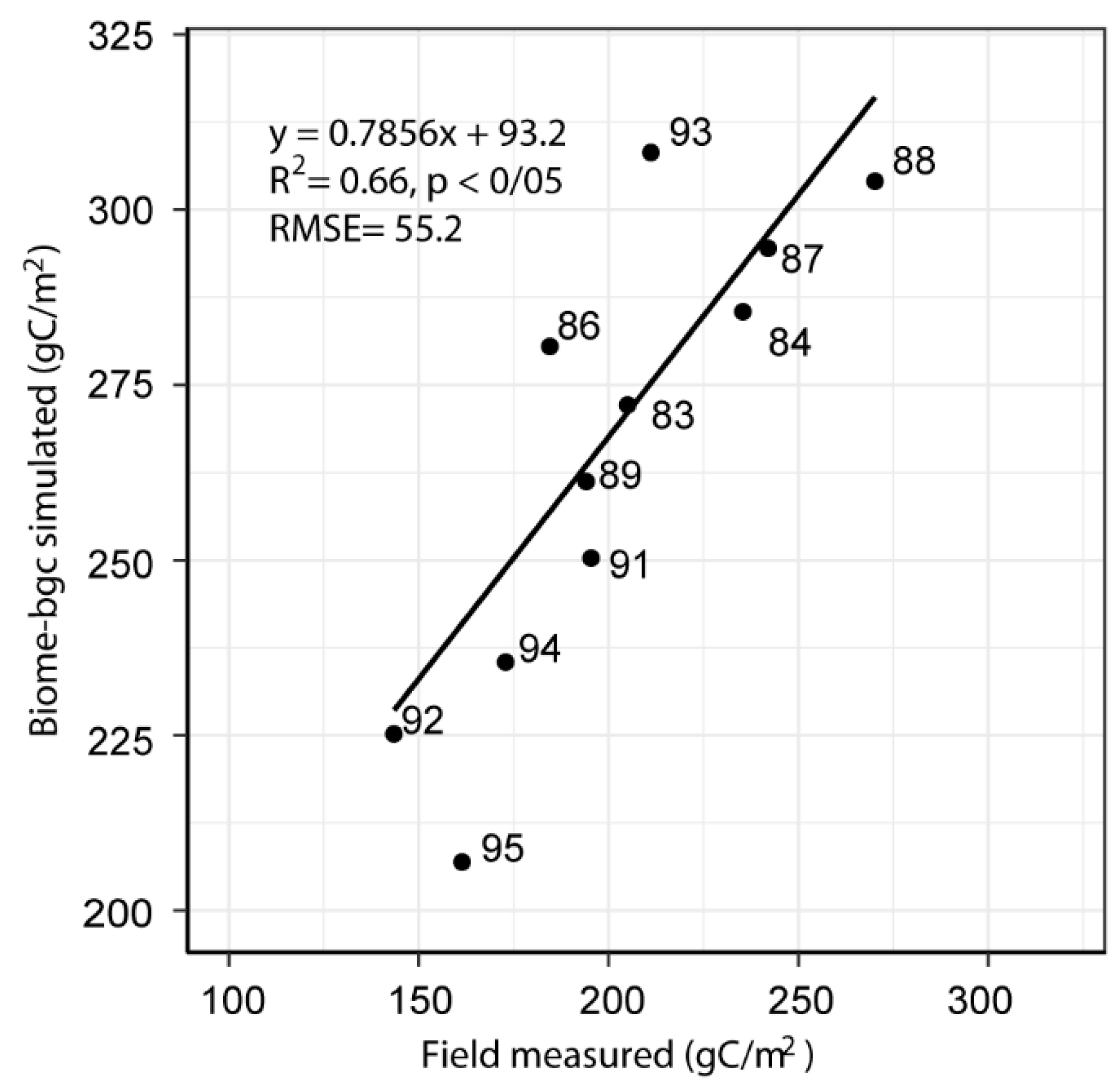
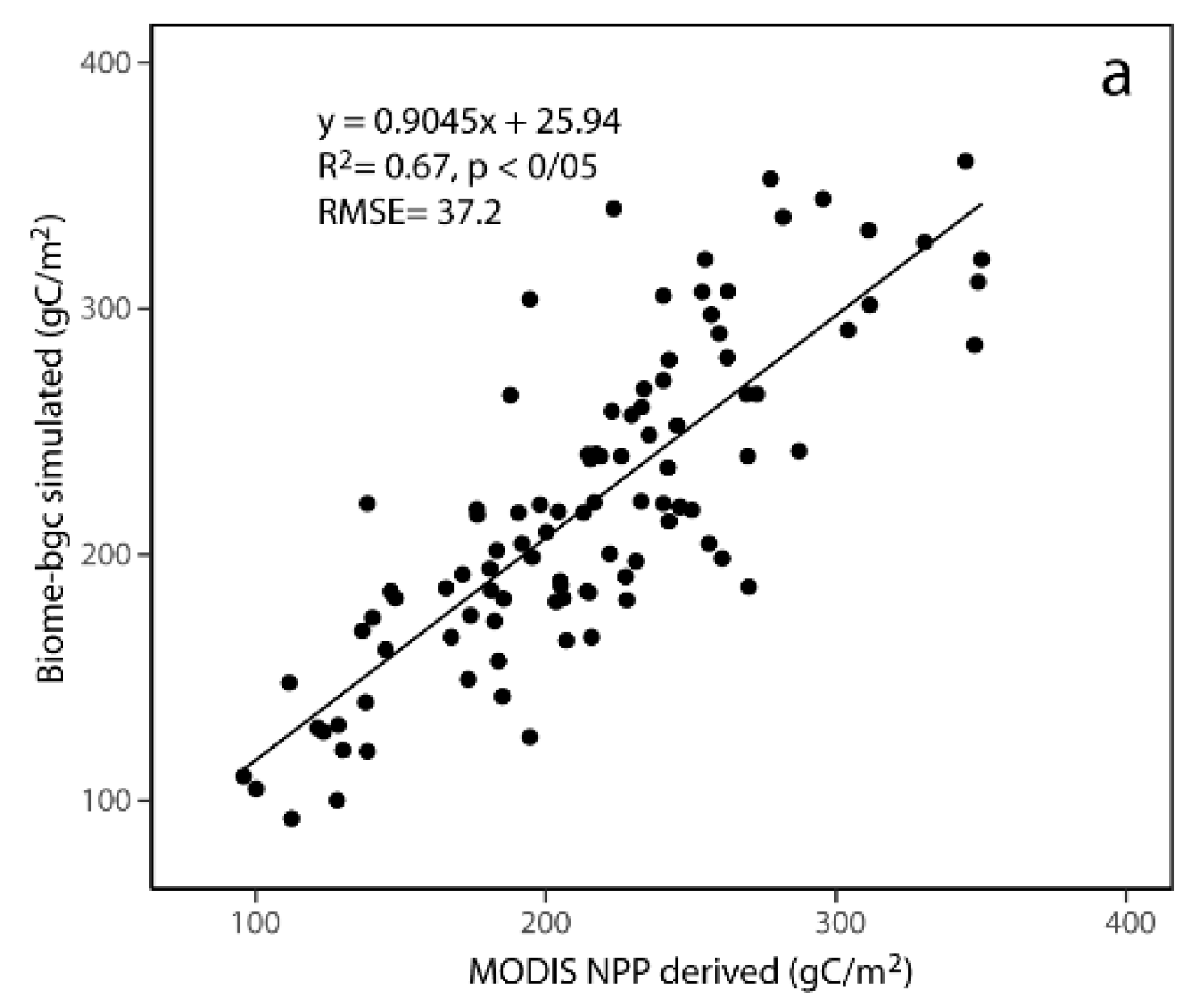
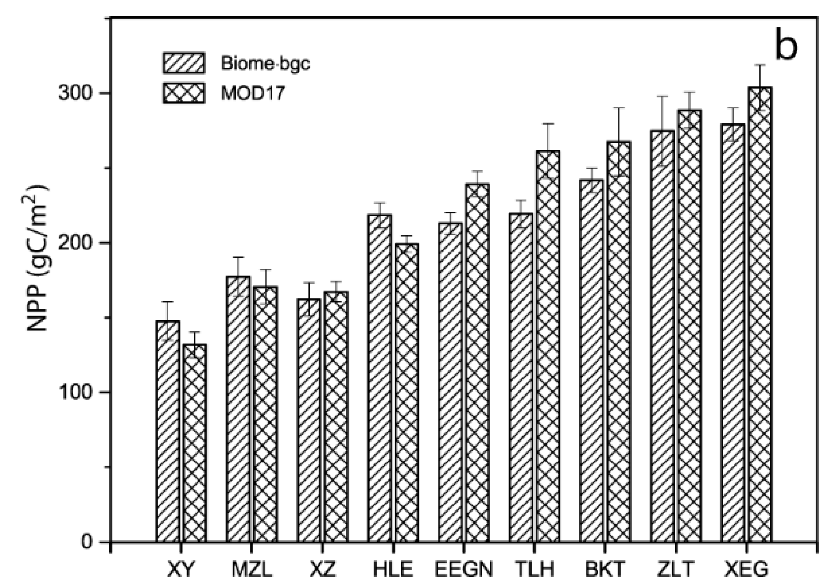
3.1. Model Validation

The comparison of Biome-BGC simulated NPP against MODIS NPP was shown in Figure 5a. The correlation coefficient suggested that Biome-BGC performed well in assessing the effect of climate on NPP in the study area (R² = 0.67, slope = 0.9045, p < 0.01). The comparison of multi-year mean NPP of each site was depicted in Figure 5b. The differences of Biome-BGC simulated and MODIS NPP are small and most of them showed as non-significant in statistics, which also indicates that the result of the simulation was reliable.

3.2. Trend of Climate Change

Across all sites, the annual accumulated temperature (AT) was monotonic significantly increasing at a rate of 8.12 °C/a with slight fluctuation. In contrast, there was no constant significant trend in annual precipitation (AP), but wide inter-annual variability was apparent (ranging from −33.1% to 77.8%), especially after the 1990s (Figure 6 and

Table 2. General characteristic of nine study sites and trends in AT, AP, and NPP.

Site.	Elevation	AT				AP					NPP
		Mean	Trend	CV	p	mean	range	CV	Trend	p	mean	range	CV	Trend	p
BKT	740	2253	5.2	0.05	<0.01	463	−52%–62%	0.19	−0.13	0.89	275	–37.1–39.0%	0.19	–0.26	0.60
EEG	581	2360	10.6	0.08	<0.01	356	−42%–52%	0.20	−0.33	0.67	246	–32.3–45.7%	0.20	–0.19	0.70
HLE	610	2549	8.8	0.06	<0.01	347	−64%–56%	0.22	0.93	0.24	235	–54.5–49.8%	0.21	0.67	0.14
MZL	662	2492	8.9	0.07	<0.01	284	−51%–107%	0.31	−1.51	0.09	209	–59.3–59.6%	0.23	–0.64	0.19
TLH	733	1903	5.2	0.06	<0.01	442	36%–47%	0.17	−0.81	0.30	240	–31.8–12.5%	0.10	–0.22	0.32
XEG	286	2586	9.1	0.06	<0.01	496	−42%–102%	0.23	0.85	0.46	299	–38.7–21.3%	0.13	–0.04	0.91
XY	554	2818	8.5	0.06	<0.01	241	−57%–145%	0.37	−0.81	0.38	196	–48.1–71.9%	0.27	–0.46	0.40
XZ	642	2745	8.0	0.06	<0.01	272	−54%–117%	0.29	−0.03	0.97	200	–44.2–68.2%	0.23	–0.28	0.53
ZLT	307	2972	8.8	0.05	<0.01	487	−56%–128%	0.27	0.47	0.73	296	–56.4–35.9%	0.19	–0.04	0.94

Note: Elevation (m); AT (°C) is accumulated temperature; AP (mm) is annual precipitation; mean indicated average of 50 years; CV is coefficient of variation; Trend is the slope of unary linear regression for past 50 years.

).

To assess the changes in each season, the five-year moving average temperature and precipitation from 1961 to 2010 were depicted in Figure 7. Temperature displayed a noticeable increasing trend for each season. The temperature of spring, summer, and autumn increased approximately 0.04 °C/a, while winter displayed a more rapid rising trend at 0.06 °C/a. Remarkably, summer and autumn temperatures have been warming dramatically at a rate of 0.082 and 0.068 °C/a, respectively since the beginning of the 1990s. Meanwhile, it is notable that precipitation increased in spring and winter and deceased in summer and autumn after the 1990s.

3.3. Dynamic Changes of NPP

Most of the sites showed that NPP slightly decreased but with no significant trend in the past five decades at all sites (Table 2). The inter-annual variation of averaged NPP of the nine sites are shown in Figure 6. Annual NPP exhibited inter-annual range variability in the past five decades and the amplitude of variation before the 1990s was larger than after the 1990s. NPP slightly increased to the highest point around the 1990s and then declined sharply. The annual mean NPP from highest to lowest are ZLT, XEG, BKT, TLH, EEG, HLE, MZL, XZ, XY, with a decreasing trend from southeast to northeast which was according to precipitation distribution, due to monsoon moisture decreasing from near coastal area to inland (Figure 1).

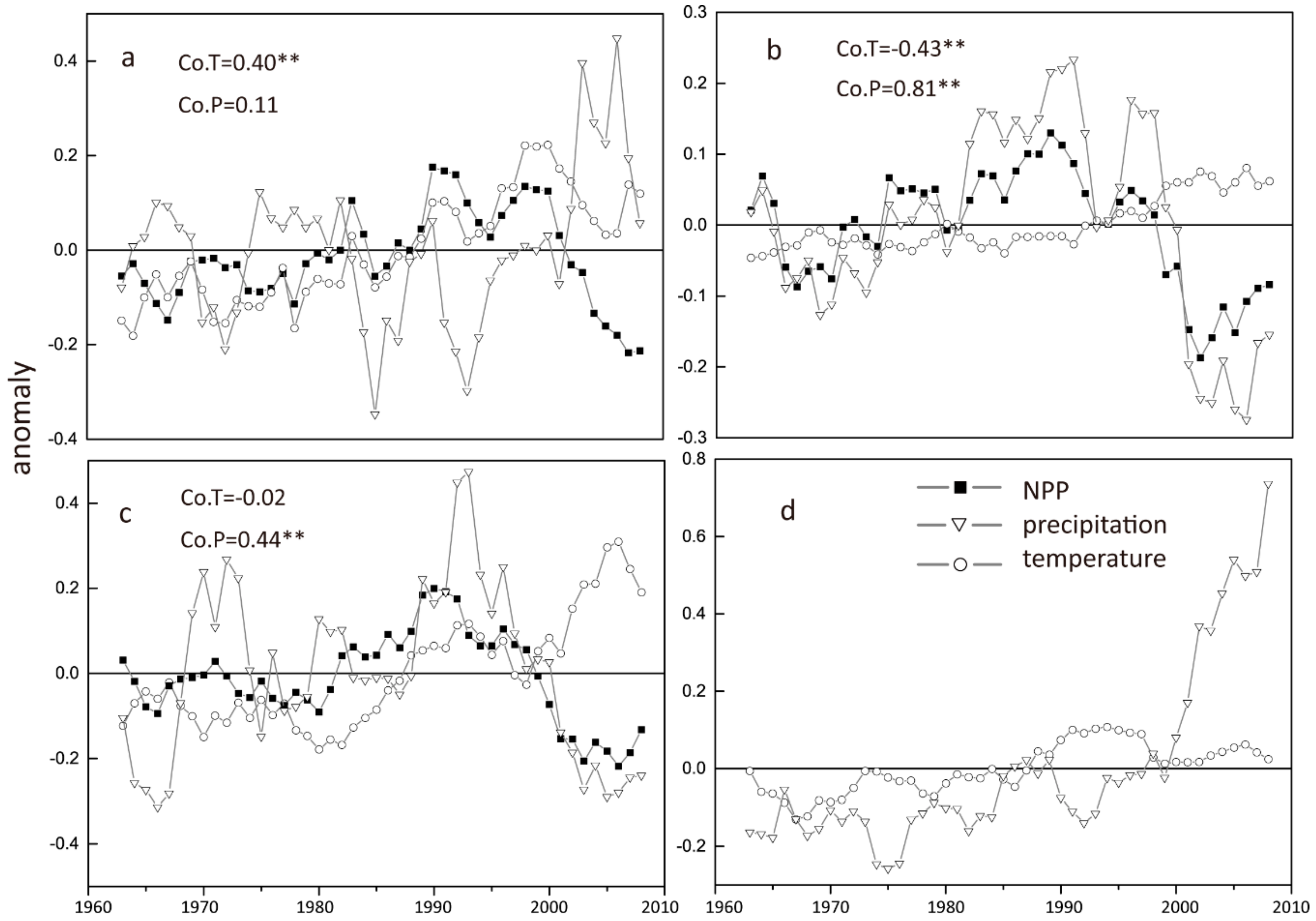
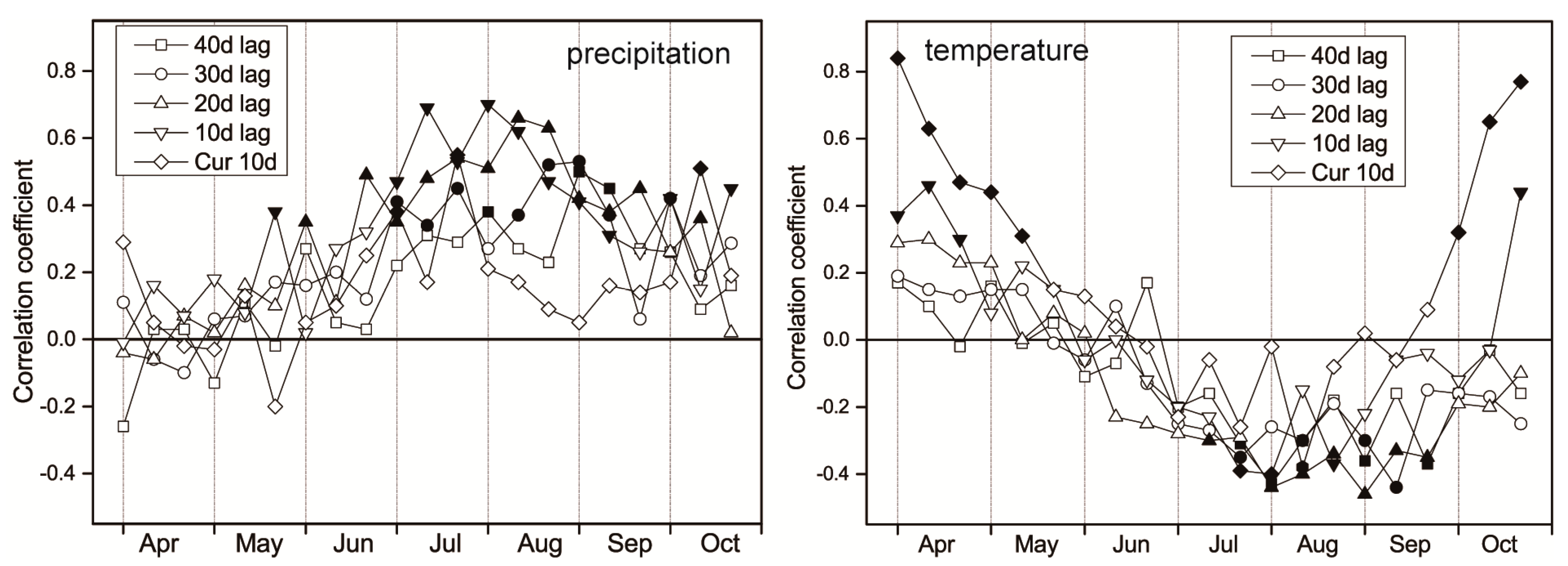
3.4. Lag Effect of Climate Factors

Temperature exhibited a negative effect on NPP in summer, while positive in spring and autumn (Figure 8). At the beginning and end of the growing season (April to May), the peak lag was short (0–10 d). In other words, current temperature directly impacted current grass growth in these periods. From mid-May to early July, the response of NPP to all time slices of temperatures was nonsignificant. From mid-July to September, there is a prominent lag in NPP response to temperature, and the lag length is overlapped. Unlike temperature, precipitation mainly exhibited a positive effect on NPP over the whole year, except for a weak negative correlation during the early growing season, and the significant lag effects emerge in June until the end of the growing season. The highest contemporaneous correlation coefficient has almost a 10 or 20 d lag.

4. Discussion

4.1. Model Validation

In this study, our simulations indicated that the Biome-BGC after optimized parameters is an appropriate model to estimate NPP of the Hulunbiur grassland ecosystem. The correlation of coefficient between field measured and simulated NPP was high (R² = 0.66) so that the accuracy of the simulation was in agreement with other studies [27,44,45]. Then, the simulated NPP by the parameterized Biome-BGC model was compared to MODIS NPP data. The result confirmed that the accuracy of the model is adequate in regional scale. The ability to accurately simulate the productivity of the study area supported us to analyze the long-term grassland carbon budget dynamics in response to historical climate change.

4.2. Response of Grassland NPP to Climate Change

The coefficient of correlation between annual NPP and precipitation was extremely significant (r = 0.82, p < 0.01), while with the annual mean temperature it was a nonsignificant correlation in the view of the whole region for the time period 1961–2010 (Figure 6). Comparing 50 years of annual NPP with temperature in each season, the results indicated that the climate factors impact of grass growth varies with seasons: The correlation coefficient of temperature and NPP are 0.41, −0.43, and −0.02 in spring, summer, and autumn, respectively; and the correlation coefficient of precipitation and NPP are 0.11, 0.81, and 0.44 in spring, summer, and autumn, respectively. Temperature and precipitation are both key factors influencing grasslands worldwide [46]. Temperature is a fundamental regulator of physiology and biochemistry processes. However, temperature effects on plant growth is complicated: On one side it can accelerate photosynthetic rates, enhance water use efficiency, and prolong the growing season; on the other side it can increase respiration, speeding up evapotranspiration that causes soil water stress [47]. In addition, warming temperature may increase the microbial decomposition N mineralization [48,49]. Our study indicated that temperature showed significant positive effects on grass growth in spring and significant negative effects in summer. Higher temperatures will enhance grass productivity in spring but reduce it in summer. AT, as the heat index of plant growth, was detected that the parallel rising global temperature was approximately at a rate of 8 °C/a [50]. This means that effective temperature during the growing season increased approximately 400 °C/a (nearly 17%) from 1961 to 2010. Although temperature has a weaker effect on annual NPP than precipitation, the effects of temperature on NPP could not be neglected [51,52,53]. Under global temperature continuously rising, many studies reported that plants have shifted to begin their growing season earlier in response to rising temperature in the northern hemisphere over the past several decades [54].

Precipitation is the essential limiting factor in arid and semi-arid regions [55,56]. Our results confirm that previous studies reported a significant and positive correlation between inter-annual variation of precipitation and NPP at site level studies [57,58]. In this study area, grass grows rapidly in summer when it is hot and rains at the same time, so that NPP in summer was approximately 60% proportionate in the current year, meanwhile that showed a strong relationship with the current season precipitation [59] (Figure 2). This means that precipitation from June to August is essential for grass growth. Zhang [5] researched the same conclusion in Inner Mongolia. Jobbagy and Sala [60] studied the relationship of grass aboveground NPP and precipitation in Patagonian steppe and suggested that the effect of seasonal precipitation on grass growth is more important than annual precipitation, which implies that grass growth concentrates on a relative short suitable physiological stage. Thus, the warming climate and decreased precipitation lead to soil moisture deficit, which may be the primary factor limiting grass productivity from the 1990s.

4.3. Lag Effects

Similar to its effect on inter-annual grass NPP, temperature exhibits two sides: Higher temperature directly stimulates grass growth in re-green stage and accelerates evapotranspiration causing water stress that restrains growth in summer. Water is not a primary limitation in the beginning of the growing season because water availability could be supplemented by thawing frozen snow/earth in cooler and wetter regions at meadow steppe. Additionally, grass is sensitive to temperature at this stage. Therefore, temperature is the basic environment factor. On the other hand, water consumption by grass is low at the beginning of the growth period because the grass leaves are small with lower evapotranspiration. Thus, the temperature peak lag is less than 10 d and there is no significant correlation with precipitation early in the growing season. Shen [61] found analogous results in cooler and wetter regions, which can explain that grass growth has no significant correlation to precipitation in the re-greening stage. Zhang [62] noted that both ecosystem photosynthesis and respiration have closer relationships with temperature in the early months of the growing season at a 10 d scale, which is in agreement with our results.

In the summer, excessive heat accelerates evapotranspiration resulting in a soil moisture deficit, which indirectly affects plants as a negatively limiting factor. Generally, there is a time lag for rainfall to be utilized, as the rainfall moves through the soil, absorbed by the roots, and finally used by the plant body. On the contrary, heat-driven water stress has a longer lag time due to the water-holding capacity of the soil. This could explain why precipitation showed 10–20 d lag, while temperature had a 20–30 d lag in summer. This finding reinforces the concept that precipitation is a major limiting factor influencing biomass in arid and semi-arid grassland ecosystems [63,64].

4.4. Uncertainty

Field harvest measurement was widely used to model validation [27,59,65]. In general, the field biomass measurements that represented NPP depends on the number of samples and the homogeneity of field vegetation. More attention was paid to choose homogeneous field samples that represented a wider area with similar vegetation growth, coverage, and species mixture ration, which played a significant role on model calibration. That is one of the reasons reliable remote sensing derived NPP data were introduced as auxiliary data for spatial validation [42]. Another uncertainty is that the best model parameters group for target site simulation is hard to obtain. The parameters optimization deeply depends on experts experience [66]. We just tuned model accuracy that was acceptable. In future study, machine learning algorithm should be applied in model calibration, for searching best parameter groups [67]. Lastly, the responses of grassland growth NPP to climate changes are the product of complicated interactions among environment factors, such as nitrogen deposition changes, human disturbance, and land use change [68,69]. It is necessary to integrate these factors for improving the precision of the model and that could apply on short-term simulation.

5. Conclusions

In this study, a mechanic biogeochemical model was calibrated under the parameters optimization framework, localized to estimate NPP of grassland in Hulunbuir, and examined the carbon dynamics and its response to climate change in a long-term period (1961–2010). In the view of the whole region, NPP exhibited substantial yearly variation and slightly ascending trend before the 1990s while descending after the 1990s. Precipitation was a dominant factor affecting NPP variation, while rising temperature promoted grass growth in spring and restrained it in the summer. The lag effect analysis reinforced the relationship between NPP and climate factors. In summary, this study provided a profound understanding of grassland growth response to climate change through reestablishment of carbon dynamic in the past decades by using a mechanic model, which could serve as a scientific reference for rational utilization and management of the pasture.

References

1. IPCC. The Physical Science Basis. Contribution of Working Group Ι to the Fourth Assessment Report of the Intergrovernmental Panel on Climate Change; Cambrudge University Press: Cambridge, UK, 2007.
2. IPCC. IPCC Fifth Assessment Synthesis Report; IPCC: Geneva, Switzerland, 2014.
3. Trenberth, K.E. Change in precipitation with climate change. Clim. Res. 2011, 47, 123–138. [Google Scholar] [CrossRef]
4. Ni, J. Estimating net primary productivity of grasslands from field biomass measurements in temperate northern China. Plant Ecol. 2004, 174, 217–234. [Google Scholar] [CrossRef]
5. Zhang, G.; Kang, Y.; Han, G.; Sakurai, K. Effect of climate change over the past half century on the distribution, extent and NPP of ecosystems of Inner Mongolia. Glob. Chang. Biol. 2011, 17, 377–389. [Google Scholar] [CrossRef]
6. Lieth, H. Patterns of Primary Productivity in the Biosphere. In Patterns of Primary Productivity in the Biosphere; Dowden, Hutchinson and Ross Inc.: Stroudburg, PA, USA, 1978. [Google Scholar]
7. Sun, H. Ecosystems of China; Science Press: Beijing, China, 2005. [Google Scholar]
8. Guisan, A.; Theurillat, J.P. Assessing alpine plant vulnerability to climate change: A modeling perspective. Integr. Assess. 2000, 1, 307–320. [Google Scholar] [CrossRef]
9. Chen, Z.; Wang, S. Typical Steppe Ecosystems of China; Science Press: Beijing, China, 2000. [Google Scholar]
10. Cramer, W.; Kicklighter, D.W.; Bondeau, A.; Iii, B.M.; Churkina, G.; Nemry, B.; Ruimy, A.; Schloss, A.L.; The Participants of The Potsdam NPP Model Intercomparison. Comparing global models of terrestrial net primary productivity (NPP): Overview and key results. Glob. Chang. Biol. 1999, 5, 1–15. [Google Scholar] [CrossRef]
11. Nemani, R.R. Climate–Driven Increases in Global Terrestrial Net Primary Production from 1982 to 1999. Science 2003, 300, 1560–1563. [Google Scholar] [CrossRef]
12. Running, S.W.; Baldocchi, D.D.; Turner, D.P.; Gower, S.T.; Bakwin, P.S.; Hibbard, K.A. A Global Terrestrial Monitoring Network Integrating Tower Fluxes, Flask Sampling, Ecosystem Modeling and EOS Satellite Data. Remote Sens. Environ. 1999, 70, 108–127. [Google Scholar] [CrossRef]
13. Williams, J.W.; Seabloom, E.W.; Slayback, D.; Stoms, D.M.; Viers, J.H. Anthropogenic impacts upon plant species richness and net primary productivity in California. Ecol. Lett. 2005, 8, 127–137. [Google Scholar] [CrossRef]
14. Lobell, D.B.; Hicke, J.A.; Asner, G.P.; Field, C.B.; Tucker, C.J.; Los, S.O. Satellite estimates of productivity and light use efficiency in United States agriculture, 1982–1998. Glob. Chang. Biol. 2002, 8, 722–735. [Google Scholar] [CrossRef]
15. Roy, J.; Saugier, B.; Mooney, H.A. Terrestrial Global Productivity. Austral Ecol. 2002, 27, 584–585. [Google Scholar]
16. Donmez, C.; Berberoglu, S.; Forrest, M.; Cilek, A.; Hickler, T. Comparing Process–Based Net Primary Productivity Models in a Mediterranean Watershed. ISPRS Int. Arch. Photogramm. Remote Sens. Spat. Inf. Sci. 2013, XL–7/W2, 67–74. [Google Scholar] [CrossRef]
17. Hidy, D.; Barcza, Z.; Haszpra, L.; Churkina, G.; Pintér, K.; Nagy, Z. Development of the Biome–BGC model for simulation of managed herbaceous ecosystems. Ecol. Model. 2012, 226, 99–119. [Google Scholar] [CrossRef]
18. Yuan, W.; Liu, S.; Zhou, G.; Zhou, G.; Tieszen, L.L.; Baldocchi, D.; Bernhofer, C.; Gholz, H.; Goldstein, A.H.; Goulden, M.L.; et al. Deriving a light use efficiency model from eddy covariance flux data for predicting daily gross primary production across biomes. Agric. For. Meteorol. 2007, 143, 189–207. [Google Scholar] [CrossRef]
19. Zhang, M.; Lal, R.; Zhao, Y.; Jiang, W.; Chen, Q. Estimating net primary production of natural grassland and its spatio–temporal distribution in China. Sci. Total Environ. 2016, 553, 184–195. [Google Scholar] [CrossRef] [PubMed]
20. Gao, Q.; Wan, Y.; Li, Y.; Guo, Y.; Ganjurjav; Qin, X.; Jiangcun, W.; Wang, B. Effects of topography and human activity on the net primary productivity (NPP) of alpine grassland in northern Tibet from 1981 to 2004. Int. J. Remote Sens. 2013, 34, 2057–2069. [Google Scholar] [CrossRef]
21. Feng, X.; Liu, G.; Chen, J.M.; Chen, M.; Liu, J.; Ju, W.M.; Sun, R.; Zhou, W. Net primary productivity of China’s terrestrial ecosystems from a process model driven by remote sensing. J. Environ. Manag. 2007, 85, 563–573. [Google Scholar] [CrossRef]
22. Liu, Y.; Ju, W.; He, H.; Wang, S.; Sun, R.; Zhang, Y. Changes of net primary productivity in China during recent 11 years detected using an ecological model driven by MODIS data. Front. Earth Sci. 2013, 7, 112–127. [Google Scholar] [CrossRef]
23. Wang, H.; Prentice, I.C.; Ni, J. Primary production in forests and grasslands of China: Contrasting environmental responses of light– and water–use efficiency models. Biogeosciences 2012, 9, 4689–4705. [Google Scholar] [CrossRef]
24. Vetter, M.; Churkina, G.; Jung, M.; Reichstein, M.; Zaehle, S.; Bondeau, A.; Chen, Y.; Ciais, P.; Feser, F.; Freibauer, A.; et al. Analyzing the causes and spatial pattern of the European 2003 carbon flux anomaly using seven models. Biogeosciences 2008, 5, 561–583. [Google Scholar] [CrossRef]
25. Barcza, Z.; Haszpra, L.; Somogyi, Z.; Hidy, D.; Lovas, K.; Churkina, G.; Horvath, L. Estimation of the biospheric carbon dioxide balance of Hungary using the BIOME–BGC model. Idojárás 2009, 113, 203–219. [Google Scholar]
26. Maselli, F.; Argenti, G.; Chiesi, M.; Angeli, L.; Papale, D. Simulation of grassland productivity by the combination of ground and satellite data. Agric. Ecosyst. Environ. 2013, 165, 163–172. [Google Scholar] [CrossRef]
27. Sun, Q.; Li, B.; Zhang, T.; Yuan, Y.; Gao, X.; Ge, J.; Li, F.; Zhang, Z. An improved Biome–BGC model for estimating net primary productivity of alpine meadow on the Qinghai–Tibet Plateau. Ecol. Model. 2017, 350, 55–68. [Google Scholar] [CrossRef]
28. Lv, S.; Liu, J.; Zheng, Z.; Ye, S.; Chang, X. Effects of the Annual Precipitation Fluctuation on Primary Productivity in Hulunbeier. Res. Environ. Sci. 2015, 4, 550–558. [Google Scholar]
29. Nachtergaele, F.; van Velthuizen, H.; Verelst, L. Harmonized World Soil Database, Food and Agriculture Organization of the United Nations; FAO: Roma, Italy, 2009. [Google Scholar]
30. Zhu, J.; He, N.; Wang, Q.; Yuan, G.; Wen, D.; Yu, G.; Jia, Y. The composition, spatial patterns, and influencing factors of atmospheric wet nitrogen deposition in Chinese terrestrial ecosystems. Sci. Total Environ. 2015, 511, 777–785. [Google Scholar] [CrossRef]
31. Running, S.W.; Hunt, E.R. Generalization of a Forest Ecosystem Process Model for Other Biomes, BIOME–BGC, and an Application for Global–Scale Models. In Scaling Physiological Processes; Roy, J., Ehleringer, J.R., Field, C.B., Eds.; Academic Press: San Diego, CA, USA, 1993; pp. 141–158. ISBN 978-0-12-233440-5. [Google Scholar]
32. Running, S.W.; Gower, S.T. FOREST–BGC, A general model of forest ecosystem processes for regional applications. II. Dynamic carbon allocation and nitrogen budgets. Tree Physiol. 1991, 9, 147–160. [Google Scholar] [CrossRef]
33. White, M.A.; Thornton, P.E.; Running, S.W.; Nemani, R.R. Parameterization and Sensitivity Analysis of the BIOME–BGC Terrestrial Ecosystem Model: Net Primary Production Controls. Earth Interact. 2000, 4, 1–85. [Google Scholar] [CrossRef]
34. Farquhar, G.D.; von Caemmerer, S.; Berry, J.A. A biochemical model of photosynthetic CO2 assimilation in leaves of C3 species. Planta 1980, 149, 78–90. [Google Scholar] [CrossRef]
35. Thornton, P.E.; Running, S.W. Theoretical Framework of Biome–BGC Version4.2; Technical Documentation: Missoula, MT, USA, 2010. [Google Scholar]
36. Running, S.W.; Coughlan, J.C. A General Model of Forest Ecosystem Processes for Regional Applications I. Hydrologic Balance, Canopy GAS Exchange and Primary Production Processes. Ecol. Model. 1988, 42, 125–154. [Google Scholar] [CrossRef]
37. Bohn, T.J.; Livneh, B.; Oyler, J.W.; Running, S.W.; Nijssen, B.; Lettenmaier, D.P. Global evaluation of MTCLIM and related algorithms for forcing of ecological and hydrological models. Agric. For. Meteorol. 2013, 176, 38–49. [Google Scholar] [CrossRef]
38. Potter, C.S.; Randerson, J.T.; Field, C.B.; Matson, P.A.; Vitousek, P.M.; Mooney, H.A.; Klooster, S.A. Terrestrial ecosystem production: A process model based on global satellite and surface data. Glob. Biogeochem. Cycles 1993, 7, 811–841. [Google Scholar] [CrossRef]
39. Boisvenue, C.; Running, S.W. Simulations show decreasing carbon stocks and potential for carbon emissions in Rocky Mountain forests over the next century. Ecol. Appl. 2010, 20, 1302–1319. [Google Scholar] [CrossRef] [PubMed]
40. Dong, M.; Yu, M. Simulation analysis on net primary productivity of grassland communities along a water gradient and their responses to climate change. J. Plant Ecol. 2008, 32, 531–543. [Google Scholar]
41. Zhang, L.; Wylie, B.K.; Ji, L.; Gilmanov, T.G.; Tieszen, L.L. Climate-Driven Interannual Variability in Net Ecosystem Exchange in the Northern Great Plains Grasslands. Rangel. Ecol. Manag. 2010, 63, 40–50. [Google Scholar] [CrossRef]
42. Reeves, M.C.; Moreno, A.L.; Bagne, K.E.; Running, S.W. Estimating climate change effects on net primary production of rangelands in the United States. Clim. Chang. 2014, 126, 429–442. [Google Scholar] [CrossRef]
43. Heinsch, F.A.; Zhao, M.; Running, S.W.; Kimball, J.S.; Nemani, R.R.; Davis, K.J.; Bolstad, P.V.; Cook, B.D.; Desai, A.R.; Ricciuto, D.M.; et al. Evaluation of remote sensing based terrestrial productivity from MODIS using regional tower eddy flux network observations. IEEE Trans. Geosci. Remote. Sens. 2006, 44, 1908–1925. [Google Scholar] [CrossRef] [Green Version]
44. Maselli, F.; Chiesi, M.; Moriondo, M.; Fibbi, L.; Bindi, M.; Running, S.W. Modelling the forest carbon budget of a Mediterranean region through the integration of ground and satellite data. Ecol. Model. 2009, 220, 330–342. [Google Scholar] [CrossRef]
45. Han, Q.; Luo, G.; Li, C.; Ye, H.; Chen, Y. Modeling grassland net primary productivity and water–use efficiency along an elevational gradient of the Northern Tianshan Mountains. J. Arid Land 2013, 5, 354–365. [Google Scholar] [CrossRef] [Green Version]
46. Bai, Y.; Wu, J.; Xiang, Q.; Pan, Q.; Huang, J.; Yang, D.; Han, X. Primary production and rain use efficiency across a precipitation gradient on the mongolia plateau. Ecology 2008, 89, 2140–2153. [Google Scholar] [CrossRef]
47. Tatarinov, F.A.; Cienciala, E. Long–term simulation of the effect of climate changes on the growth of main Central–European forest tree species. Ecol. Model. 2009, 220, 3081–3088. [Google Scholar] [CrossRef]
48. Dai, L.; Ke, X.; Du, Y.; Zhang, F.; Li, Y.; Li, Q.; Lin, L.; Peng, C.; Shu, K.; Cao, G.; et al. Nitrogen controls the net primary production of an alpine Kobresia meadow in the northern Qinghai–Tibet Plateau. Ecol. Evol. 2019, 9, 8865–8875. [Google Scholar] [CrossRef] [Green Version]
49. Gao, W.; Yan, D. Warming suppresses microbial biomass but enhances N recycling. Soil Biol. Biochem. 2019, 131, 111–118. [Google Scholar] [CrossRef]
50. Ren, J.Z.; Hu, Z.Z.; Zhao, J.; Zhang, D.G.; Hou, F.J.; Lin, H.L.; Mu, X.D. A grassland classification system and its application in China. Rangeland J. 2008, 30, 199–209. [Google Scholar] [CrossRef]
51. Yan, Y.; Liu, X.; Wen, Y.; Ou, J. Quantitative analysis of the contributions of climatic and human factors to grassland productivity in northern China. Ecol. Indic. 2019, 103, 542–553. [Google Scholar] [CrossRef]
52. Zhao, Y.; Liu, H.; Zhang, A.; Cui, X.; Zhao, A. Spatiotemporal variations and its influencing factors of grassland net primary productivity in Inner Mongolia, China during the period 2000–2014. J. Arid. Environ. 2019, 165, 106–118. [Google Scholar] [CrossRef]
53. Xu, X.; Sherry, R.A.; Niu, S.; Li, D.; Luo, Y. Net primary productivity and rain–use efficiency as affected by warming, altered precipitation, and clipping in a mixed–grass prairie. Glob. Chang. Biol. 2013, 19, 2753–2764. [Google Scholar] [CrossRef]
54. Tucker, C.J.; Slayback, D.A.; Pinzon, J.E.; Los, S.O.; Myneni, R.B.; Taylor, M.G. Higher northern latitude normalized difference vegetation index and growing season trends from 1982 to 1999. Int. J. Biometeorol. 2001, 45, 184–190. [Google Scholar] [CrossRef]
55. Zhao, F.; Wu, Y.; Sivakumar, B.; Long, A.; Qiu, L.; Chen, J.; Wang, L.; Liu, S.; Hu, H. Climatic and hydrologic controls on net primary production in a semiarid loess watershed. J. Hydrol. 2019, 568, 803–815. [Google Scholar] [CrossRef]
56. Sun, J.; Du, W. Effects of precipitation and temperature on net primary productivity and precipitation use efficiency across China’s grasslands. GISci. Remote Sens. 2017, 54, 881–897. [Google Scholar] [CrossRef]
57. Knapp, A.K.; Smith, M.D. Variation Among Biomes in Temporal Dynamics of Primary Aboveground Production. Science 2001, 291, 481–484. [Google Scholar] [CrossRef] [Green Version]
58. Huxman, T.E.; Cable, J.M.; Ignace, D.D.; Eilts, J.A.; English, N.B.; Weltzin, J.; Williams, D.G. Response of net ecosystem gas exchange to a simulated precipitation pulse in a semi–arid grassland: The role of native versus non–native grasses and soil texture. Oecologia 2004, 141, 295–305. [Google Scholar] [CrossRef]
59. Bao, G.; Chen, J.; Chopping, M.; Bao, Y.; Bayarsaikhan, S.; Dorjsuren, A.; Tuya, A.; Jirigala, B.; Qin, Z. Dynamics of net primary productivity on the Mongolian Plateau: Joint regulations of phenology and drought. Int. J. Appl. Earth Observ. Geoinf. 2019, 81, 85–97. [Google Scholar] [CrossRef]
60. Jobbagy, E.G.; Sala, O.E.; Paruelo, J.M. Patterns and Controls of Primary Production in the Patagonian Steppe: A Remote Sensing Approach. Ecol. Soc. Am. 2009, 83, 307–319. [Google Scholar]
61. Shen, M.; Tang, Y.; Chen, J.; Zhu, X.; Zheng, Y. Influences of temperature and precipitation before the growing season on spring phenology in grasslands of the central and eastern Qinghai–Tibetan Plateau. Agric. For. Meteorol. 2011, 151, 1711–1722. [Google Scholar] [CrossRef]
62. Zhang, Y.; Zhou, G. Exploring the effects of water on vegetation change and net primary productivity along the IGBP Northeast China Transect. Environ. Earth Sci. 2011, 62, 1481–1490. [Google Scholar] [CrossRef]
63. Epstein, H.E.; Burke, I.C.; Lauenroth, W.K. Regional Patterns of Decomposition and Primary Production Rates in the U.S. Great Plains. Ecology 2002, 83, 320–327. [Google Scholar]
64. Munkhtsetseg, E.; Kimura, R.; Wang, J.; Shinoda, M. Pasture yield response to precipitation and high temperature in Mongolia. J. Arid Environ. 2007, 70, 94–110. [Google Scholar] [CrossRef]
65. Mu, S.; Zhou, S.; Chen, Y.; Li, J.; Ju, W.; Odeh, I.O.A. Assessing the impact of restoration–induced land conversion and management alternatives on net primary productivity in Inner Mongolian grassland, China. Glob. Planet. Chang. 2013, 108, 29–41. [Google Scholar] [CrossRef]
66. Shen, J.; Kuo, A.Y. Eutrophication Model Calibration as a Coupled Inverse Problem. Estuar. Coast. Model. 2001, 2002, 585–599. [Google Scholar]
67. Gobeyn, S.; Mouton, A.M.; Cord, A.F.; Kaim, A.; Volk, M.; Goethals, P.L.M. Evolutionary algorithms for species distribution modelling: A review in the context of machine learning. Ecol. Model. 2019, 392, 179–195. [Google Scholar] [CrossRef]
68. Piao, S.; Fang, J.; Ciais, P.; Peylin, P.; Huang, Y.; Sitch, S.; Wang, T. The carbon balance of terrestrial ecosystems in China. Nature 2009, 458, 1009–1013. [Google Scholar] [CrossRef]
69. Tian, H.; Melillo, J.; Lu, C.; Kicklighter, D.; Liu, M.; Ren, W.; Xu, X.; Chen, G.; Zhang, C.; Pan, S.; et al. China’s terrestrial carbon balance: Contributions from multiple global change factors. Glob. Biogeochem. Cycles 2011, 25, 1007. [Google Scholar] [CrossRef]
Figure 1. Location of the study area in Hulunbiur grassland of Inner Mongolia, China. Abbreviate site name (from west to east): XY (Xinbayouqi); MZL (Manzhouli); XZ (Xinbazuoqi); HLE (Hailaer); EEG (Eerguna); TLH (Tulihe); BKT (Boketu); ZLT (Zhalantun); XEG (Xiaoergou).
Sustainability 11 06760 g001
Figure 2. Seasonal cycle of average monthly NPP, precipitation, temperature, and solar radiation (ordinate axis left-to-right) during the period 1961–2010 for the mean of Hulunbuir at nine sites.
Sustainability 11 06760 g002
Figure 3. Comparison of improved model simulated NPP with field measured NPP. (The number near the dot means measured year, i.e., 89 is 1989, and 85, 90 data were missed in the field survey record).
Sustainability 11 06760 g003
Figure 4. Schematic presentation for lag effect in climate factors on NPP. Note: Each cell is one third in a month.
Sustainability 11 06760 g004
Figure 5. Comparisons of annual NPP values obtained from MODIS and Biome-BGC simulated (a); comparison of multi-year mean NPP of each site over a decade (2001–2010) (b).
Sustainability 11 06760 g005aSustainability 11 06760 g005b
Figure 6. Illustrates the constant anomaly variation of annual mean NPP, temperature, and precipitation of nine sites. Note: Co.T indicates pearson correlation coefficient between NPP and temperature, and Co.P means the precipitation (the same below). Double asterisks indicate extremely significant correlation (p < 0.01).
Sustainability 11 06760 g006
Figure 7. Five-years moving average time series of seasonal NPP variables and two key climate variables. Note: (a) Spring, (b) Summer, (c) Autumn, (d) Winter. Double asterisks (**) indicate extremely significant correlation (p < 0.01)
Sustainability 11 06760 g007
Figure 8. Intra-annual lag effect of climate factors. Note: Left panel shows temperature, right panel shows precipitation. “40 d lag” lines indicate the correlation between the current 10 d average NPP and the climate 50–40 days prior, same below; “Cur 10 d” means relationship between current 10 d NPP and climate variations. Solid points represent significant correlations (p < 0.05) while open points mean no significant correlations.
Sustainability 11 06760 g008