Assessing Spatio-Temporal Variability of Wildfires and their Impact on Sub-Saharan Ecosystems and Air Quality Using Multisource Remotely Sensed Data and Trend Analysis


Abstract
:1. Introduction
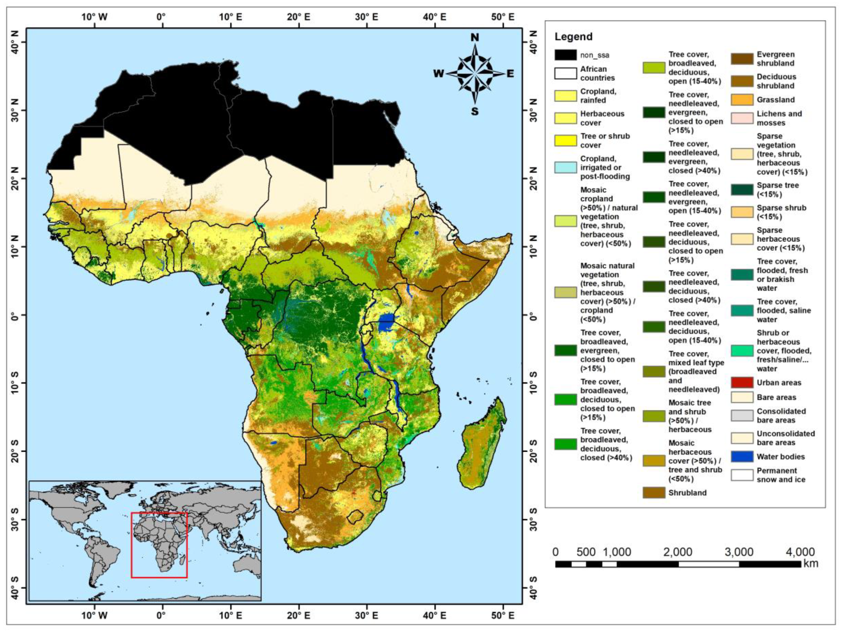
2. Study Area
3. Materials and Methods
3.1. Burned Area
3.2. Precipitation
3.3. Land Cover
3.4. Modern-Era Retrospective Analysis for Research and Applications Version 2 (MERRA-2)
3.5. CALIPSO (Cloud-Aerosol Lidar and Infrared Pathfinder Satellite Observations)
3.6. AIRS (Atmospheric Infrared Sounder)
3.7. Mann–Kendall Test
3.8. Sequential Mann–Kendall Test
4. Results
4.1. Seasonal Effects of Wildfires on Land Surface Dynamics
4.2. Seasonal Distribution of BC, CO and Smoke
4.3. The Effect of Meteorological Conditions on the Spatial and Seasonal Changes of Wildfires
4.4. Seasonal Trend Analysis over the Entire SSA Region
4.4.1. Linear Regression over the Entire Region
4.4.2. Mann–Kendall Trend Analysis over the Entire Region
4.4.3. Sequential Mann–Kendall Analysis over the Entire Region
4.5. Seasonal Trend Analysis over Northern and Southern Sub-regions of the SSA
5. Conclusions
Author Contributions
Funding
Acknowledgments
Conflicts of Interest
References
- Pio, C.; Legrand, M.; Alves, C.; Oliveira, T.S.; Afonso, J.; Caseiro, A.; Puxbaum, H.; Sanchez-Ochoa, A.; Gelencsér, A.; Pio, C.; et al. Chemical composition of atmospheric aerosols during the 2003 summer intense forest fire period. Atmos. Environ. 2008, 42, 7530–7543. [Google Scholar] [CrossRef]
- Chubarova, N.; Nezval, Y.; Sviridenkov, I.; Smirnov, A.; Slutsker, I. Smoke aerosol and its radiative effects during extreme fire event over Central Russia in summer 2010. Atmos. Meas. Tech. 2012, 5, 557–568. [Google Scholar] [CrossRef]
- Forkel, M.; Andela, N.; Harrison, S.P.; Lasslop, G.; Van Marle, M.; Chuvieco, E.; Dorigo, W.; Forrest, M.; Hantson, S.; Heil, A.; et al. Emergent relationships with respect to burned area in global satellite observations and fire-enabled vegetation models. Biogeosciences 2019, 16, 57–76. [Google Scholar] [CrossRef]
- Belward, A. The Global Observing System for Climate: Implementation Needs; World Meteorological Organization: Geneva, Switzerland, 2016; p. 315. [Google Scholar]
- Hitchcock, H.; Hoffer, R. Mapping a Recent Forest Fire with ERTS-1 MSS Data; NASA: Washington, DC, USA, 1974. [Google Scholar]
- Bastarrika, A.; Alvarado, M.; Artano, K.; Martínez, M.P.; Mesanza, A.; Torre, L.; Ramo, R.; Chuvieco, E. BAMS: A tool for supervised burned area mapping using Landsat data. Remote Sens. 2014, 6, 12360–12380. [Google Scholar] [CrossRef]
- Giglio, L.; Schroeder, W.; Justice, C.O. The collection 6 MODIS active fire detection algorithm and fire products. Remote. Sens. Environ. 2016, 178, 31–41. [Google Scholar] [CrossRef] [PubMed]
- Guindos-Rojas, F.; Arbelo, M.; García-Lázaro, J.R.; Moreno-Ruiz, J.A.; Hernandez-Leal, P.A. Evaluation of a Bayesian Algorithm to Detect Burned Areas in the Canary Islands’ Dry Woodlands and Forests Ecoregion Using MODIS Data. Remote Sens. 2018, 10, 789. [Google Scholar] [CrossRef]
- Long, T.; Zhang, Z.; He, G.; Jiao, W.; Tang, C.; Wu, B.; Zhang, X.; Wang, G.; Yin, R. 30 m Resolution Global Annual Burned Area Mapping Based on Landsat Images and Google Earth Engine. Remote. Sens. 2019, 11, 489. [Google Scholar] [CrossRef]
- Filipponi, F. Exploitation of Sentinel-2 Time Series to Map Burned Areas at the National Level: A Case Study on the 2017 Italy Wildfires. Remote. Sens. 2019, 11, 622. [Google Scholar] [CrossRef]
- Humber, M.L.; Boschetti, L.; Giglio, L.; Justice, C.O. Spatial and temporal intercomparison of four global burned area products. Int. J. Digit. Earth 2019, 12, 460–484. [Google Scholar] [CrossRef]
- Cardozo, F.d.S.; Shimabukuro, Y.E.; Pereira, G.; Silva, F.B. Using remote sensing products for environmental analysis in South America. Remote Sens. 2011, 3, 2110–2127. [Google Scholar] [CrossRef]
- De Sales, F.; Xue, Y.; Okin, G.S. Impact of burned areas on the northern African seasonal climate from the perspective of regional modeling. Clim. Dyn. 2016, 47, 3393–3413. [Google Scholar] [CrossRef]
- De Sales, F.; Okin, G.S.; Xue, Y.; Dintwe, K. On the effects of wildfires on precipitation in Southern Africa. Clim. Dyn. 2019, 52, 951–967. [Google Scholar] [CrossRef]
- Randerson, J.T.; Chen, Y.; Van Der Werf, G.R.; Rogers, B.M.; Morton, D.C. Global burned area and biomass burning emissions from small fires. J. Geophys. Res. Biogeosci. 2012, 117. [Google Scholar] [CrossRef]
- Giglio, L.; Randerson, J.T.; Van Der Werf, G.R. Analysis of daily, monthly, and annual burned area using the fourth-generation global fire emissions database (GFED4). J. Geophys. Res. Biogeosci. 2013, 118, 317–328. [Google Scholar] [CrossRef]
- Zielinski, T.; Petelski, T.; Strzalkowska, A.; Pakszys, P.; Makuch, P. Impact of wild forest fires in Eastern Europe on aerosol composition and particle optical properties. Oceanologia 2016, 58, 13–24. [Google Scholar] [CrossRef]
- Ito, A.; Penner, J.E. Historical emissions of carbonaceous aerosols from biomass and fossil fuel burning for the period 1870–2000. Glob. Biogeochem. Cycles 2005, 19. [Google Scholar] [CrossRef]
- Langmann, B.; Duncan, B.; Textor, C.; Trentmann, J.; van der Werf, G.R. Vegetation fire emissions and their impact on air pollution and climate. Atmos. Environ. 2009, 43, 107–116. [Google Scholar] [CrossRef]
- Andreae, M.; Rosenfeld, D.; Artaxo, P.; Costa, A.A.; Frank, G.P.; Longo, K.M.; Silva-Dias, M.A.F. Smoking rain clouds over the Amazon. Science 2004, 303, 1337–1342. [Google Scholar] [CrossRef]
- Johnston, F.H.; Henderson, S.B.; Chen, Y.; Randerson, J.T.; Marlier, M.; DeFries, R.S.; Kinney, P.; Bowman, D.M.; Brauer, M. Estimated global mortality attributable to smoke from landscape fires. Environ. Health Perspect. 2012, 120, 695–701. [Google Scholar] [CrossRef]
- Shrestha, G.; Traina, S.J.; Swanston, C.W. Black Carbon’s Properties and Role in the Environment: A Comprehensive Review. Sustainability 2010, 2, 294–320. [Google Scholar] [CrossRef]
- Jian, Y.; Fu, T.-M. Injection heights of springtime biomass-burning plumes over peninsular Southeast Asia and their impacts on long-range pollutant transport. Atmos. Chem. Phys. 2014, 14, 3977–3989. [Google Scholar] [CrossRef]
- Zhu, L.; Val Martin, M.; Hecobian, A.; Gatti, L.; Kahn, R.; Fischer, E. Development and implementation of a new biomass burning emissions injection height scheme for the GEOS-Chem model. Geosci. Model Dev. 2018, 2018, 1–30. [Google Scholar]
- Martin, M.V.; Kahn, R.A.; Tosca, M.G. A Global Analysis of Wildfire Smoke Injection Heights Derived from Space-Based Multi-Angle Imaging. Remote Sens. 2018, 10, 1609. [Google Scholar] [CrossRef]
- Ditas, J.; Ma, N.; Zhang, Y.; Assmann, D.; Neumaier, M.; Riede, H.; Karu, E.; Williams, J.; Scharffe, D.; Wang, Q.; et al. Strong impact of wildfires on the abundance and aging of black carbon in the lowermost stratosphere. Proc. Natl. Acad. Sci. USA 2018, 115, E11595–E11603. [Google Scholar] [CrossRef] [PubMed]
- Wang, W.; Liang, S.; Meyers, T. Validating MODIS land surface temperature products using long-term nighttime ground measurements. Remote Sens. Environ. 2008, 112, 623–635. [Google Scholar] [CrossRef]
- Bond, T.C.; Doherty, S.J.; Fahey, D.W.; Forster, P.M.; Berntsen, T.; DeAngelo, B.J.; Flanner, M.G.; Ghan, S.; Kärcher, B.; Koch, D.; et al. Bounding the role of black carbon in the climate system: A scientific assessment. J. Geophys. Res. Atmos. 2013, 118, 5380–5552. [Google Scholar] [CrossRef]
- Sims, R.; Gorsevski, V.; Anenberg, S. Black Carbon Mitigation and the Role of the Global Environment Facility: A STAP Advisory Document; United Nations Environment Programme: Nairobi, Kenya, 2015. [Google Scholar]
- Woodcock, J.; Edwards, P.; Tonne, C.; Armstrong, B.G.; Ashiru, O.; Banister, D.; Beevers, S.; Chalabi, Z.; Chowdhury, Z.; Cohen, A.; et al. Public health benefits of strategies to reduce greenhouse-gas emissions: Urban land transport. Lancet 2009, 374, 1930–1943. [Google Scholar] [CrossRef]
- Ruiz-Mercado, I.; Masera, O.; Zamora, H.; Smith, K.R. Adoption and sustained use of improved cookstoves. Energy Policy 2011, 39, 7557–7566. [Google Scholar] [CrossRef]
- Shikwambana, L.; Sivakumar, V. Global distribution of aerosol optical depth in 2015 using CALIPSO level 3 data. J. Atmos. Sol. Terr. Phys. 2018, 173, 150–159. [Google Scholar] [CrossRef]
- Shikwambana, L. Long-term observation of global black carbon, organic carbon and smoke using CALIPSO and MERRA-2 data. Remote Sens. Lett. 2019, 10, 373–380. [Google Scholar] [CrossRef]
- Lasko, K.; Vadrevu, K.P.; Nguyen, T.T.N. Analysis of air pollution over Hanoi, Vietnam using multi-satellite and MERRA reanalysis datasets. PLoS ONE 2018, 13, e0196629. [Google Scholar] [CrossRef] [PubMed]
- Olson, D.M.; Dinerstein, E.; Wikramanayake, E.D.; Burgess, N.D.; Powell, G.V.; Underwood, E.C.; D’amico, J.A.; Itoua, I.; Strand, H.E.; Morrison, J.C. Terrestrial Ecoregions of the World: A New Map of Life on EarthA new global map of terrestrial ecoregions provides an innovative tool for conserving biodiversity. BioScience 2001, 51, 933–938. [Google Scholar] [CrossRef]
- Giglio, L.; Justice, C.; Boschetti, L.; Roy, D. MCD64A1 MODIS/Terra+ Aqua Burned Area Monthly L3 Global 500 m SIN Grid V006 [Data Set]; NASA EOSDIS Land Processes DAAC: Sioux Falls, SD, USA, 2015. [Google Scholar]
- Giglio, L.; Boschetti, L.; Roy, D.P.; Humber, M.L.; Justice, C.O. The Collection 6 MODIS burned area mapping algorithm and product. Remote Sens. Environ. 2018, 217, 72–85. [Google Scholar] [CrossRef] [PubMed]
- Defourny, P.; Brockmann, C.; Bontemps, S.; Lamarche, C.; Santoro, M.; Boettcher, M.; Wevers, J. CCI-LC PUGv2 Phase II. Land Cover Climate Change Initiative-Product User Guide v2. 2017. Available online: https://www.esa-landcover-cci.org/?q=webfm_send/84 (accessed on 4 August 2019).
- Li, W.; MacBean, N.; Ciais, P.; Defourny, P.; Lamarche, C.; Bontemps, S.; Houghton, R.A.; Peng, S. Gross and net land cover changes in the main plant functional types derived from the annual ESA CCI land cover maps (1992–2015). Earth Syst. Sci. Data 2018, 10, 219–234. [Google Scholar] [CrossRef] [Green Version]
- Bontemps, S.; Defourny, P.; Radoux, J.; Van Bogaert, E.; Lamarche, C.; Achard, F.; Mayaux, P.; Boettcher, M.; Brockmann, C.; Kirches, G. Consistent global land cover maps for climate modelling communities: Current achievements of the ESA’s land cover CCI. In Proceedings of the ESA Living Planet Symposium, Edimburgh, UK, 9–13 September 2013; pp. 9–13. [Google Scholar]
- Rienecker, M.M.; Suarez, M.J.; Gelaro, R.; Todling, R.; Bacmeister, J.; Liu, E.; Bosilovich, M.G.; Schubert, S.D.; Takacs, L.; Kim, G.-K.; et al. MERRA: NASA’s modern-era retrospective analysis for research and applications. J. Clim. 2011, 24, 3624–3648. [Google Scholar] [CrossRef]
- Buchard, V.; Da Silva, A.M.; Colarco, P.R.; Darmenov, A.; Randles, C.A.; Govindaraju, R.; Torres, O.; Campbell, J.; Spurr, R. Using the OMI aerosol index and absorption aerosol optical depth to evaluate the NASA MERRA Aerosol Reanalysis. Atmos. Chem. Phys. 2015, 15, 5743. [Google Scholar] [CrossRef] [Green Version]
- Buchard, V.; da Silva, A.; Randles, C.; Colarco, P.; Ferrare, R.; Hair, J.; Hostetler, C.; Tackett, J.; Winker, D. Evaluation of the surface PM2.5 in Version 1 of the NASA MERRA Aerosol Reanalysis over the United States. Atmos. Environ. 2016, 125, 100–111. [Google Scholar] [CrossRef]
- Stephens, G.L.; Vane, D.G.; Boain, R.J.; Mace, G.G.; Sassen, K.; Wang, Z.; Illingworth, A.J.; O’connor, E.J.; Rossow, W.B.; Durden, S.L. The CloudSat mission and the A-Train: A new dimension of space-based observations of clouds and precipitation. Bull. Am. Meteorol. Soc. 2002, 83, 1771–1790. [Google Scholar] [CrossRef] [Green Version]
- Hunt, W.H.; Winker, D.M.; Vaughan, M.A.; Powell, K.A.; Lucker, P.L.; Weimer, C. CALIPSO lidar description and performance assessment. J. Atmos. Ocean. Technol. 2009, 26, 1214–1228. [Google Scholar] [CrossRef]
- Winker, D.M.; Pelon, J.R.; McCormick, M.P. The CALIPSO mission: Spaceborne lidar for observation of aerosols and clouds. In Lidar Remote Sensing for Industry and Environment Monitoring III; Society of Photo Optical: Bellingham, WA, USA, 2002; pp. 1–12. [Google Scholar]
- Winker, D.; Pelon, J.; Coakley, J.A., Jr.; Ackerman, S.; Charlson, R.; Colarco, P.; Flamant, P.; Fu, Q.; Hoff, R.; Kittaka, C. The CALIPSO mission: A global 3D view of aerosols and clouds. Bull. Am. Meteorol. Soc. 2010, 91, 1211–1230. [Google Scholar] [CrossRef]
- Aumann, H.; Chahine, M.; Gautier, C.; Goldberg, M.; Kalnay, E.; McMillin, L.; Revercomb, H.; Rosenkranz, P.; Smith, W.; Staelin, D.; et al. AIRS/AMSU/HSB on the Aqua mission: Design, science objectives, data products, and processing systems. IEEE Trans. Geosci. Remote Sens. 2003, 41, 253–264. [Google Scholar] [CrossRef] [Green Version]
- Tobin, D.C.; Revercomb, H.E.; Knuteson, R.O.; Lesht, B.M.; Strow, L.L.; Hannon, S.E.; Feltz, W.F.; Moy, L.A.; Fetzer, E.J.; Cress, T.S. Atmospheric Radiation Measurement site atmospheric state best estimates for Atmospheric Infrared Sounder temperature and water vapor retrieval validation. J. Geophys. Res. Atmos. 2006, 111. [Google Scholar] [CrossRef] [Green Version]
- Mann, H.B. Nonparametric tests against trend. Econom. J. Econom. Soc. 1945, 13, 245–259. [Google Scholar] [CrossRef]
- Kendall, M.G. Rank Correlation Methods; The Griffin: London, UK, 1948. [Google Scholar]
- Pal, I.; Al-Tabbaa, A. Trends in seasonal precipitation extremes—An indicator of ‘climate change’ in Kerala, India. J. Hydrol. 2009, 367, 62–69. [Google Scholar] [CrossRef]
- Sneyers, R. On the Statistical Analysis of Series of Observations; World Meteorological Organization (WMO): Geneva, Switzerland, 1991. [Google Scholar]
- Mosmann, V.; Castro, A.; Fraile, R.; Dessens, J.; Sanchez, J.L. Detection of statistically significant trends in the summer precipitation of mainland Spain. Atmos. Res. 2004, 70, 43–53. [Google Scholar] [CrossRef]
- Adarsh, S.; Janga Reddy, M. Trend analysis of rainfall in four meteorological subdivisions of southern India using nonparametric methods and discrete wavelet transforms. Int. J. Climatol. 2015, 35, 1107–1124. [Google Scholar] [CrossRef]
- Verhegghen, A.; Eva, H.; Ceccherini, G.; Achard, F.; Gond, V.; Gourlet-Fleury, S.; Cerutti, P.O. The potential of Sentinel satellites for burnt area mapping and monitoring in the Congo Basin forests. Remote Sens. 2016, 8, 986. [Google Scholar] [CrossRef] [Green Version]
- Koutsias, N.; Xanthopoulos, G.; Founda, D.; Xystrakis, F.; Nioti, F.; Pleniou, M.; Mallinis, G.; Arianoutsou, M. On the relationships between forest fires and weather conditions in Greece from long-term national observations (1894–2010). Int. J. Wildland Fire 2013, 22, 493–507. [Google Scholar] [CrossRef] [Green Version]
- Bedia, J.; Herrera, S.; Gutiérrez, J.M.; García, S.H. Assessing the predictability of fire occurrence and area burned across phytoclimatic regions in Spain. Nat. Hazards Earth Syst. Sci. 2014, 14, 53–66. [Google Scholar] [CrossRef] [Green Version]
- Barlow, J.; Peres, C.A.; Lagan, B.O.; Haugaasen, T. Large tree mortality and the decline of forest biomass following Amazonian wildfires. Ecol. Lett. 2003, 6, 6–8. [Google Scholar] [CrossRef]
- Varma, A. The economics of slash and burn: A case study of the 1997–1998 Indonesian forest fires. Ecol. Econ. 2003, 46, 159–171. [Google Scholar] [CrossRef]
- Cochrane, M.A. Fire science for rainforests. Nature 2003, 421, 913. [Google Scholar] [CrossRef] [PubMed]
- Uhl, C.; Kauffman, J.B. Deforestation, fire susceptibility, and potential tree responses to fire in the eastern Amazon. Ecology 1990, 71, 437–449. [Google Scholar] [CrossRef]
- Trollope, W. Role of fire in preventing bush encroachment in the Eastern Cape. Proc. Annu. Congr. Grassl. Soc. South. Afr. 1974, 9, 67–72. [Google Scholar] [CrossRef]
- Snyman, H. Short-term response of the encroacher shrub Seriphium plumosum to fire. Afr. J. Range Forage Sci. 2011, 28, 65–77. [Google Scholar] [CrossRef]
- Snyman, H. Estimating the short-term impact of fire on rangeland productivity in a semi-arid climate of South Africa. J. Arid Environ. 2004, 59, 685–697. [Google Scholar] [CrossRef]
- Snyman, H. Short-term response in productivity following an unplanned fire in a semi-arid rangeland of South Africa. J. Arid Environ. 2004, 56, 465–485. [Google Scholar] [CrossRef]
- Everson, C.S.; Everson, T. The long-term effects of fire regime on primary production of montane grasslands in South Africa. Afr. J. Range Forage Sci. 2016, 33, 33–41. [Google Scholar] [CrossRef]
- Breedt, J.A.; Dreber, N.; Kellner, K. Post-wildfire regeneration of rangeland productivity and functionality—Observations across three semi-arid vegetation types in South Africa. Afr. J. Range Forage Sci. 2013, 30, 161–167. [Google Scholar] [CrossRef]
- Snyman, H. Short-term response of burnt grassland to defoliation in a semi-arid climate of South Africa. Afr. J. Range Forage Sci. 2006, 23, 1–11. [Google Scholar] [CrossRef]
- La Rosa, N.S.-D.; González-Cardoso, G.; Figueroa-Lara, J.D.J.; Gutiérrez-Arzaluz, M.; Octaviano-Villasana, C.; Ramírez-Hernández, I.F.; Mugica-Álvarez, V. Emission factors of atmospheric and climatic pollutants from crop residues burning. J. Air Waste Manag. Assoc. 2018, 68, 849–865. [Google Scholar] [CrossRef] [PubMed] [Green Version]
- Adeyolanu, O.D.; Are, K.S.; Oluwatosin, G.A.; Ayoola, O.T.; Adelana, A.O. Evaluation of two methods of soil quality assessment as influenced by slash and burn in tropical rainforest ecology of Nigeria. Arch. Agron. Soil Sci. 2013, 59, 1725–1742. [Google Scholar] [CrossRef]
- Liousse, C.; Guillaume, B.; Grégoire, J.M.; Mallet, M.; Galy, C.; Pont, V.; Akpo, A.; Bedou, M.; Castera, P.; Dungall, L.; et al. Updated African biomass burning emission inventories in the framework of the AMMA-IDAF program, with an evaluation of combustion aerosols. Atmos. Chem. Phys. 2010, 10, 9631–9646. [Google Scholar] [CrossRef] [Green Version]
- Suman, D. Biomass burning in North Africa and its possible relationship to climate change in the mediterranean basin. In The Impact of Desert Dust Across the Mediterranean; Springer: Berlin, Germany, 1996; pp. 113–122. [Google Scholar]
- Reid, J.; Koppmann, R.; Eck, T.; Eleuterio, D. A review of biomass burning emissions part II: Intensive physical properties of biomass burning particles. Atmos. Chem. Phys. 2005, 5, 799–825. [Google Scholar] [CrossRef] [Green Version]
- Carslaw, K.; Boucher, O.; Spracklen, D.; Mann, G.; Rae, J.; Woodward, S.; Kulmala, M. A review of natural aerosol interactions and feedbacks within the Earth system. Atmos. Chem. Phys. 2010, 10, 1701–1737. [Google Scholar] [CrossRef] [Green Version]
- Zheng, X.; Zhang, S.; Wu, Y.; Zhang, K.M.; Wu, X.; Li, Z.; Hao, J. Characteristics of black carbon emissions from in-use light-duty passenger vehicles. Environ. Pollut. 2017, 231, 348–356. [Google Scholar] [CrossRef]
- Efe, S. Spatial distribution of particulate air pollution in Nigerian cities: Implications for human health. J. Environ. Health Res. 2008, 7, 107–116. [Google Scholar]
- Wang, R.; Balkanski, Y.; Boucher, O.; Ciais, P.; Schuster, G.L.; Chevallier, F.; Samset, B.H.; Liu, J.; Piao, S.; Valari, M.; et al. Estimation of global black carbon direct radiative forcing and its uncertainty constrained by observations. J. Geophys. Res. Atmos. 2016, 121, 5948–5971. [Google Scholar] [CrossRef]
- Löndahl, J.; Swietlicki, E.; Pagels, J.; Massling, A.; Boman, C.; Rissler, J.; Blomberg, A.; Sandström, T. Respiratory tract deposition of particles from biomass combustion. J. Phys. Conf. Ser. 2009, 151, 012066. [Google Scholar] [CrossRef]
- Lin, N.-H.; Tsay, S.-C.; Maring, H.B.; Yen, M.-C.; Sheu, G.-R.; Wang, S.-H.; Chi, K.H.; Chuang, M.-T.; Ou-Yang, C.-F.; Fu, J.S.; et al. An overview of regional experiments on biomass burning aerosols and related pollutants in Southeast Asia: From BASE-ASIA and the Dongsha Experiment to 7-SEAS. Atmos. Environ. 2013, 78, 1–19. [Google Scholar] [CrossRef] [Green Version]
- Dwyer, E.; Pinnock, S.; Grégoire, J.-M.; Pereira, J. Global spatial and temporal distribution of vegetation fire as determined from satellite observations. Int. J. Remote Sens. 2000, 21, 1289–1302. [Google Scholar] [CrossRef]
- Suzuki, M.; Kushida, H.; Dobashi, R.; Hirano, T. Effects of humidity and temperature on downward flame spread over filter paper. Fire Saf. Sci. 2000, 6, 661–669. [Google Scholar] [CrossRef]
- Li, F.; Lawrence, D.M.; Bond-Lamberty, B. Impact of fire on global land surface air temperature and energy budget for the 20th century due to changes within ecosystems. Environ. Res. Lett. 2017, 12, 044014. [Google Scholar] [CrossRef]
- Turco, M.; Levin, N.; Tessler, N.; Saaroni, H. Recent changes and relations among drought, vegetation and wildfires in the Eastern Mediterranean: The case of Israel. Glob. Planet. Chang. 2017, 151, 28–35. [Google Scholar] [CrossRef]
- Kutiel, H. Weather conditions and forest fire propagation—The case of the carmel fire, December 2010. Isr. J. Ecol. Evol. 2012, 58, 113–122. [Google Scholar]
- Mehta, M.; Singh, R.; Singh, A.; Singh, N. Recent global aerosol optical depth variations and trends—A comparative study using MODIS and MISR level 3 datasets. Remote Sens. Environ. 2016, 181, 137–150. [Google Scholar] [CrossRef]
- Roberts, G.; Wooster, M.; Lagoudakis, E. Annual and diurnal african biomass burning temporal dynamics. Biogeosciences 2009, 6, 849–866. [Google Scholar] [CrossRef] [Green Version]
- Cowie, S.M.; Knippertz, P.; Marsham, J.H. Are vegetation-related roughness changes the cause of the recent decrease in dust emission from the Sahel? Geophys. Res. Lett. 2013, 40, 1868–1872. [Google Scholar] [CrossRef] [Green Version]
- Dardel, C.; Kergoat, L.; Hiernaux, P.; Mougin, E.; Grippa, M.; Tucker, C. Re-greening Sahel: 30 years of remote sensing data and field observations (Mali, Niger). Remote Sens. Environ. 2014, 140, 350–364. [Google Scholar] [CrossRef]
- Olsson, L.; Eklundh, L.; Ardö, J. A recent greening of the Sahel—Trends, patterns and potential causes. J. Arid Environ. 2005, 63, 556–566. [Google Scholar] [CrossRef]
- Collins, J.M. Temperature variability over Africa. J. Clim. 2011, 24, 3649–3666. [Google Scholar] [CrossRef] [Green Version]
- Serdeczny, O.; Adams, S.; Baarsch, F.; Coumou, D.; Robinson, A.; Hare, W.; Schaeffer, M.; Perrette, M.; Reinhardt, J. Climate change impacts in Sub-Saharan Africa: From physical changes to their social repercussions. Reg. Environ. Chang. 2017, 17, 1585–1600. [Google Scholar] [CrossRef]
- Ritchie, H.; Roser, M. CO2 and Greenhouse Gas Emissions. Our World Data, 2017. Available online: https://ourworlddata.org/co2-and-other-greenhouse-gas-emissions (accessed on 13 November 2019).
- Kumar, K.R.; Sivakumar, V.; Yin, Y.; Reddy, R.; Kang, N.; Diao, Y.; Adesina, A.J.; Yu, X. Long-term (2003–2013) climatological trends and variations in aerosol optical parameters retrieved from MODIS over three stations in South Africa. Atmos. Environ. 2014, 95, 400–408. [Google Scholar] [CrossRef]
- Kelly, L.; Brotons, L. Using fire to promote biodiversity. Science 2017, 355, 1264–1265. [Google Scholar] [CrossRef] [PubMed]
- Jeong, G.-R.; Wang, C. Climate effects of seasonally varying Biomass Burning emitted Carbonaceous Aerosols (BBCA). Atmos. Chem. Phys. 2010, 10, 8373–8389. [Google Scholar] [CrossRef] [Green Version]
- Giglio, L.; Csiszar, I.; Justice, C.O. Global distribution and seasonality of active fires as observed with the Terra and Aqua Moderate Resolution Imaging Spectroradiometer (MODIS) sensors. J. Geophys. Res. Biogeosci. 2006, 111. [Google Scholar] [CrossRef]
- Mao, K.; Ma, Y.; Xia, L.; Chen, W.Y.; Shen, X.; He, T.; Xu, T. Global aerosol change in the last decade: An analysis based on MODIS data. Atmos. Environ. 2014, 94, 680–686. [Google Scholar] [CrossRef] [Green Version]


| Parameter | p-Value | H0 |
|---|---|---|
| BC | 0.0518 | Failed, No Significant Trend |
| CO | 0.0366 | Rejected, Significant Trend |
| Latent Heat Flux | 1.65 × 10⁻⁹ | Rejected, Significant Trend |
| Precipitation | 0.0308 | Rejected, Significant Trend |
| Relative Surface Humidity | 0.440 | Failed, No Significant Trend |
| Burn area | 0.754 | Failed, No Significant Trend |
| Parameter | DJF | MAM | JJA | SON |
|---|---|---|---|---|
| p-Value | p-Value | p-Value | p-Value | |
| BC | 0.1096 | 0.0074 * | 0.0124 * | 0.9870 |
| CO | 0.7330 | 0.0028 * | 1.202 × 10⁻⁴ * | 0.9224 |
| Latent Heat Flux | 0.0047 * | 7.720 × 10⁻⁴ * | 1.402 × 10⁻⁶ * | 6.09 × 10⁻⁴ * |
| Precipitation | 0.0230 * | 0.3379 | 0.3461 | 0.3630 |
| Relative Surface Humidity | 0.7220 | 0.1292 | 0.8965 | 0.8679 |
| Burn area | 0.2984 | 0.0831 | 3.798 × 10⁻⁹ * | 3.906 × 10⁻⁴ * |
| Parameter | Northern SSA | Southern SSA |
|---|---|---|
| p-Value | p-Value | |
| BC | 0.05 | 0.08 |
| Latent Heat Flux | 6.0797 × 10⁻⁶ | 0.39 |
| Relative Surface Humidity | 0.51 | 0.80 |
© 2019 by the authors. Licensee MDPI, Basel, Switzerland. This article is an open access article distributed under the terms and conditions of the Creative Commons Attribution (CC BY) license (http://creativecommons.org/licenses/by/4.0/).
Share and Cite
Kganyago, M.; Shikwambana, L. Assessing Spatio-Temporal Variability of Wildfires and their Impact on Sub-Saharan Ecosystems and Air Quality Using Multisource Remotely Sensed Data and Trend Analysis. Sustainability 2019, 11, 6811. https://doi.org/10.3390/su11236811
Kganyago M, Shikwambana L. Assessing Spatio-Temporal Variability of Wildfires and their Impact on Sub-Saharan Ecosystems and Air Quality Using Multisource Remotely Sensed Data and Trend Analysis. Sustainability. 2019; 11(23):6811. https://doi.org/10.3390/su11236811
Chicago/Turabian StyleKganyago, Mahlatse, and Lerato Shikwambana. 2019. "Assessing Spatio-Temporal Variability of Wildfires and their Impact on Sub-Saharan Ecosystems and Air Quality Using Multisource Remotely Sensed Data and Trend Analysis" Sustainability 11, no. 23: 6811. https://doi.org/10.3390/su11236811