1. Introduction
In this paper, we consider a two-machine flowshop scheduling problem where the processing times are linearly dependent on the waiting times of the jobs prior to processing on the second machine. The objective is to minimize the makespan. In this problem, when a job is processed completely on the first machine, a certain delay time is required before its processing on the second machine. If we can find a way to reduce the certain delay time at the cost of extra processing time added to the processing time of the job on the second machine, the whole processing time of all jobs may be reduced. When the whole processing time is reduced, the consumption of energy is reduced. This contributes to environmental sustainability. In addition, the managerial implication of this approach is that a production scheduler has more leeway to arrange a job sequence to reach the goal. One realistic example of this kind of scheduling exists in a painting process. Generally, there are at least two layer-painting stages in a painting engineering. After the first stage, the product has to wait for some time until it is dry naturally. Then, the product goes to the second stage. If we want to reduce the waiting time, we can use a dryer to accelerate the drying process. This implies that the cost of extra processing time is added to the processing time of the job on the second machine. Another practical scheduling problem arises at the cooking–chilling stage in a food plant [
1]. The chilling process must start within 30 min of the completion of cooking. Otherwise, the food has to be discarded as unfit for human consumption. If there is an advantage in terms of the makespan minimization, we can reduce the waiting time after the completion of cooking at the cost of an extra processing time of the chilling process. In such a situation, it is good for the sustainability of the earth because it involves less food waste. Also, the objective of the makespan is minimized. The processing time of all jobs is reduced. The consumption of the energy is reduced. It is beneficial for environmental sustainability. For some other scheduling problems related to sustainability, the reader is referred to the works of [
2,
3,
4,
5,
6,
7,
8].
The two-machine, minimum makespan, flowshop scheduling problem was first solved by Johnson [
9]. Mitten [
10] extended this problem with time lags. Sule and Huang [
11] permitted the setup and removal times to be independent of the processing time. Maggu et al. [
12] considered the problem with time lags and transportation time between machines. These problems proposed above are solved by a polynomial time algorithm, which is similar to Johnson’s rule [
9]. There are also many studies considering scheduling problems with sequence dependent setup time. For example, Ruiz [
13] proposed an iterated greedy heuristic to solve the flowshop scheduling problem with sequence dependent setup time. Nishi and Hiranaka [
14] applied the Lagrangian relaxation and cut generation method to minimize the total weighted tardiness in flowshop scheduling problems with sequence dependent setup time. Wang et al. [
15] presented a hybrid local search algorithm to solve the sequence setup times flowshop scheduling problem with a makespan criterion.
For the two-machine flowshop scheduling problem with waiting time constraints (or intermediate delays), Reddi and Ramamoorthy [
16] proposed a polynomial time algorithm for the problem with no-wait in process. Dell’Amico [
17] showed that the two-machine flowshop scheduling problem with intermediate delays is NP-hard in the strong sense if the solution space is not restricted to permutation schedules. In addition, Yu et al. [
18] showed that the two-machine flowshop machine problem with intermediate delays is NP-hard in the strong sense, even if all processing times are 1. Fiszmann and Mosheiov [
19] studied the scheduling problem of minimizing total load on a proportionate flowshop. They considered position-dependent job processing times in the most general way. They showed that this problem is solved in O(
) time, where
n is the number of jobs. Yang and Chern [
20] considered a two-machine flowshop sequencing problem with limited waiting time constraints; they showed that the permutation scheduling problem is NP-hard and proposed a branch-and-bound algorithm. Su [
21] extended the problem studied by Yang and Chern [
20] and considered a two-stage flowshop with a batch processor in stage 1 and a single processor in stage 2. Each batch processor can process a batch (limited number) of jobs simultaneously. A heuristic algorithm and a mixed integer program are proposed. Sriskandarajah and Goyal [
22] considered a problem in which the processing times are linearly dependent on the waiting times; they showed that the problem is NP-hard and proposed a heuristic algorithm. Yang and Chern [
23] further extended the problem studied by Sriskandarajah and Goyal [
22] and considered a problem in which the processing time of a job on the second machine is linearly dependent on the waiting time if the waiting time is beyond a certain range. They proposed an integer program and a heuristic algorithm to solve the problem.
Chung et al. [
24] considered a two-stage hybrid flowshop scheduling problem with a waiting time constraint. They provided two algorithms to solve the makespan minimization problem. Wang et al. [
25] investigated a permutation flowshop scheduling problem with a time lag between two consecutive machines. They presented a two-stage constructive heuristic to minimize the makespan.
The proposed problem is different from those studied by Sriskandarajah and Goyal [
22] and Yang and Chern [
23]. In the problem of Sriskandarajah and Goyal [
22], when a job is processed completely on the first machine, the job can be processed immediately on the second machine. No delay time is required. If there is a delay time before a job to be processed on the second machine, the processing time of the job on the second machine increases. In the problem of Yang and Chern [
23], when a job is processed completely on the first machine, there is a waiting time before its processing on the second machine. If the waiting time is beyond a certain range, the processing time of a job on the second machine increases. This problem is similar to the following problem. When a job is processed completely on the first machine, a certain delay time (i.e., a certain waiting time) is required before its processing on the second machine. However, the
actual waiting time can be either decreased or increased. The cost of the actual waiting time change is the increase of the processing time of a job on the second machine. In the proposed problem, we only consider the case in which the actual waiting time is allowed to be decreased at the cost of extra processing time added to the processing time of a job on the second machine.
The organization of the remainder of this paper is as follows. In
Section 2, there is a description of the problem and its complexity. A 0-1 mixed integer programming formulation is given in
Section 3 and the heuristic algorithm is presented in
Section 4. Thereafter, computational experiments are reported in
Section 5. Finally, in
Section 6, we give the conclusions.
2. Problem Description and Complexity
The proposed two-machine makespan flowshop scheduling problem denoted T with processing time linearly dependent on job waiting time is described as follows.
First, some notations are introduced in the following and additional notations will be given when needed throughout the paper.
Ji: the ith job in the original sequence, i = 1, 2, 3,…, n
J[i]: the ith job in the actual sequence, i = 1, 2, 3,…, n
M1: the first machine on the flowshop
M2: the second machine on the flowshop
ai: the regular processing time of Ji on the first machine M1
bi: the regular processing time of Ji on the second machine M2
di: the delay time of Ji before its processing on machine M2
wi: the actual waiting time of Ji before its processing on machine M2
αi: the cost index, αi > 0
Ci,1: the completion time of Ji on machine M1
Ci,2: the completion time of Ji on machine M2
For a given set of jobs J = {J1, J2, …, Jn}, let ai and bi be the regular processing times of job Ji on the first machine M1 and the second machine M2, respectively. We assume that for each job Ji, when Ji is processed completely on machine M1, a delay time di is required before its processing on machine M2. However, in some situations, the actual waiting time wi is allowed to be smaller than the delay time di at the cost of extra processing time added to the processing time bi of job Ji on M2. That is, if the actual waiting time wi of Ji is smaller than di, then the processing time of Ji on machine M2 is given by bi + αi(di − wi), where αi > 0. However, if wi ≥ di, then the processing time on machine M2 is bi. The objective is to find the optimal schedule minimizing the makespan.
First, in the proposed problem, if
, there is no benefit to reduce the actual time
wi, and then the proposed problem is reduced to the problem studied in Yu et al. [
18]. Hence, if
, the proposed problem is also NP-hard in the strong sense. Next, we will show that the partition problem [
26] reduces to the proposed problem if
,
i = 1, …,
n. Consider the following well-known NP-complete problem:
Partition: Given positive integers
s1,
s2, …,
sk, does there exist a subset
For a given instance of partition,
s1,
s2, …,
sk, an instance of the proposed problem is constructed as follows:
where
= 2
S.
We will show that Partition has a solution if and only if the above instance has an optimal schedule with the minimum makespan Cmax = 4S2 + S + 3.
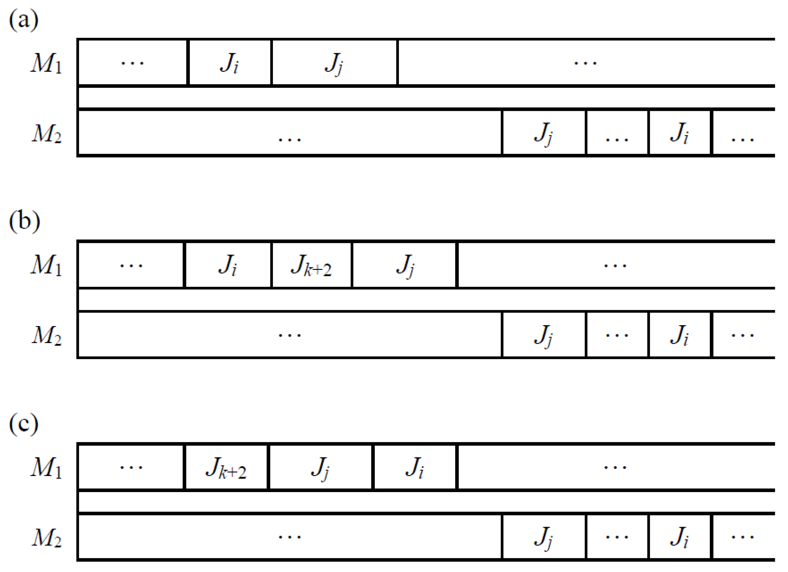
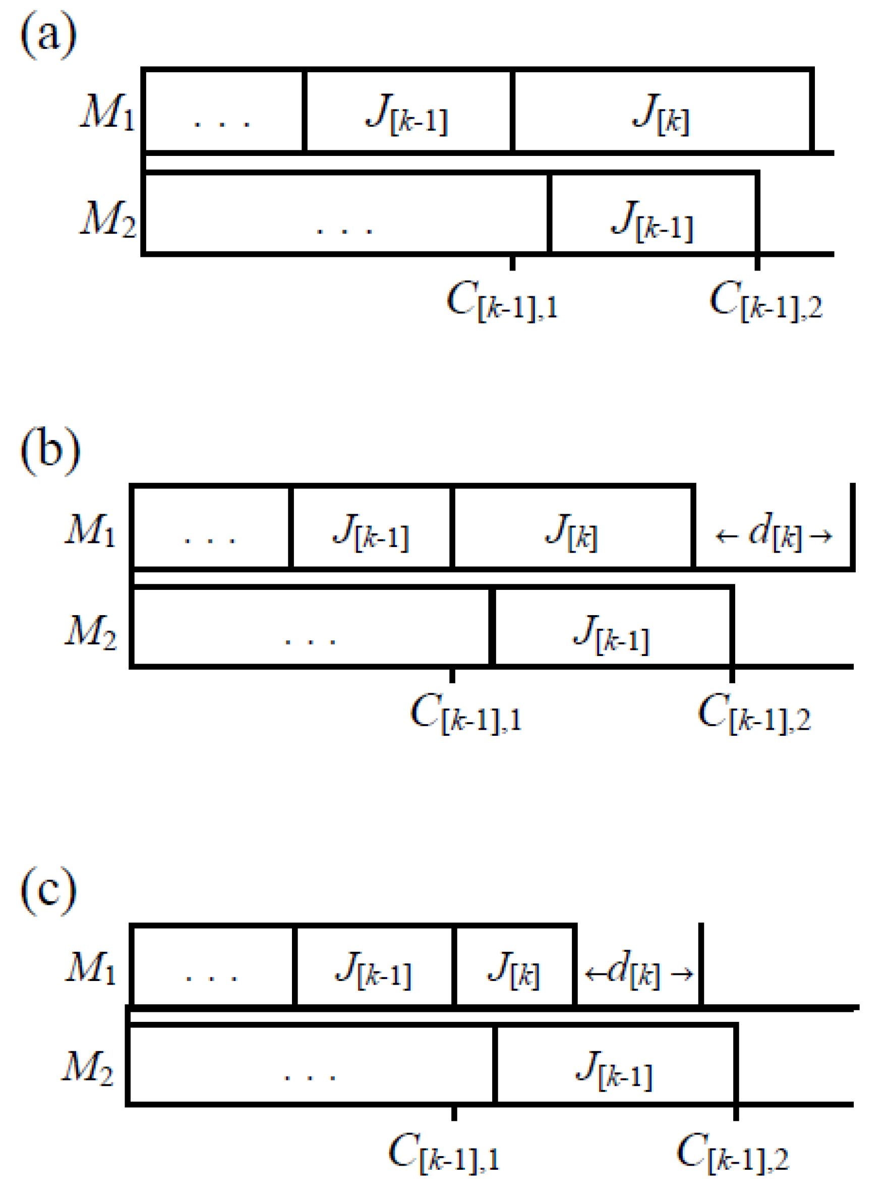
Lemma 1. For the above instance, it is sufficient to consider the schedules that have the same job processing sequence on both machines for the job Ji, i ∈ {1, …, k + 1}.
Proof. If a schedule Π does not have the same job processing sequence on both machines for the job Ji, i∈{1, …, k + 1}, then there are two cases:
- (1)
There is a job
Ji, which directly precedes
Jj on machine
M1 and follows
Jj on machine
M2,
i,
j ∈ {1, …,
k + 1}, perhaps with intervening jobs (
Figure 1a). We may interchange the order of
Ji and
Jj on machine
M1 without increasing the makespan, because
di =
dj = 0.
- (2)
There is a sequence (
A1,
Ji,
Jk+2,
Jj, A2) on machine
M1, where
A1 and
A2 are subsequences, and
Ji follows
Jj on machine
M2, perhaps with intervening jobs (
Figure 1b). We may interchange the processing order of
Ji and
Jj in (
A1,
Ji, Jk+2,
Jj,
A2) as the following sequence (
A1,
Jk+2,
Jj,
Ji,
A2) on machine
M1 without increasing the makespan (
Figure 1c), because
di =
dj = 0.
This process of interchanging jobs may be repeated until a schedule Π’ is obtained with the same order on machine M1 as that on machine M2 for the job Ji, i ∈ {1, …, k + 1}. Π’ is clearly not worse than Π. Therefore, Lemma 1 holds. □
Lemma 2. If Jk+1 is not processed first, then the makespan of any schedule is greater than 4S2 + S + 3.
Proof. For any given schedule, if
Ji (
i ∈
N) is processed first, then
Similarly, if
Jk+2 is processed first, then
Thus, we only consider the schedules whose Jk+1 is processed first on both machines. □
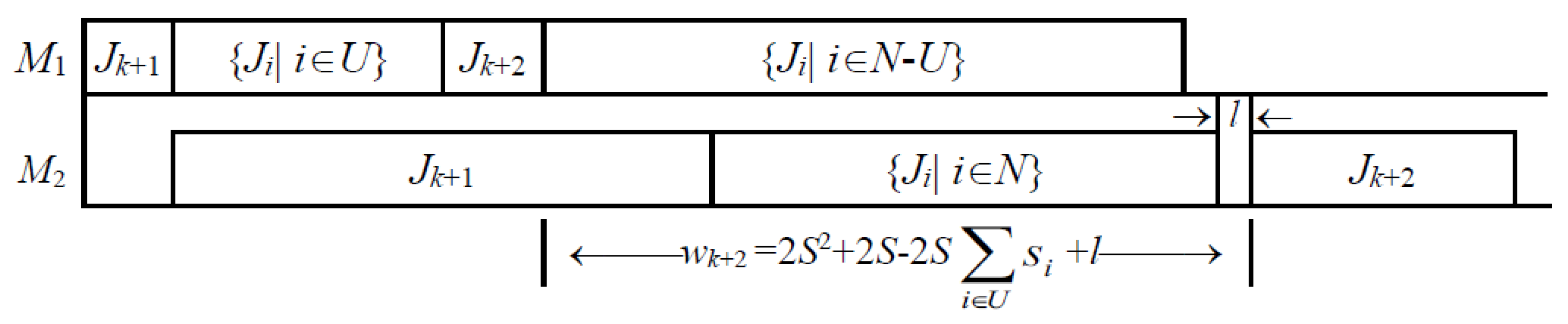
Lemma 3. If Jk+2 is not processed second on machine M1, then the makespan of any schedule is greater than 4S2 + S + 3.
Proof. Let U = {i|Ji is processed between Jk+1 and Jk+2 on machine M1}. If there are jobs Ji, i∈U, then the following two cases are considered:
- (1)
If any job Ji, i∈N, does not create any idle-time slot on machine M2, that is, the processing of these jobs on machine M2 is continuous, then there are two subcases:
- (i)
If 2
S2 + 2
S − 2
S (
Figure 2),
then
where
wk+2 =
bk+1 +
+
l −
−
ak+2 = 2
S2 + 2
S − 2
S +
l and
l ≥ 0.
- (ii)
If 2S2+ 2S − 2S < 0, then Jk+2 creates an idle-time slot lk+2 = 2S − 2S2 − 2S > 0 on machine M2. From Lemma 2, if Jk+1 is scheduled first and there is no idle time on machine M2, except during operation 1 of Jk+1, there is a lower bound of the Cmax, which is 4S2 + S + 3. In this case, Jk+2 creates an idle-time slot lk+2 > 0; therefore, Cmax > 4S2 + S + 3.
- (2)
Similarly, if a job Jr, r∈N, creates an idle-time slot lr > 0, then Cmax > 4S2 + S + 3.
Thus, we only consider the schedules whose Jk+2 is processed second on machine M1. □
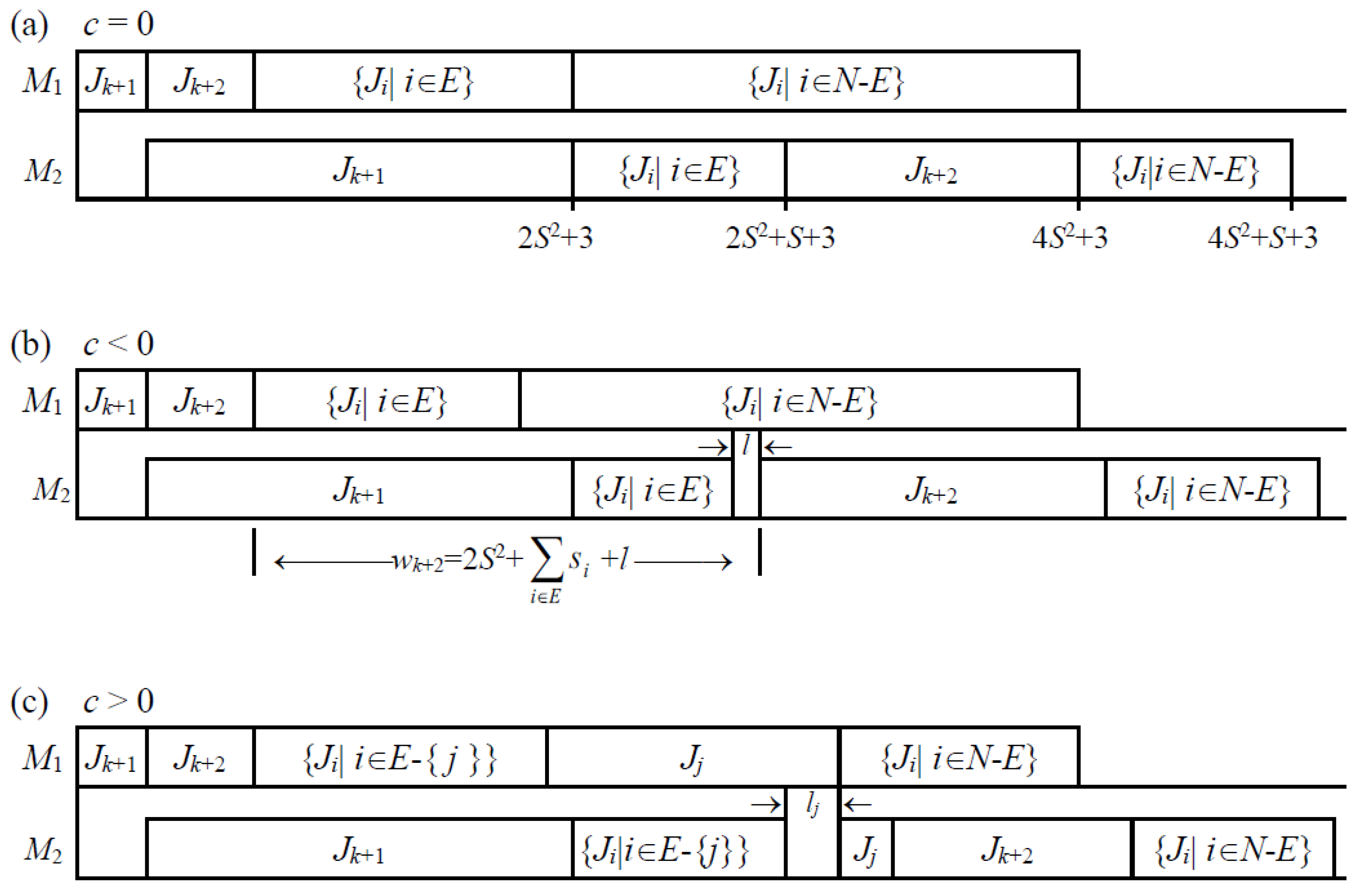
Theorem 1. For any given positive number α > 0, αi = α, i = 1, …, n, the two-machine makespan flowshop scheduling problem T is NP-hard.
Proof. If partition has a solution, then there is an optimal schedule with the makespan
Cmax = 4
S2 +
S + 3 (
Figure 3a). We note that, in this case, the waiting time
wi ≥
di for each
i.
If partition has no solution, we will show that the makespan of any schedule for the above instance is greater than 4S2 + S + 3. For given schedule in which Jk+1 is processed first on two machines and Jk+2 is processed second on machine M1, we let E = {i|Ji is processed between Jk+1 and Jk+2 on machine M2}. By the assumption that partition has no solution and − S = c ≠ 0, we consider the following two cases:
- (1)
If
c < 0 and
l > 0 (
Figure 3b), we have
where
wk+2 =
bk+1 +
+
l −
ak+2 = 2
S2 +
+
l.
- (2)
If
c > 0 (
c ≥ 1/2, because
s1,
s2, …,
sk are positive integers), without loss of generality, we let
Jj,
j ∈
E, be the last processed job in
E (
Figure 3c), then there are two cases:
- (i)
If any job
Ji,
i ∈
E-{
j}, does not create any idle-time slot, then we will show that job
Jj creates an idle-time slot
lj > 0 on machine
M2 (
Figure 3c). The idle-time slot is
Hence, Cmax > 4S2 + S + 3.
- (ii)
If a job Jr, r ∈ E-{j}, creates an idle-time slot lr > 0, then Cmax > 4S2 + S + 3.
Thus, the makespan is greater than 4S2 + S + 3 if partition has no solution. It follows that partition has a solution if and only if the optimal schedule of the above instance has the minimum makespan Cmax = 4S2 + S + 3. □
3. A 0-1 Mixed Integer Programming Formulation
According to the similar analysis in Yang and Chern [
23], a 0-1 mixed integer programming of the problem is developed as follows. First, we denote that
Ai = the starting time of job i on machine M1;
Bi = the starting time of job i on machine M2;
wi = the actual waiting time of job i before its processing on machine M2 = Bi − Ai − ai;
Wi = max{di − wi, 0}= max{di − Bi + Ai + ai, 0};
yijk = 1, if job i precedes job j on machine Mk;
yijk = 0, otherwise;
Cmax = the makespan.
For each job
i, it is clear to have
In addition, it is necessary to assure that no two operations can be processed simultaneously by the same machine. Suppose, for example, that job
j precedes job
i on machine 1, then it is necessary to have
On the other hand, if job
i precedes job
j on machine 1, then it is necessary to have
These inequalities are called disjunctive constraints, because one and only one of these inequalities must hold. In order to accommodate these constraints in the formulation, these disjunctive constraints can be rewritten as follows:
where
M represents a sufficiently large positive number.
By the same way, these disjunctive constraints of job
i and job
j processed on machine 2 can be expressed as follows:
We note that
then it is necessary to have
Wi ≥ 0 and
For the makespan problem, it is necessary to have
Then, a disjunctive integer programming formulation of the proposed problem can be given by
| minimize | Cmax | |
| subject to | Cmax ≥ Bi + bi + αiWi | 1 ≤ i ≤ n, |
| Bi ≥ Ai+ ai | 1 ≤ i ≤ n, |
| Ai + Myij1 ≥ Aj + aj | 1 ≤ i < j ≤ n, |
| Aj + M(1 − yij1) ≥ Ai + ai | 1 ≤ i < j ≤ n, |
| Bi + Myij2 ≥ Bj + bj + αjWj | 1 ≤ i < j ≤ n, |
| Bj + M(1 − yij2) ≥ Bi + bi + αiWi | 1 ≤ i < j ≤ n, |
| Wi ≥ di − Bi + Ai + ai | 1 ≤ i ≤ n, |
| Cmax, Ai, Bi, Wi ≥ 0, 1 ≤ i ≤ n, yijk = 0 or 1, | 1 ≤ i ≤ j ≤ n, 1 ≤ k ≤ 2. |
The total number of type (1), (6), and (7) constraints is equal to 3n. The total number of type (2) and (3) constraints is equal to n(n − 1). The total number of type (4) and (5) constraints is equal to n(n − 1). Hence, the total number of constraints is n(2n + 1). There are 3n + 1 nonnegative variables of Cmax, Ai, Bi, and Wi. We note that if yijk is in the formulation, then yjik needs to be defined. Hence, there are n(n − 1)/2 0 − 1 integer variables of yij1 and the same number of yij2. The total number of variables is thus n(n + 2) + 1.
4. Heuristic Algorithm and Its Worst-Case Performance
As a reducible waiting time is considered in the proposed problem, somehow, the proposed problem is similar to the two-machine flowshop scheduling problem with start and stop lags. Therefore, we first use the Maggu and Das’s algorithm [
27] to determine a sequence
A (Algorithm 1).
| Algorithm 1. Maggu and Das’s algorithm |
Step 1. Let J = {J1, J2, …, Jn}.
Step 2. Determine the job processing order in the following way:
2.1 Decompose set J into the following two sets:
2.2. Arrange the members of set U in nondecreasing order of ai + di, and arrange the members of set V in nonincreasing order of bi + di.
2.3. A sequence A is the ordered set U followed by the ordered set V. |
Some solvable cases are described in the following.
First, if
{α
i}≥1, the proposed problem is the same as that in Dell’Amico [
17]. Therefore, if
{
di} ≤
{
bi +
di} or
{
di} ≤
{
ai +
di}, an optimal schedule is given by Maggu and Das’s Algorithm.
Theorem 2 ([
23])
. In the problem, the case considered here is with {αi}≤1,
{ai + di} ≤ {bi + di}, and ai* +αi*di* = {ai +αidi}. If there is a job Jj, such that aj + dj ≤ bi* +αi*di*, then (Ji*, Jj, B) is an optimal schedule, where B is an arbitrary subsequence of the jobs without Ji*, Jj. Theorem 3 ([
23])
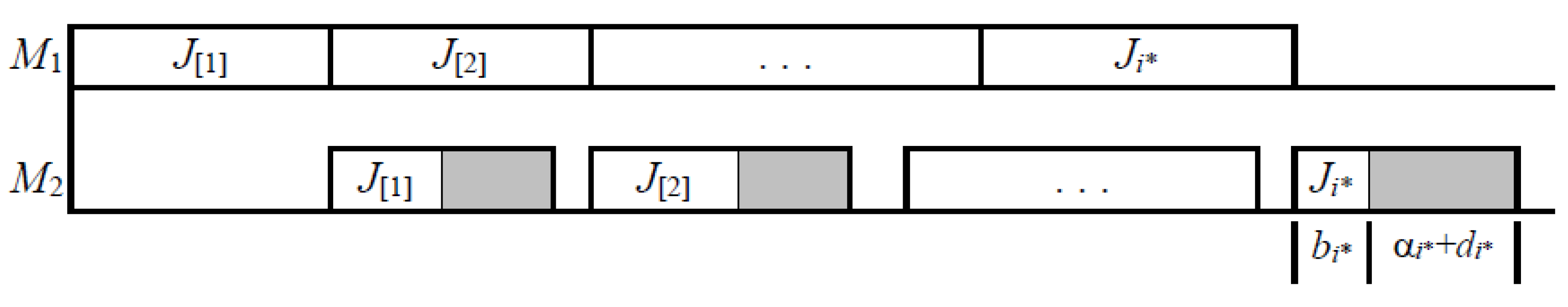
. If {αi} ≤ 1, {ai} ≥ {bi + αidi} and bi* + αi*di* = {bi + αidi}, then (B, Ji*) is an optimal schedule, where B is an arbitrary subsequence of the jobs without Ji*, and we schedule the jobs with no-wait manner as shown in Figure 4. Proof . It is clear that a lower bound on the makespan is
+
{
bi + α
idi}. If
{α
i} ≤ 1,
{
ai} ≥
{
bi + α
idi}, then the makespan of (
B,
Ji*) with no-wait manner, as shown in
Figure 4, is equal to the lower bound
+
bi* + α
i*di*. Hence, (
B,
Ji*) is an optimal schedule. □
In the following, we propose a heuristic algorithm for the problem. The heuristic algorithm is presented for the problem with ai ≥ 0, bi ≥ 0, αi > 0, and di > 0 for all of the jobs. In this problem, if αi ≥ 1, then it is useless to reduce the waiting time. However, if 0 < αi < 1, then it is useful to reduce the waiting time as much as possible. A stepwise description of the algorithm is given as follows (Algorithm 2):
| Algorithm 2. Heuristic algorithm |
- Step 0.
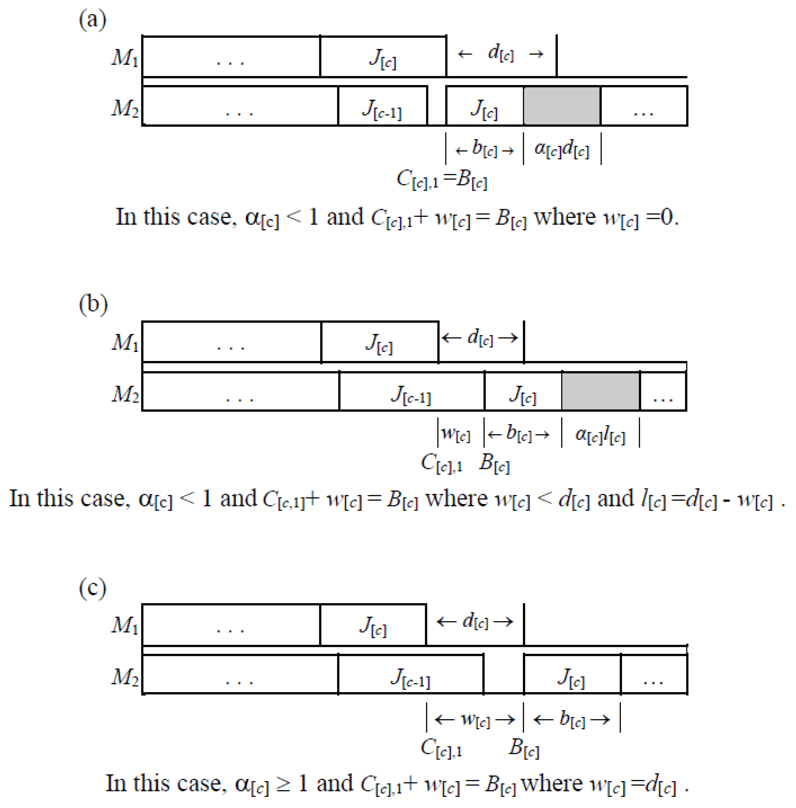
(Initialization) Check those conditions stated in Theorem 2 and Theorem 3. If any one of conditions holds, the optimal schedule is obtained. Otherwise, generate a heuristic solution in the following steps. Determine a sequence π by using Maggu and Das’s algorithm. Set k = 1 and C[0],1 = C[0],2 = 0. - Step 1.
(Determining the reduced period of waiting time and the additional time on machine M2 for each job) Set C[k],1 = C[k−1],1 + a[k]. If C[k−1],2 − C[k−1],1 < a[k] ( Figure 5a), then go to Step 1.1. If a[k] ≤ C[k−1],2 − C[k−1],1 ≤ a[k] + d[k] ( Figure 5b), then go to Step 1.2. If a[k] + d[k] < C[k−1],2 − C[k−1],1 ( Figure 5c), then go to Step 1.3. - 1.1
If 0 < α[k] < 1, then C[k],2= C[k],1 + b[k] + α[k] ⋅ d[k]. If 1 ≤ α[k], then C [k],2 = C[k],1 + d[k] + b[k]. Go to Step 2. - 1.2
If 0 < α[k] < 1, then C [k],2 = C [k−1],2 + b[k] + α[k] ⋅( C[k],1 + d[k] − C [k−1],2). If 1 ≤ α[k], then C [k],2 = C[k],1 + d[k] + b[k]. Go to Step 2. - 1.3
C[k],2 = C [k−1],2 + b[k]. Go to Step 2.
- Step 2.
Set k = k + 1 If k ≤ n, go to Step 1. Otherwise, stop.
|
In the heuristic algorithm, Step 0 first determines a sequence A by using Maggu and Das’s algorithm. Step 1 adjusts the reduced period of waiting time and the additional time on machine 2 for each job. In Step 1.1 and Step 1.2, if α[k] ≥ 1, then it is useless to reduce the waiting time. However, if 1 > α[k] > 0, then it is useful to reduce the waiting time as much as possible and the calculation of the completion times on both machines is given. Step 1.3 depicts that if a[k],1 + d[k] < C [k−1],2 − C [k−1],1, then it is useless to reduce the waiting time either α[k] ≥ 1 or 1 > α[k] > 0.
In the following, an example of five jobs is given to illustrate the heuristic algorithm.
Example 1. There are five jobs; that is, J1, J2, J3, J4, and J5, to be processed on machine M1 and machine M2. The processing times of these jobs on machine M1 are a1 = 1, a2 = 3, a3 = 2, a4 = 3, and a5 = 2, respectively. The processing times on machine M2 are b1 = 5, b2 = 4, b3 = 1, b4 = 2, and b5 = 3, respectively. The delay times required before its processing on machine M2 are d1 = 2, d2 = 3, d3 = 1, d4 = 2, and d5 = 5, respectively. The cost indices are α1 = 0.2, α2 = 0.3, α3 = 0.1, α4 = 0.5, and α5 = 1.2, respectively.
According to the above heuristic algorithm, we obtain that the makespan of these five jobs is 16.6. Please see the details in
Appendix B.
Lower bound
First, we assume that processing on each machine may be continuous,
D1 = {
i?α
i ≥ 1 for
iN} and
D2 =
N–
D1. We can see that, if α
i ≥ 1, then it is useless to reduce the waiting time. However, if 1 > α
i > 0, then it is useful to reduce the waiting time as much as possible. Because all the jobs have to be processed on machine
M1 and
M2, if the delay time is short relative to the corresponding processing time, we have an immediate lower bound
LB1 =
max {
+
min {
{
di +
bi},
{α
idi +
bi}},
min {
{
ai +
di},
{
ai + α
idi}}+
}. On the other hand, if one of the delay times is long enough relative to the corresponding processing time, we have the second lower bound
LB2 =
max {
{
ai +
di +
bi},
{
ai + α
idi +
bi}}. Hence, a lower bound is calculated as follows:
In the following, we will find the worst case of the heuristic algorithm. First, some notations are defined. Given a solution of the proposed problem, we define the critical job as the job with maximum starting time on machine M2, such that , where and , , , and are the completion time of on machine M1, the delay time of , the actual waiting time of , and the starting time of on machine M2, respectively. We also define JP as the set of jobs proceeding on machine M1, and JF as the set of jobs following on machine M2. Then, considering the schedule in which the jobs are arranged by Maggu and Das’s algorithm, there are three cases of the makespan, as follows.
- Case 1.
and
(See
Figure 6a)
- Case 2.
and
(See
Figure 6b)
- Case 3.
Theorem 4. Let π* be an optimal schedule and π be the Maggu and Das’s schedule for the heuristic algorithm. Ifand, thenand the bound is tight.
Proof. Considering the schedule in which the jobs are arranged by Maggu and Das’s algorithm, if
and
, then the makespan is as follows:
Therefore, if
, the jobs
JP have the property of
. Then, we have the following results:
Similarly, if
, the jobs
JF have the property of
. Thus,
Hence, .
To prove the tightness of the bound, consider with , , , and , and () with , , , and . By applying Maggu and Das’s algorithm, the job sequence is on both machine M1 and M2. Then, .
On the other hand, an optimal schedule can be obtained by arranging the job sequence on machine M1 and the job sequence on machine M2. Then, . Hence, , which tends to 2 as n → ∞. □
Theorem 5. Let π* be an optimal schedule and π be the Maggu and Das’s schedule for the heuristic algorithm. If, thenand the bound is tight.
Proof. The proof is the similar to that of Theorem 4. Thus, we omit it here. □
5. Computational Experiments
Although we find the worst case of the heuristic algorithm under some certain situations (case 1 and case 3), the upper bound of case 2 is still unknown. Therefore, in order to evaluate the overall efficiency of the heuristic algorithm, we generate several groups of random problems as follows:
- (1)
n is equal to 10, 20, 30, 40, 50, 60, 70, 80, 90, 100, 150, 200.
- (2)
ai is uniformly distributed over [1,100].
- (3)
bi is uniformly distributed over [1,100].
- (4)
αi is uniformly distributed over [1,2].
- (5)
di is uniformly distributed over [0,50], [50,100], or [100,200] depending on the group.
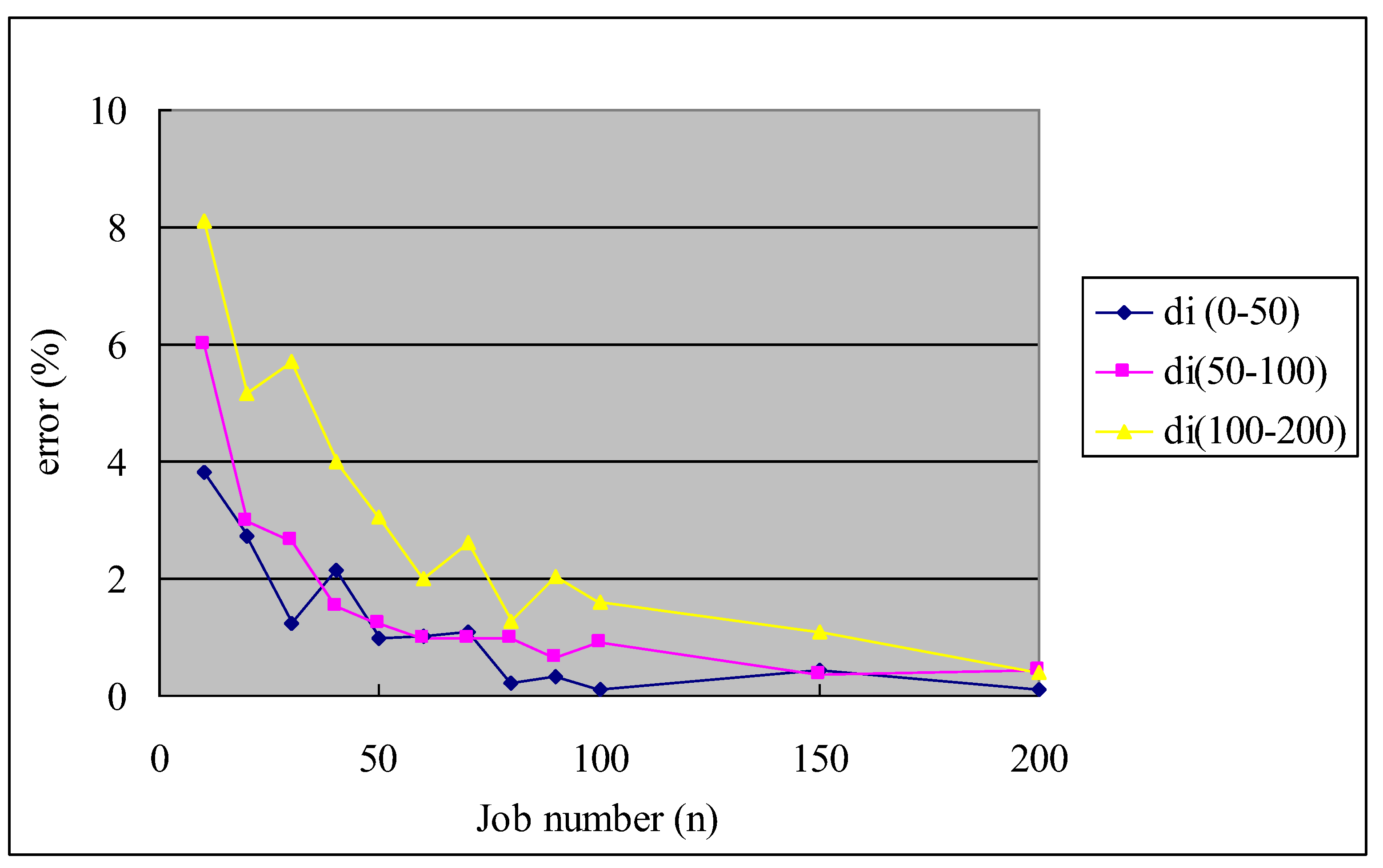
In the computational experiment, a total of 720 test problems are generated. The computation times of algorithms for all the test problems are within one second. For each of these random problems, the percentage of the error e = (Ch − Clow) ∗ 100/Clow is computed, where Ch is the makespan of the heuristic solution and Clow is the lower bound on the makespan.
The result is given in
Table 1. There are 20 test problems for each problem type. To evaluate the overall performance of the heuristic algorithm, we compute the mean of all the average percentage errors reported in
Table 1. The mean value is 1.97%, which suggests that the heuristic algorithm, on average, finds schedules that are within 1.97% of optimality. From Theorem 4 and 5, we can see that the upper bound of the heuristic algorithm is
; therefore, the performance of the heuristic algorithm is quite satisfactory. From
Figure 7, the larger the value of
di, the greater the percentage of the error. Because the proposed heuristic algorithm is restricted to searching a near-optimal permutation schedule, it may imply that the optimal schedule is likely to be a non-permutation schedule when the values of delay times of jobs are larger. Therefore, the performance of the heuristic algorithm is better when
di is smaller. We can also see that the average percentage of errors decreases as the job number
n increases for different values of
di. Especially, when the job number
n is more than 100, the mean value of the average percentage of errors is less than 1%. In view of the NP-hardness of the problem, this result is quite encouraging as it provides efficient procedures for solving large-sized problems.


