Analysis of Environmental Productivity on Fossil Fuel Power Plants in the U.S.

Abstract

In 2007, the Clean Air Act officially included greenhouse gases, making fossil fuel power plants the first of key industries regulated by the Environmental Protection Agency. How do we measure the impact of the regulations on these power plants’ productivity? Previous studies that attempt to answer this question have provided inadequate answers because their samples cover the periods only up to 2007, and they often use greenhouse gases as the only proxy for the undesirable output. This paper collects data from 133 fossil fuel power plants in the United States and covers 2004 to 2013. These power plants are divided into Sun Belt and Frost Belt based on their geographical locations. To measure the undesirable outputs, we used both carbon dioxide and toxic emissions as the proxies. The estimation model includes the construction of a generalized common stochastic frontier (metafrontier) and a Malmquist productivity index. We used the index to measure the change in productivity for the power plants before and after the implementation of the regulation. The results indicate that, since regulation in 2007, the overall production efficiency of the power plants has declined incessantly while productivity has seen a sustained downward trend despite two surges in growth.

1. Introduction

Industrial development affords people convenience, comfort, and abundance; however, it has also caused irreversible environmental damage. Environmental degradation has affected not only the survivability of other species, but it has also threatened human health and survival. In recent years, one can easily witness environmental counterattacks. The effects have become self-evident: The greenhouse effect, ubiquitous heavy metal waste, acid rain, and air pollution. According to the World’s Worst Pollution Problems Report, approximately 120 million people worldwide are constantly exposed to environmental toxic risks, and approximately 17 million people are directly affected by industrial pollution each year [1]. In order to control and manage pollution, countries around the world have signed various environmental agreements since 1992. Such agreements include the United Nations Framework Convention on Climate Change and the Basel Convention on the Control of Transboundary Movements of Hazardous Wastes and Their Disposal, usually referred to as the Basel Convention.

Although protecting the environment has become a worldwide consensus, industrialized countries bear a greater responsibility for damaging the environment, and they ought to assume a commensurate role in protecting it. The advanced economies of today generally developed earlier, in an era when the environmental repercussions of human activity were slim—and regulations were equally as slim. Likewise, emerging economies developed relatively later, fueled by commodity processing and heavy industry. Unsurprisingly, these peoples are subject to graver pollution effects [2]. As the understanding of environmental degradation increased, so, too, did regulations. This means that to pursue industrialization, emerging countries need to bear higher environmental costs and corresponding investment to achieve an equal level of development, comparative to the beginnings of industrialization for currently developed countries. China is a typical case. Gao, Yang, Yang and Yuan [3] showed that China’s rapid output growth is dependent on substantial energy consumption, which is accompanied by large pollution emissions. This also promotes significant investment in pollution mitigation. Between 2000 and 2017 in China, the annual total energy consumption increased more than two times, from approximately 1.5 to 4.3 billion tons of standard coal. Meanwhile, the total investment in pollution control increased by more than 5.5 times, from approximately 170 to 950 billion RMB. Among the industrialized countries, the United States has long benefited from industrial development and has played a leading role in the global economy and political theatre. Being the second largest producer of greenhouse gases in the world, the U.S.’ willingness and attitude toward environmental protection has a far-reaching effect. Indeed, the U.S. has invested considerable efforts and resources in improving the environment (according to Statistics International Energy Agency [4], the top five greenhouse gas emission countries are China, the United States, India, Russia, and Japan. In total, 16% of carbon emissions from energy consumption in the world comes from the U.S. [5]). The Supreme Court ruling that greenhouse gases are pollutants under the Clean Air Act has provided the legal support for government interventions. As such, this has required companies to provide data on the emission of greenhouse gases (even though the treaty has not been signed, the U.S.’ attitude toward reducing greenhouse gas control is apparent). It has also produced the Toxics Release Inventory, a list with various types of toxic waste (this was based on the Clean Air Act, the Clean Water Act, and the Resource Conservation and Recovery Act), which mandates that manufacturing and high-polluting enterprises must report their emissions and their disposal processes.

Fossil fuel power plants are categorized as a high-polluting industry. In the U.S., greenhouse gas and toxic waste account for 32% and 13% of total emissions, respectively [5]. They become the focus of relevant regulations. For example, to regulate air pollution in 1970 and 1990, the Clean Air Act designated the fossil fuel power plant industry as the first to bear the brunt. Sueyoshi and Goto [6] pointed out in their empirical study, with data spanning from 1995 to 2007, that the Clean Air Act had significantly curtailed greenhouse gas emissions from the fossil fuel power plants. Furthermore, they noticed that Clean Air Act regulation on emissions has an increasing impact over time. The Environmental Protection Agency has clearly played a crucial role in protecting the environment. In 2011, it directly restricted the emission of harmful substances, such as mercury, from fossil fuel power plants, in accordance with the Clean Power Plant Act. In 2013, the Environmental Protection Agency proposed the facility requirements and carbon emission standards for new fossil fuel power plants. In 2014, and based on the Climate Action Plan, the Environmental Protection Agency put forward a clean energy plan requiring a reduction in carbon pollution from existing fossil fuel power plants. Through intensive policies and regulations, greenhouse gas and toxic emissions of the fossil fuel industry have decreased over the years [5].

Pollution prevention and economic development are similar in behavior to a seesaw. When environmental awareness becomes the darling of policy and public opinion, the additional cost to reduce pollution seems to come at the displeasure of the industry. The literature on the efficiency and productivity of the American fossil fuel power plants, however, seems to focus research on the period before 2007 [6,7]. There are four reasons why research on the period after 2007 is worthwhile and perhaps even more important. The first reason is related to the attitude toward environment protection. A majority of countries in the world signed into the Kyoto Protocol on February 16 2005 (the Kyoto Protocol is an amendment to the United Nations Framework Convention on Climate Change), with a goal of jointly controlling greenhouse gases. The U.S. withdrew from this protocol shortly after because of concerns over its economy and other related factors. The decision by the U.S. immediately drew international attention and criticism. In practice, however, the U.S. government has substantially strengthened the control of greenhouse gases since 2007, which has resulted in long-lasting impact on fossil fuel power plants. Naturally, it is essential to explore and discover policy impacts and industry responses beyond 2007. In recent years, other countries have been paying more attention, from a policy and academic perspective, to environmental issues. Specific to policies, countries around the world have gradually strengthened the relevant regulations. Yang, Yuan, and Han [8] showed that aside from the United States, countries, such as the United Kingdom, Australia, Mainland China, Hong Kong, and India, have implemented strict air quality assessment systems. Academically, a large number of studies center on the efficacy of environmental regulations, with most of the focus being on China. For example, Yang and Li [9], Yang, Yuan and Han [8] and Yuan and Yang [10] took aim at China’s air pollution. Hu, Jin, and Kavan [11] put the focus on China’s heavy metal pollution. Pettersson and Soderhölm [12] reviewed the licensing processes of Swedish regulatory design to assess the effectiveness of industrial pollution control. As for the empirical studies that directly concern the environmental productivity of fossil fuel power plants after 2007, the number is not many and most of them focus on China. For example, Zhang, Kong, Choi, and Zhou [13] adopted non-radial directional distance functions with data in 2011 to examine the effect of a size control policy on energy and carbon efficiency for the Chinese fossil fuel power industry. Zhang and Choi [14] used the metafrontier non-radial Malmquist performance index with data from 2005 to 2010 to measure the dynamic changes in total factor CO₂ emission for Chinese fossil fuel power plants. Zhang, Zhou and Choi [15], with a 2011 dataset, conducted the metafrontier non-radial directional distance function to compare the total factor energy efficiency and CO₂ emission performance for Korean coal-fired and oil-fired power plants. However, research that is directly aimed at the environmental productivity of fossil fuel power plants in the United States after 2007 iseven rarer. Sueyoshi and Goto [16] produced the only article using data envelopment analysis (DEA) radial measurement to evaluate the environmental efficiency for fossil fuel power plants in the U.S. with a 2009 dataset.

Secondly, this paper proposes a new approach to measuring the variables. To put the industrial impacts on the environment within the context of efficiency or productivity analysis, the typical approach is to treat the by-product that has adverse effects on the environment as undesirable outputs [13,17,18]. The by-product is often measured by air pollutants, such as carbon dioxide or sulfur dioxide [6,7,19]. The undesirable by-products in the case of fossil fuel power plants, however, not only include air pollution but also the production of non-gaseous hazardous substances, such as hydrochloric acid, barium compounds, and mercury. The resulting damage from these chemical by-products has drawn a lot of attention in recent years and should be included in the analysis.

The third reason driving this paper concerns the research methods used in prior studies. An important reason to study environmental efficiency and productivity is to find a solution for reducing the undesirable output without affecting economic development. Unfortunately, there is no satisfactory answer to this question when using the model given by the traditional production function. In recent years, the academic community has made considerable progress in this regard. Färe and Grosskopf [20] developed a directional output distance function by applying the concept of expansion and contraction of Shephard’s [21] distance function to maximize the desirable output, holding factor inputs and undesirable output constant. Cuesta and Zofio [22] extended the model to a circumstance where the expansion of desirable output and reduction of undesirable output coexist and thereby developed an estimation method with the hyperbolic distance function (this estimation method can reflect the production technology for environmental improvement. It can also avoid the problem caused by the selection of directional vectors [23]).

The fourth reason for this paper concerns the model specification. Previous research usually estimates efficiency and productivity first. The results are then classified into groups for comparison purposes using different attributes or characteristics. For example, the power plants can be classified into the Sun Belt group and the Frost Belt group (relevant research includes [24,25,26,27]), according to location. This implies that power plants with different characteristics can fall into the same group with a presumed identical technological frontier. To solve the misspecification problem caused by superimposing all plants on an identical production frontier, Battese et al. [28] expounded the concept of the common frontier (metafrontier) and solved the model with a nonparametric linear programming method. Subsequently, Huang, Huang and Liu [29] extended the model to a parametric stochastic common boundary architecture, which has significantly improved the operability of statistical methods.

The novelty and contribution of this paper are based on the four factors mentioned above: Environmental legislation, variable measurement, estimation method, and model specification. Among these, both greenhouse gases and toxic substances, which are listed in the Toxics Release Inventory, are the pollution variables. The hyperbolic distance function proposed by Cuesta and Zofio [22] is the main estimation method, with a reference to [24,25,26,27]. To apply the stochastic metafrontier of Battese et al. [28] and Huang, Huang and Liu [29], locations of fossil fuel power plants are divided into the Sun Belt and Frost Belt. Throughout the paper, empirical analysis is supplemented with observations on how productivity has evolved from 2004 to 2013 for fossil fuel power plants as a result of the U.S. environmental policies and regulations that were enacted.

The rest of the paper is organized as follows: Section 2 is the literature review. It covers issues related to U.S. environmental regulations, the method of environmental performance evaluation with undesirable output, and the application of the distance functions to research related to the environmental productivity of fossil fuel power plants. Section 3 introduces the methodology, including how to take into account the undesirable outputs, formulation of the distance functions, specification of the metafrontier framework for assessing productivity, and construction of variables for empirical analysis. Section 4 presents the empirical findings with a comparative analysis of the environmental efficiency and productivity of U.S. fossil fuel power plants. The last section provides a summary and conclusion to this paper.

2. Literature Review

2.1. U.S. Environmental Regulations and Related Research

In the U.S., there are six types of regulations related to environmental issues. These include the Clean Air Act, the Clean Water Act, the Resource Environmental Protection and Recycling Act, the Safe Drinking Water Act, the Comprehensive Environmental Response, Compensation, and Liability Act, and the Superfund Amendments and Reauthorization Act. Among them, the Clean Air Act made the most significant impact because pollution caused by fossil fuel power plants is mainly through air.

U.S. legislation on air originated from the Air Pollution Control Act of 1955, a law intended to provide federal funding for research on air pollution. The Clean Air Act of 1963 began to regulate air pollution. To establish a national standard on air quality, the Clean Air Act was revised in 1970 to incorporate the New Source Performance Standards for specific industries, which imposes restrictions on production technology with new facilities, and substantially expands the power of the Clean Air Act in regulating pollution emissions. The New Source Review was further developed in 1977, requiring new facilities to pass the environmental specification review of the Environmental Protection Agency before construction.

In 1990, the Clean Air Act also began to participate in the discharge control of 189 toxic substances that would cause air pollution, such as acid rain and haze. The regulation requires that pollution-producing enterprises must obtain the right to operate after being issued a permit. In 2007, the U.S. Supreme Court ruled that the Clean Air Act should cover the relevant regulations for greenhouse gases and give the Environmental Protection Agency the power to control emissions. In 2010, the Environmental Protection Agency mandated polluting enterprises to report data on greenhouse gas emissions, based on the greenhouse gas reporting plan promoted by the 2008 Comprehensive Appropriations Act. In 2011, based on New Source Performance Standards, the Environmental Protection Agency introduced Mercury and Air Toxics Standards to limit emissions of heavy metals, such as mercury and arsenic, from existing power plants (the largest source of mercury emission is fossil fuel power plants, accounting for 50% of pollutants in the U.S. [30]).

The bills and regulations mentioned above do have a substantial impact on the power plant industry. Rubin, Taylor, Yeh, and Hounshell [31] pointed out in the study of the environmental technology learning curve that, after 1970, many coal-fired power plants chose to install a flue gas desulfurization system to reduce sulfur emissions to meet the revised standards of the Clean Air Act. Furthermore, all new coal-fired power plants established after 1978 used the same system to control sulfide emissions. Adair, Hoppock, and Monast [32] indicated that, after the greenhouse gas control was included into the Clean Air Act, 75% of coal-fired power plants failed to meet the New Source Review standards instigated by the Environmental Protection Agency, which based the regulations on the total amount of emissions instead of the ratio. The introduction of regulations on greenhouse gas has resulted in a significant upgrade of the equipment for coal-fired power plants. Interestingly, however, even though pollution has been effectively suppressed, overall economic benefits have not necessarily improved. Fleishman et al. [33] showed that between 1994 and 2004, strict environmental regulations reduced coal combustion. The loss of efficiency and productivity of power plants clearly offsets the benefits of reducing emissions.

2.2. Environmental Performance Assessment

The literature uses different words to define environmental performance, but the content described is roughly the same. Klassen and McLaughlin [34] defined environmental management as taking into account the negative impact on the environment during the production process. Therefore, environmental performance can be defined as the degree of pollution that the enterprise controls in the production process. Keffer, Shimp and Lehni [35] argued that environmental performance refers to the interrelationship between economic and environmental (ecological) values. Verfaillie and Bidwell [36] defined environmental performance as reducing the damage to the ecological environment, caused by the production of products and the loss of resources, while also reducing the impact to Earth to an acceptable level. Under these narratives, the definition of environmental performance can be summarized as the search for a balance between economic output and the environment—that is, to pursue output growth without affecting the environment.

Under this definition, and in order to effectively evaluate environmental performance, previous research often relied on “undesirable output” and “distance function”. In terms of “undesirable output”, Färe, Grosskopf, Lovell and Pasurka [37] explained that production activities in general can produce “desirable output” as well as “undesirable output”. Undesirable output may include environmentally harmful substances, such as wastewater and waste material, and it takes additional costs to clean up or control. Manufacturers may lack the incentive to take action if the cost they incurred only improves pollution but fails to produce economic benefit. Therefore, the research model for assessing environmental efficiency often sets the goal of increasing the desirable output while minimizing undesirable output [38,39,40].

However, there is a trade-off in the undesirable output. Färe and Grosskopf [20] pointed out in their study on the shadow price of sulfur dioxide emissions from power plants that undesirable output can be reduced either by investing in additional equipment to improve the production technology, or by directly reducing the scale of output—this is, the “weak disposability” of undesirable output. The power plant can also choose the production quantity and efficiency that it intends to produce—that is, a choice on the spectrum between pollution and purity. This is the “strong disposability” of the desirable output.

The measurement of undesirable output is quite straightforward. Murty et al. [38] applied emissions data of sulfur dioxide, aerosols, and nitrogen oxides to measure the impact of Indian coal-fired power plants on air pollution. Sueyoshi and Goto [6] measured the environmental efficiency of U.S. power plants using emissions data for sulfur dioxide, CO₂, and nitrogen oxides. Kumar and Managi [7] used emissions data for sulfur dioxide and nitrogen oxides to measure changes in productivity in U.S. fossil fuel power plants. Wei, Loschel and Liu [41] applied carbon dioxide data to directly measure the impact of changes in the size and age of Chinese power plants on environmental efficiency. In general, the literature relies on the quantity of air pollutants as a measure of the undesirable output produced by fossil fuel power plants. In addition to air pollutants, fossil fuel power plants have produced other byproducts, such as mercury-containing wastewater and other waste material, which are often overlooked in environmental efficiency studies.

There are two ways to measure efficiency related to the undesirable output. One is to evaluate the production efficiency of the desirable output by treating the undesirable output as an input of the production function [42]. Ramanathan [43] used data envelopment analysis and consider carbon dioxide as a reducible input when estimating the extent to which carbon dioxide affects gross domestic product in various regions of China. The advantage of this approach is that it is easy to estimate while the disadvantage lies in the inconsistency of the logic. The input of carbon dioxide does not bring about gross domestic product, and the production process does not actually use carbon dioxide. The other way to measure efficiency is to treat the undesirable output as a reducible and controllable output [44,45,46]. This approach specifies its model to be logically consistent with the production practice, but the estimation is relatively complicated.

The evaluation model of environmental efficiency is often carried out by using stochastic frontier analysis and data envelopment analysis. Data envelopment analysis uses linear programming to directly calculate the envelop production frontier of all decision-making units, and estimates the efficiency value of relative frontiers. The advantage of data envelopment analysis is that the estimation is based on mathematical programming; it requires only a small sample and is suitable for the case of multi-input and multi-output. The disadvantage of data envelopment analysis lies in choosing the weights for input and output. Stochastic frontier analysis is based on regression, assuming that the output falls on the production frontier with a margin of error, to estimate the efficiency value of the relative frontier. The advantage of stochastic frontier analysis is that it allows for stochastic error and the relationship between the input and output can be clearly defined. The disadvantage is that the statistical model requires a large sample and is limited to one input and one output. To ease this restriction, previous research has introduced the distance function method.

The principle of the distance function method is to scale the input and output of the decision-making unit to its production frontier. Therefore, it is suitable for measuring multiple inputs and multiple outputs. Given the inputs, one is to maximize the output-oriented distance function. Alternatively, given the outputs, one is to minimize the input-oriented distance function [21]. There are two ways to extend this concept to the undesirable output: The directional or hyperbolic distance function method.

Regarding the former, Chung et al. [17] converted the distance function to direction vectors so that the undesirable output can be rescaled into the production function to measure environmental efficiency. Färe et al. [44] suggested that the distance function should be given a specific direction vector, and by means of simulating the scenario of maximizing the desirable output while simultaneously reducing the undesirable output. Hence, they developed the directional distance function. Since then, the directional distance function has often been applied to research on environmental performance [7,47,48,49]. In practice, however, using the directional distance function has a potential limitation: It requires an a priori assumption about the undesirable output for adjusting the direction vectors of the desirable and undesirable output. In the case of multiple undesirable outputs, different selections of a priori measurement often produce inconsistent results. To date, the literature still lacks a consensus on the criteria for selection.

Regarding the second extension of using the distance function, Cuesta et al. [23] proposed a hyperbolic curve where expansion or reduction can multiply to describe the scenario of simultaneous expansion in desirable output and contraction in undesirable output. This approach can reflect an improvement of environmental technology and depict the environmental impact of a change in production technology. Yang et al. [46] extended the hyperbolic distance function to allow for maximizing capital input and minimizing energy input and the undesirable output. They used the model to examine how Chinese environmental efficiency could have changed due to government subsidies targeting energy conservation and emission reduction. Relative to the directional distance function method, the hyperbolic distance function method eliminates the need and problem associated with the selection of undesirable outputs.

2.3. Research on the Environmental Performance of Fossil Fuel Power Plants

In the literature, research on the environmental performance of fossil fuel power plants often takes regional differences into consideration. This is especially true for U.S. power plants. The U.S. is a vast territory and the law enforcement agencies in each region are independent from each other. As a result, there are differences in the recognition of law by enforcement personnel, availability of state resources, as well as subjectivity in the strictness and discretion of the regulations and policies. These factors explain variations between the regions in monitoring the environment. For the same reason, the Environmental Protection Agency divides the country into 10 regions and maintains an office in each district [50]. Zwickl, Ash and Boyce [51] pointed out further in their study that each region has different income levels, ethnicities, and education levels that comprise their population. The severity of pollution in each region is a reflection of these differences. They reported that the three most polluted regions in the U.S. are the Midwest, Midsouth, and Mid-Atlantic.

Färe et al. [26] observed that the environmental efficiency of the Frost Belt has slightly improved compared to the Sun Belt. Lee [47] calculated the marginal cost of reducing sulfur for the Great Lakes, Midwest, South, and Northeast districts, and found the Great Lakes region to have the highest marginal cost. Fleishman et al. [33] studied how air quality policy may affect the environmental efficiency score of power plants scattered all over eight U.S. census regions, and they found that regional differences matter. Färe et al. [27] grouped the U.S. into the Sun Belt and Frost Belt and discovered that the Frost Belt has greater environmental performance. Earlier, Färe et al. [25] also pointed out that manufacturing productivity growth in the Frost Belt is greater than in the Sun Belt.

If regional differences reflect environmental production conditions, then manufacturers in different regions will face varied production and technical conditions [52]. Their observation can be applied to the power plant industry as well. Battese and Rao [53] argued that using the same frontier to estimate the efficiency of plants belonging to different technology groups would encounter the risk of specification bias. To mitigate this risk, they proposed a metafrontier framework and recommended a two-stage estimation method. The first stage is to estimate the group frontier with stochastic frontier analysis. The second stage is to estimate the metafrontier with linear programming using the estimates from the previous stage. Later, Huang et al. [29] proposed a stochastic metafrontier method and incorporated the calculation of the metafrontier in the second stage into the stochastic frontier analysis. This method has significantly improved estimation of the metafrontier, as it recognizes the stochastic error that is ignored by linear programming. Another benefit of this method is that it avoids the potential problem of obtaining an efficiency estimate that is greater than one.

In recent years, the metafrontier framework has been widely used in environmental performance assessment. Oh [54] divided 46 countries into three groups, America, Europe, and Asia, and measured the difference in environmental performance with the metafrontier approach. The results show that European countries are the most innovative, ahead of others in environmental productivity, while Asian countries are quickly catching up. Chiu, Liou, Wu and Fang [55] used national competitiveness and sources of income to group countries and studied their environmental efficiency. Zhang and Choi [18] examined the environmental productivity of fossil fuel power plants located in Korea and China. They applied the metafrontier method and measured the gap between the two countries. They found a significant difference in CO₂ emissions between the two countries. They also concluded that China shows a stronger ability in technological leadership while Korea displays greater improvement through technological innovation. In a related paper, Zhang and Choi [14] separated Chinese fossil fuel power plants into two groups: Central and local jurisdiction plants. The empirical results indicated that the centrally managed power plants have a heightened ability to catch up with technology while locally managed power plants have higher efficiency when it comes to innovation.

Interestingly enough, research on environmental efficiency has also been extended to developing the environmental productivity index for fossil fuel power plants; in which, technical efficiency is a static performance assessment, measuring only short-term phenomenon, while the productivity index involves a synthesis of efficiency improvement, technological change, and adjustment of the scale efficiency. It tracks intertemporal and longer-term changes. Therefore, the productivity index is often used in the study of long-term influencing factors, such as changes in regulatory policies. Yaisawarng and Klein [56] were first to incorporate the concept of undesirable output into the Malmquist productivity index to measure productivity changes of the U.S. fossil fuel power plants between 1985 and 1989. They showed that since 1985, productivity declined in three consecutive years before showing a slow tendency towards improvement. To measure productivity changes for the Swedish paper industry, Chung et al. [17] used the method of directional distance function. They measured undesirable output with biological oxygen demand and chemical oxygen demand. Additionally, they expanded the Malmquist productivity index to the Malmguist–Luenberger index. Recently, Zhang and Choi [18] also used the Malmquist productivity index to measure changes of carbon dioxide productivity in China. They found that carbon dioxide emission has an upward trend, which is perhaps a result of ineffective government policies in promoting carbon reduction.

3. Methodology

3.1. Metafrontier and Distance Function

To construct the production frontier for measuring environmental performance, this paper adopts the two-stage stochastic metafrontier method proposed by Huang et al. [29] and Huang et al. [57]. Since the aim of the estimation framework is to maximize the desirable output while minimizing the undesirable output, we must take into account the undesirable output and use the hyperbolic distance function proposed by Cuesta et al. (2009). We first assume that there are k power plant groups, the production technology level, T_t^k, is represented by the group frontier, and the i-th power plant input, x_it, in group k can produce the desirable output, y_it^d, and the undesirable output, y_ijt^u:

$$\begin{array}{l}{T}_t^k=\left\{\left(x_{imt},y_{it}^d,y_{ijt}^u\right):x_{it}canproduce\left(y_{it}^d,y_{ijt}^u\right)\right\},\\ andi=1,2,\dots N^k;j=1,2,\dots ,J^k;m=1,2,\dots ,M^k\end{array},$$

(1)

where the superscript d represents desirable, u represents undesirable, the subscript j of y_ijt^u represents the j-th undesirable output, and the subscript m represents the m-th input. The setting above can be extended to a metafrontier and is written as:

$$\begin{array}{l}{T}_t^{*}=\left\{\left(x_{imt},y_{it}^d,y_{ijt}^u\right):x_{it}potentiallycanproduce\left(y_{it}^d,y_{ijt}^u\right)\right\}\\ ,andi=1,2,\dots n;j=1,2,\dots n\end{array}.$$

(2)

Based on the definition of environmental efficiency mentioned above and the concepts proposed by Färe et al. [36] and Cuesta et al. [23], the distance function of group k conditioning on maximizing the desirable output and minimizing the undesirable output can be written as:

$$D_{it}^k\left(x_{imt},y_{it}^d,y_{ijt}^u\right)=\inf \left\{1>\theta >0:\left(x_{imt},y_{it}^d/\theta ,y_{ijt}^u\theta \right)\in P\left(x_{imt}\right)\right\}.$$

(3)

Equation (3) is also called the group technical efficiency measured by the group frontier. Likewise, the distance function of the metafrontier can be defined as:

$$D_{it}^{*}\left(x_{imt},y_{it}^d,y_{ijt}^u\right)=\inf \left\{1>\theta >0:\left(x_{imt},y_{it}^d/\theta ,y_{ijt}^u\theta \right)\in P\left(x_{imt}\right)\right\}.$$

(4)

Equation (4) is also called the metafrontier technical efficiency measured by the metafrontier. According to Huang et al. [29], the relationship between the group frontiers and metafrontier can be expressed as:

$$\ln D_{it}^{*}\left(x_{imt},y_{it}^d,y_{ijt}^u\right)=\ln D_{it}^k\left(x_{imt},y_{it}^d,y_{ijt}^u\right)+\ln TG{R}_{it}.$$

(5)

Equation (5) indicates that under the common distance function, D_t*(x_imt, y_it^d, y_ijt^u), there is a group distance function, D_t^k(x_imt, y_it^d, y_ijt^u), and a technology gap ratio (TGR); that is, the distance between the group frontier and the common frontier. The result from the first-stage stochastic frontier estimation of the group distance function is D_t^{^k}(x_imt, y_it^d, y_ijt^u), and its relationship with the group distance function, D_t^k(x_imt, y_it^d, y_ijt^u), is:

$$\ln D_{it}^k\left(x_{imt},y_{it}^d,y_{ijt}^u\right)=\ln D_{it}^{^k}\left(x_{imt},y_{it}^d,y_{ijt}^u\right)+{\nu }_{it}^{*},$$

(6)

where ν* is the estimation residual, and ν* = ε^k-ε^{^k}. Huang et al. [57] pointed out that this estimation error does not have to be zero if the number of observations is not infinite. Therefore, the estimated error, ν*, can also represent a random error under a metafrontier. Equation (5) can be rewritten as:

$$\ln D_{it}^{^k}\left(x_{imt},y_{it}^d,y_{ijt}^u\right)=\ln D_{it}^{*}\left(x_{imt},y_{it}^d,y_{ijt}^u\right)+{\nu }_{it}^{*}-\ln TG{R}_{it}.$$

(7)

According to Battese and Coelli [58], in the first stage of estimating the group frontier, factors contributing to inefficiency are firm related. In the second stage of estimating the metafrontier, according to Huang et al. [29], the inefficiency factors are from the industrial level. So, the technology gap ratio (TGR) term can be expressed as:

$$TG{R}_{it}={\delta }_h{z}_{iht}+{\omega }_{it},$$

(8)

where h is the h-th inefficiency factor and is expressed as z_h. δ_h is the corresponding parameter to be estimated, and ω is a random variable with a semi-normal distribution.

3.2. Generalized Metafrontier Malmquist Productivity Index

The Malmquist productivity index was first proposed by Caves et al. [59,60]. The biggest difference from the traditional index is that the Malmquist productivity index is based on the concept of the distance function. Färe et al. [61] decomposed the Malmquist productivity index into two parts: A technical change and a technical efficiency change. Later, Rao [62] brought in the concept of a metafrontier and developed the metafrontier Malmquist productivity index. Yang, Yang, and Chen [46] moved one step further by incorporating the intertemporal scale efficiency change into the model and proposed the generalized metafrontier Malmquist productivity index (to date, the Malmquist productivity index is still extensively used in empirical applications; for example, Campisi, Mancuso, Mastrodonato and Morea [63] adopted the index to the efficiency assessment issue of the knowledge intensive business services industry in Italy).

Using the framework of the generalized metafrontier Malmquist productivity index and the quadratic identity Lemma established by Diewert [64], the firm-productivity change based on the metafrontier can be derived by comparing the distance function between the t-th period and the t + 1-th period. After taking the natural logarithm, we can decompose the generalized metafrontier Malmquist productivity index (gMMPI) as follows:

$$\begin{array}{l}\ln gMMP{I}_{it,t+1}\left(y_{it}^d,y_{ijt}^u,x_{imt},y_{it+1}^d,y_{ijt+1}^u,x_{imt+1}\right)\\ =\ln D_{it+1}^k\left(y_{it+1}^d,y_{ijt+1}^u,x_{imt+1},t\right)-\ln D_{it}^k\left(y_{it}^d,y_{ijt}^u,x_{imt},t\right)\\ -\frac{1}{2}\left[\frac{\partial \ln D_{it+1}^k\left(y_{it+1}^d,y_{ijt+1}^u,x_{imt+1},t\right)}{\partial t}+\frac{\partial n{D}_{it}^k\left(y_{it}^d,y_{ijt}^u,x_{imt},t\right)}{\partial t}\right]\\ +\ln \left[\ln TG{R}_{it+1}\left(y_{it+1}^d,y_{ijt+1}^u,x_{imt+1},t\right)-\ln TG{R}_{it}\left(y_{it}^d,y_{ijt}^u,x_{imt},t\right)\right]\\ -\frac{1}{2}\left[\frac{\frac{\partial \ln D_{it+1}^{*}\left(y_{it+1}^d,y_{ijt+1}^u,x_{imt+1},t\right)}{\partial t}+\frac{\partial \ln D_{it}^{*}\left(y_{it}^d,y_{ijt}^u,x_{imt},t\right)}{\partial t}}{\frac{\partial \ln D_{it+1}^k\left(y_{it+1}^d,y_{ijt+1}^u,x_{imt+1},t\right)}{\partial t}+\frac{\partial \ln D_{it}^k\left(y_{it}^d,y_{ijt}^u,x_{imt},t\right)}{\partial t}}\right]\\ +\frac{1}{2}{\displaystyle {\sum }_{m=1}^M\left[\frac{\left(-{\displaystyle {\sum }_{m=1}^M{\xi }_{imt+1}^{*}}-1\right){\xi }_{imt+1}^{*}}{{\displaystyle {\sum }_{m=1}^M{\xi }_{imt+1}^{*}}}+\frac{\left(-{\displaystyle {\sum }_{m=1}^M{\xi }_{imt}^{*}}-1\right){\xi }_{imt}^{*}}{{\displaystyle {\sum }_{m=1}^M{\xi }_{imt}^{*}}}\right]}\left(\ln x_{imt+1}-\ln x_{imt}\right)\\ \forall {\xi }_{imt+1}^{*}=\frac{\partial \ln D_{t+1}^{*}\left(y_{it+1}^d,y_{ijt+1}^u,x_{imt+1},t\right)}{\partial \ln x_{imt+1}},\mathrm{and}{\xi }_{imt}^{*}=\frac{\partial \ln D_t^{*}\left(y_{it}^d,y_{ijt}^u,x_{imt},t\right)}{\partial \ln x_{imt}}\end{array}.$$

(9)

In Equation (9), the first two items on the right-hand side of the equation are the technical efficiency change (TEC^k) and technical change (TC^K) from the group frontier. The third item is the intertemporal change of the technology gap ratio (TGR) in the logarithm, which is called pure technological catching-up (PTCU). If the value of pure technological catching-up (PTCU) is greater than 1, the technical gap between the metafrontier and the group frontier will shrink over time, signifying a technology catch-up. The fourth term is the technical change ratio of the metafrontier and the group frontier, called the potential technological catching-up (PTRC). If the value is greater than 1, the potential technical level is increasing at a speed higher than that of the existing technology, indicating the expansion of the technical growth potential. The fifth item is the scale efficiency change (SEC), which measures how changes in the factor input scale can impact productivity under increasing or decreasing returns. If the value of scale efficiency change is greater than 1, under the assumption of increasing (decreasing) return, an increasing (decreasing) input scale will increase productivity. An opposite direction of adjustment, on the other hand, will reduce productivity. The generalized metafrontier Malmquist productivity index (gMMPI) can be simplified and expressed as:

$$gMMP{I}_{it}=TE{C}_{t,t+1}^k\times T{C}_{t,t+1}^k\times PTC{U}_{t,t+1}^k\times PTR{C}_{t,t+1}^k\times SE{C}_{t,t+1}^{*}.$$

(10)

3.3. Model Specification

This paper uses the hyperbolic distance function model proposed by Cuesta et al. [23]. Based on stochastic frontier analysis and to ensure that the translog output distance function meets the first-order homogeneous parameter conditions [22,23,65], the distance function for the group output is specified as follows (according to the suggestions of Lovell, Travers, Richardson and Wood [66], we imposed a homogeneity of degree of 1 upon the model):

$$\begin{array}{ll}-\ln y_{it}^{k,d}& =c+\left\{{\displaystyle {\sum }_{m=1}^M{\alpha }_m^k\ln }{x}_{imt}^k{}_{imt}+{\displaystyle {\sum }_{j=1}^J{\gamma }_j^k\ln }{y}_{ijt}^{k,u^{\prime }}+{\tau }_1^{k}t\right\}\\ & +\{\frac{1}{2}{\displaystyle {\sum }_{m=1}^M{\displaystyle {\sum }_{m=1}^M{\alpha }_{mm}^k\ln x_{imt}^k\ln x_{imt}^k}}+\frac{1}{2}{\displaystyle {\sum }_{j=1}^J{\displaystyle {\sum }_{j=1}^J{\gamma }_{jj}^k\ln y_{ijt}^{k,u^{\prime }}\ln y_{ijt}^{k,u^{\prime }}}}+\frac{1}{2}{\tau }_2^{k}tt\}\\ & +\left\{+{\displaystyle {\sum }_{m=1}^M{\displaystyle {\sum }_{j=1}^J{\phi }_{mj}^k\ln x_{imt}^k\ln y_{ijt}^{k,u^{\prime }}}}\right\}\\ & +\left\{{\displaystyle {\sum }_{m=1}^M{\rho }_m^k\ln x_{imt}^{k}t}+{\displaystyle {\sum }_{j=1}^J{\varsigma }_j\ln y_{ijt}^{k,u^{\prime }}t}\right\}-U_{it}^k+V_{it}^k\\ \forall y_{ijt}^{k,u^{\prime }}& =\frac{y_{ijt}^{k,u}}{y_{ijt}^{k,d}},V{\alpha }_{mm~}^k={\alpha }_{m~m}^k;{\gamma }_{jj~}^k={\gamma }_{j~j}^k;{\displaystyle {\sum }_{j=1}^J{\displaystyle {\sum }_{j=1}^J{\gamma }_{jj}^k}}=0\end{array},$$

(11)

where V ~ N(0, σ_V²) is the random estimation error with a symmetric normal distribution. The error is non-controllable, caused by economic activities, representing the deviation of output from the frontier. U ~ N⁺(0, σ_U²) is a non-negative normal distribution, representing a man-made and controllable efficiency loss.

Therefore, according to Huang et al. [57], the metafrontier for the group output distance function can be written as:

$$\begin{array}{ll}-\ln y_{it}^{*,d}& =c+\left\{{\displaystyle {\sum }_{m=1}^M{\alpha }_m^{*}\ln }{x}_{imt}^{*}{}_{imt}+{\displaystyle {\sum }_{j=1}^J{\gamma }_j^{*}\ln }{y}_{ijt}^{*,u^{\prime }}+{\tau }_1^{*}t\right\}\\ & +\{\frac{1}{2}{\displaystyle {\sum }_{m=1}^M{\displaystyle {\sum }_{m=1}^M{\alpha }_{mm}^{*}\ln x_{imt}^{*}\ln x_{imt}^{*}}}+\frac{1}{2}{\displaystyle {\sum }_{j=1}^J{\displaystyle {\sum }_{j=1}^J{\gamma }_{jj}^{*}\ln y_{ijt}^{*,u^{\prime }}\ln y_{ijt}^{*,u^{\prime }}}}+\frac{1}{2}{\tau }_2^{*}tt\}\\ & +\left\{+{\displaystyle {\sum }_{m=1}^M{\displaystyle {\sum }_{j=1}^J{\phi }_{mj}^{*}\ln x_{imt}^{*}\ln y_{ijt}^{*,u^{\prime }}}}\right\}\\ & +\left\{{\displaystyle {\sum }_{m=1}^M{\rho }_m^{*}\ln x_{imt}^{*}t}+{\displaystyle {\sum }_{j=1}^J{\varsigma }_j\ln y_{ijt}^{*,u^{\prime }}t}\right\}-U_{it}^{*}+V_{it}^{*}\\ \forall y_{ijt}^{*,u^{\prime }}& =\frac{y_{ijt}^{*,u}}{y_{ijt}^{*,d}},V{\alpha }_{mm~}^{*}={\alpha }_{m~m}^{*};{\gamma }_{jj~}^{*}={\gamma }_{j~j}^{*};{\displaystyle {\sum }_{j=1}^J{\displaystyle {\sum }_{j=1}^J{\gamma }_{jj}^{*}}}=0\end{array}.$$

(12)

3.4. Data Source and Variable Construction

To estimate the model mentioned above, this paper compiles the data from the greenhouse gas emission database created by the Environmental Protection Agency, a comprehensive database of emissions and power generation; the database on toxic waste at the Toxics Release Inventory Program; annual reports on major power generation utilities issued by the Federal Energy Regulatory Commission; and the annual power facility database available at the U.S. Energy Information Administration. Our sample covers the period from 2004 to 2013. After removing incomplete observations, the effective sample encompasses 10-year annual data and includes 133 power plants. So, in the balanced panel, the data contain 1330 observations.

This paper refers to Färe et al. [27] and divides the power plants into two groups: Group 1 for the “Sun Belt” region and group 2 for the “Frost Belt” region defined on the basis of the nine census regions. The Sun Belt covers the South Atlantic, East South Central, West South Central, Mountain, and Pacific regions. There are 620 effective observations for this group. The Frost Belt includes the New England, Mid-Atlantic, East North Central, and West North Central regions. We collected 710 observations for this group.

Our empirical model includes three input variables, which are capital, labor, and fuel expenditure. Capital is measured by adding up equipment costs, structural costs, and depreciation costs for each year, and is adjusted by the purchasing power parity based in 2005. Labor is measured by the number of employees at the power plant in each year. To calculate fuel expenditure, we first compute the fuel thermal consumption by multiplying the maximum thermal energy output per unit of fuel with the total fuel consumption by the power plant. Then, we multiply the fuel thermal consumption with the unit thermal energy cost, and adjust the outcome with the purchasing power parity based in 2005.

In addition, there are three output variables in the model. They are the desirable net generation of power, the undesirable carbon dioxide emissions, and the undesirable emissions of toxic substances. Among them, the net power generation is defined as the difference between the actual total power generated by the plant and the power consumed by the plant itself. Carbon dioxide refers to the actual emissions of the power plant while toxic emissions are measured by the total emissions of toxic chemicals listed in the Toxics Release Inventory database, including hydrazine compounds, hydrochloric acid, sulfuric acid, manganese compounds, and hydrogen fluoride.

Table 1. Measuring inputs and outputs.

Name of the Variable	Measurement	Literature
Inputs
Labor (L)	Number of employees in each year. (Unit: person)	Färe et al. [67]; Sueyoshi and Goto [6]; Sueyoshi et al. [68]
Capital (K)	Sum of equipment costs, structural costs and depreciation costs for each year, adjusted with purchasing power parity (unit: million US dollar).	Färe et al. [67]; Sueyoshi and Goto [6]; Sueyoshi et al. [68]; Färe et al. [69]
Fuel Expenditure (E)	Product of maximum thermal energy output per unit of fuel, total fuel consumption by the power plant, and unit thermal energy cost, also adjust with purchasing power parity (unit: million US dollar).	Färe et al. [67]; Sueyoshi and Goto [6]; Färe et al. [69]
Desirable Output
Net Power Generation (P)	Difference between the actual total power generated by the plant and the power consumed by the plant itself (unit: MWh).	Sueyoshi and Goto [6]; Sueyoshi et al. [68]; Färe et al. [69]
Undesirable Output
Toxic Emission (T)	Toxic materials listed in Toxics Release Inventory database (unit: ton).	Mekaroonreung and Johnson [48]
CO2 (C)	Actual CO2 emissions by the power plants (unit: ton).	Sueyoshi and Goto [6]; Färe et al. [69]

Notes: Compiled by authors of the paper.

summarizes the construction of inputs and outputs and the corresponding literature (we provide

Table A1. Correlation matrix for the desirable output, inputs, undesirable outputs, and explanatory variables.

Variables\Numbers of the Variables a	0	1	2	3	4	5	6	7	8	9	10	11	12	13	14
0. Net Power Generation	1.00
1. Labor	0.74	1.00
2. Capital	0.66	0.60	1.00
3. Fuel Expenditure	0.85	0.59	0.62	1.00
4. Toxic Emission	0.57	0.41	0.27	0.38	1.00
5. CO2	0.96	0.68	0.63	0.78	0.56	1.00
6. Plant Age	−0.29	−0.11	−0.27	−0.29	−0.03	−0.27	1.00
7. Use of Natural Gas	−0.24	−0.22	−0.13	−0.07	−0.25	−0.30	0.01	1.00
8. Coal Ratio	0.08	0.20	0.04	−0.14	0.20	0.18	0.15	−0.54	1.00
9. Content of Sulfate	0.04	0.05	−0.05	0.00	−0.20	0.10	0.00	−0.11	0.21	1.00
10. Plant Scale	0.88	0.69	0.71	0.78	0.51	0.73	−0.27	−0.04	−0.11	−0.10	1.00
11. Process Control	0.20	0.21	0.11	0.17	0.06	0.22	−0.06	−0.03	−0.04	0.08	0.16	1.00
12. Process Improvement	0.20	0.23	−0.04	0.15	−0.02	0.23	−0.04	−0.03	−0.01	−0.08	0.13	0.21	1.00
13. Beginning Process Control	−0.07	0.00	0.19	0.02	−0.22	−0.08	0.13	0.06	−0.03	0.01	0.02	−0.04	−0.01	1.00
14. Process Control Enhancement	−0.07	−0.02	0.18	−0.01	−0.18	−0.08	0.12	0.06	−0.04	0.00	0.01	−0.06	−0.01	0.65	1.00

Notes: Compiled by authors of the paper. ^a: The numbers in this row correspond to the variables in the first column of this table with the numbers ahead of the variable names, respectively.

, a correlation matrix for the desirable output, inputs, undesirable outputs, and explanatory variables, as an appendix for reference).

To determine the factors of inefficiency, we divided them into two categories: Firm-related factors and industry-related factors. The former is used to explain the inefficiency value measured by the group frontier. This paper accounts for the following factors: Factory age, fuel type, power plant scale, and the willingness of firms in accommodating the policies on reducing emissions. The latter is used to explain the technology gap ratio measured by the metafrontier.

First, let us consider the age of the factory. In general, new equipment usually comes with new technology that has high operational efficiency and low environmental harm. Fleishman et al. [33] pointed out that outdated technology will cause power plants to increase pollution. Wei et al. [41] studied Chinese coal-fired power plants and concluded that production in the newer power plants is less polluting. Yang and Pollitt [70] confirmed that the heat utilization efficiency and plant performance deteriorate along with the age of the plant and equipment depreciation. However, there are different opinions in the literature. Pollitt [71] found that new nuclear power plants do not necessarily have a higher efficiency than incumbent plants because of the learning curve over the early years of operation.

To measure the age of the factory, we calculated the difference between the year of the study and the year the plant was established. We expect the plant age to contribute positively to environmental inefficiency.

The second firm-specific factor is the fuel type. Typically, fossil fuel power plants use three types of fuels in production: Coal, natural gas, and petroleum. Fuel types can significantly affect the cost, benefit, and emission of undesirable output. Chang, Chen and Chen [72] conducted an empirical study with panel data of the Taiwan Power Company during 1995–2006, and found that the amount of coal used directly affects carbon dioxide emissions, which is 1.6 times that of natural gas and 1.2 times that of petroleum. Sarica and Or [73] studied the efficiency of Turkish power plants and found that natural gas power plants are more environmentally friendly than coal-fired power plants. Lam and Shiu [74] noted that fuel quality contributes to efficiency gains. See and Coelli [75] also discovered that Malaysian power plants using natural gas for power generation tend to be more efficient. Their research used a dummy variable for the fuel type: 1 for natural gas-fired power plants, and 0 for all others. Natural gas was found to have a negative correlation with environmental inefficiency.

The third factor is the proportion of coal-fired power generation. Power generators have different fuel properties, requiring different fuel costs and demanding different technologies to protect the environment. For example, thanks to technological progress in extracting shale gas, the price of natural gas has decreased, but it is still higher than the price of coal. As a result, coal continues to be the most important fuel for power plants, accounting for the highest proportion of power generation. Therefore, fuel selection has all the effects on environmental efficiency. Since there is not an a priori expectation of the effect, we will need to find evidence from empirical research.

The fourth firm-related factor is the sulfur content of coal. In general, there are three types of coal for power generation: Bituminous coal, lignite coal, and sub-bituminous coal, and their unit sulfur content is respectively 6%, 3%, and 1.5%. Notice that high-sulfur coal will reduce the power generation efficiency [33]. We used a dummy variable in the empirical tests: 1 for the power plant using the sub-bituminous coal with the lowest sulfur content, and 0 for all others. We anticipated that the power plant using sub-bituminous coal as fuel will enjoy higher environmental efficiency.

The fifth factor is the size of the power plant. Scale is an important factor that may affect the productivity of power plants [75]. Yang and Pollitt [70] used capacity to categorize power plants and discovered that power plants with a size greater than 400 MW have better efficiency performance while those with a power capacity below 200 MW have lower efficiency. Wei et al. [41] also found that large-scale power plants have done better at reducing CO₂ emissions than small-scale power plants. Fleishman et al. [33] confirmed that plants with higher power capacity have significantly higher efficiency performance. This paper assumes that power plants with a higher capacity will have higher overall efficiency due to economies of scale.

The sixth firm-related factor investigates whether or not the power plant is willing to accommodate the voluntary emission reduction policy. The policy was developed out of the Pollution Prevention Act of 1990, with the purpose of reducing the source of pollution by calling for firms to voluntarily report their pollution prevention measures. There are eight measures listed in the Toxics Release Inventory database: “Good Operation Method”, “Program Improvement”, “Leakage and Overflow Protection”, “Material Improvement”, “Inventory Control”, “Product Modification”, “Cleaning and De-esterification”, and “Surface Treatment and Repair”.

Empirically, we reduce the dimension by attribute, and combine the “good operation method” and the “leakage and spill protection” into “process control”, which is measured by the number of reports. In addition, “program improvement” and “material improvement” are combined into “process improvement”, which is measured by the frequency of reporting such improvement activities. We will not consider the other four items listed in the Toxics Release Inventory database, as they are more of a phenomenon associated with manufacturing, not power generation. This paper anticipates that power plants that cooperate with voluntary emission reduction activities should have higher environmental efficiency performance.

The last firm-related factor concerns the greenhouse gas policy, which can be separated into two stages. The first stage is the beginning of the monitoring policy. In 2007, the U.S. Supreme Court ruled that greenhouse gases are air pollutants and empowered the Environmental Protection Agency to intervene and monitor them. In the empirical part, the dummy variable is 1 for the year after 2008 and 0 for other years. The second phase is the starting point for enhanced control. In 2010, the Environmental Protection Agency began to force high-pollution industries to submit greenhouse gas reports based on the Consolidated Appropriations Act. Therefore, the dummy variable is 1 for the year since 2010 and 0 for the remaining years. We summarize the definition and measurement of the determinants for environmental inefficiency in

Table 2. Determinants of environmental inefficiency: Specification, definition, and measurement.

Environment Variable	Definition and Measurement
Firm-Level
Plant Age	Difference between study year and plant establishment year. (Unit: year)
Use of Natural Gas	Dummy variable: 1 if using natural gas, 0 otherwise.
Coal Ratio	Coal-fired power to total power by the plant (Unit: %)
Content of Sulfate	Dummy variable: 1 if using sub-bituminous coal, 0 otherwise.
Plant Scale	Power capacity (Unit: 1000 megawatts)
Process Control	Number of reports on process control. (Unit: number)
Process Improvement	Number of reports on process improvement. (Unit: number)
Industry-Level
Beginning Process Control	Dummy variable: 1 for year after 2008, 0 otherwise.
Process Control Enhancement	Dummy variable: 1 for year after 2010, 0 otherwise.

Notes: Compiled by authors of the paper.

.

4. Empirical Analysis

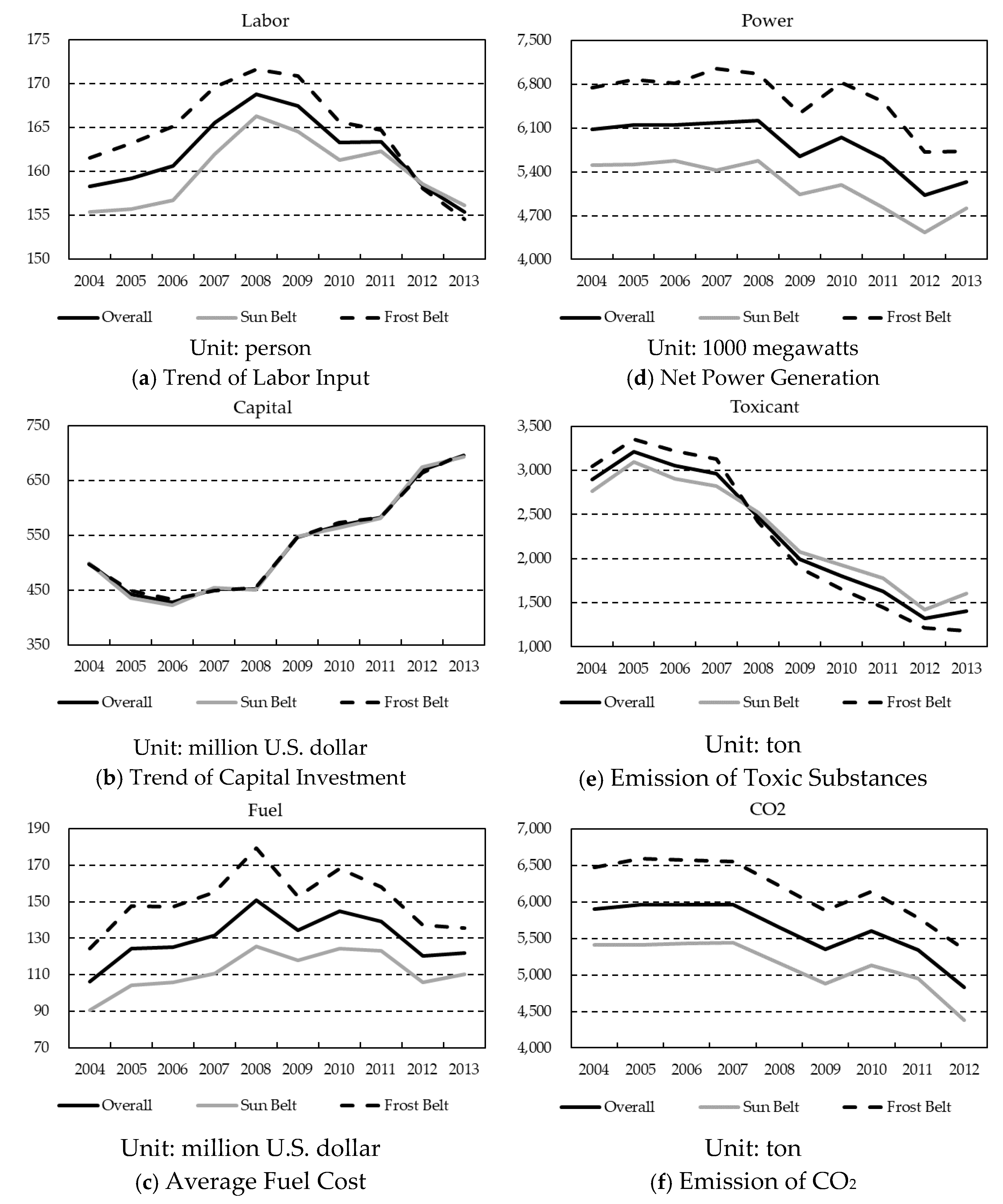
4.1. Overview of the Variables

Table 3. Descriptive statistics on inputs and outputs and tests on the difference between groups.

Variables	Overall	Sun Belt	Frost Belt	Diff. F Test (Sun Belt vs. Frost Belt) a
L	162.024	159.880	164.479	0.55
	(113.160)	(96.033)	(130.069)
K	533.44	532.20	534.85	0.014
	(414.20)	(443.41)	(378.36)
F	129.89	111.85	150.54	38.64	***
	(114.830)	(90.16)	(134.90)
P	5828.094	5189.99	6558.82	28.05	***
	(4749.74)	(4347.58)	(5077.91)
T	2275.12	2291.92	2255.89	0.048
	(2980.24)	(2897.32)	(3074.69)
C	5553.82	5089.85	6085.13	16.86	***
	(4435.40)	(4124.66)	(4713.98)
Plant Age	39.856	42.99	36.27	69.41	***
	(15.056)	(15.79)	(13.30)
Use of Natural Gas	0.25	0.21	0.30	14.91	***
	(0.44)	(0.41)	(0.46)
Coal Ratio	0.972	0.976	0.968	0.26
	(0.082)	(0.072)	(0.094)
Content of Sulfate	0.43	0.52	0.32	57.19	***
	(0.50)	(0.50)	(0.47)
Plant Scale	1.14	1.04	1.26	26.26	***
	(0.79)	(0.72)	(0.84)
Process Control	0.48	0.50	0.47	0.057
	(2.68)	(2.96)	(2.32)
Process Improvement	0.25	0.001	0.55	13.47	***
	(2.71)	(0.038)	(3.95)
Beginning Process Control	0.60	0.60	0.60	0.00
	(0.49)	(0.49)	(0.49)
Process Control Enhancement	0.40	0.40	0.40	0.00
	(0.49)	(0.49)	(0.49)

Notes: *** denote coefficient significance at the 1%, level, respectively. The figures in the parentheses are standard deviations. All the figures in this table are provided with two-digit significance. ^a: The ‘Diff. F test’ refers to the one-way ANOVA difference test for the Sun Belt and Frost Belt.

first lists the descriptive statistics of the input and output variables for the sample period, and also the results from testing the differences between the variables. The table shows several interesting points. First, when comparing the Sun Belt and Frost Belt, even though there is no significant difference between the average value of labor and capital, the Frost Belt obviously has higher fuel expenditure. Second, the two regions have a comparable scale on the output side, but the Frost Belt has a significantly higher desirable output with correspondingly higher CO₂ emissions. However, there is no notable difference in toxic emissions between the two regions. Third, on the input side, some differences between the two groups are significant. Among them, the Sun Belt has a higher plant age than the Frost Belt, indicating that power plants in the Frost Belt are newer and have more natural gas power generators. In addition, the two regions have similar ratios regarding coal-fired power generation, but the Sun Belt uses more sub-bituminous coal than the Frost Belt. Meanwhile, power plants in the Frost Belt tend to have a larger power capacity. In terms of voluntary emission reduction measures, there is no significant difference in process control between the two groups, but the Frost Belt has a greater process improvement. Overall, Table 3 indicates that power plants in the Sun Belt and Frost Belt have different characteristics. Nonetheless, the descriptive statistics alone cannot tell the differences between the groups in terms of environmental efficiency.

Figure 1 shows the trend of each variable during the sample period. The two groups appear to share a similar pattern. Figure 1a shows that the labor input has an upward trend before 2008, and a downward trend after. Figure 1b shows that capital investment in the Sun Belt and Frost Belt almost overlaps, and even more so after 2008, perhaps reflecting the impact of legislation on environmental protection. Table 1c examines the cost of fuel. It maintains a steady growth up to 2008, due to a moderately growing coal price. The cost of fuel has declined year by year since 2008, conceivably caused by the decrease in the natural gas price and the decline in overall power generation. Figure 1d depicts the trend of net power generation and highlights the continuous decrease after 2008. Figure 1e presents a downward trend of carbon dioxide emissions, possibly due to reduced power generation, increased technology, and equipment upgrades. For similar reasons, Figure 1f shows that emissions of toxic substances started to decrease in 2007.

4.2. Estimating Environmental Performance

The model estimation involved two levels: Group frontier and metafrontier.

Table 4. Group frontier and metafrontier: Maximum likelihood estimation.

Variables	Sun Belt frontier			Frost Belt frontier			Metafrontier
Constant	1.16	***	(0.45)	1.79	***	(0.30)	2.0037	***	(0.0818)
lnL	0.10		(0.18)	−0.43	***	(0.10)	−0.312	***	(0.025)
lnK	−0.25	**	(0.11)	−0.510	***	(0.053)	−0.471	***	(0.016)
lnE	−0.20	**	(0.10)	0.372	***	(0.073)	0.133	***	(0.021)
lnT’	−0.120	***	(0.047)	−0.102	***	(0.024)	−0.1041	***	(0.0061)
lnC’	−0.389	***	(0.062)	−0.403	***	(0.051)	−0.402	***	(0.013)
lnL2	−0.057		(0.041)	−0.033		(0.025)	−0.0587	***	(0.0067)
lnK2	−0.024		(0.026)	−0.0011		(0.0016)	−0.00312	***	(0.00061)
lnE2	−0.023		(0.024)	−0.0453	***	(0.0077)	−0.0298	***	(0.0027)
lnT’2	−0.0259	***	(0.0048)	−0.0069	***	(0.0011)	−0.00692	***	(0.00033
lnC’2	−0.0802	***	(0.0041)	−0.0826	***	(0.0016)	−0.08024	***	(0.00052)
lnL x lnK	0.0012		(0.0241)	0.025	**	(0.011)	0.0071	**	(0.0033)
lnL x lnE	−0.00030		(0.04051)	−0.139	***	(0.022)	−0.1286	***	(0.0054)
lnK x lnE	−0.050	**	(0.025)	−0.130	***	(0.014)	−0.0874	***	(0.0036)
lnT x lnC’	0.0412	***	(0.0062)	0.0169	***	(0.0031)	0.01733	***	(0.00082)
lnL x lnT’	0.00071		(0.01030)	−0.0155	***	(0.0061)	−0.0094	***	(0.0017)
lnK x lnT’	−0.0212	**	(0.0093)	−0.0025		(0.0047)	−0.0069	***	(0.0015)
lnE x lnT’	−0.0179	*	(0.0097)	−0.0038		(0.0045)	−0.0058	***	(0.0012)
lnL x lnC’	0.012		(0.023)	0.079	***	(0.014)	0.0776	***	(0.0034)
lnK x lnC’	0.052	***	(0.013)	0.0583	***	(0.0095)	0.0533	***	(0.0025)
lnE x lnT’	0.0534	***	(0.0096)	0.0765	***	(0.0046)	0.0721	***	(0.0013)
t	−0.162	***	(0.023)	−0.070	***	(0.013)	−0.0897	**	(0.0035)
t2	0.00082		(0.00113)	0.00031		(0.00072)	0.00091	***	(0.00023)
lnL x t	−0.0015		(0.0041)	0.0075	***	(0.0023)	0.00611	***	(0.00073)
lnK x t	0.0059	*	(0.0031)	0.0048	***	(0.0017)	0.00533	***	(0.00052)
lnE x t	−0.0448	***	(0.0057)	−0.0137	***	(0.0026)	−0.02364	***	(0.00083)
lnT’ x t	0.0013		(0.0014)	0.00243	***	(0.00081)	0.00254	***	(0.00032)
lnC’ x t	0.0191	***	(0.0031)	0.0019		(0.0015)	0.00580	***	(0.00054)
Plant Age	0.0065	***	(0.0011)	−0.0051	***	(0.0013)		-
Use of Natural Gas	0.019		(0.027)	−0.489	***	(0.043)		-
Coal Ratio	−0.952	***	(0.071)	−1.59	***	(0.13)		-
Content of Sulfate	−0.224	***	(0.042)	−0.228	***	(0.077)		-
Plant Scale	−0.415	***	(0.046)	−0.272	***	(0.021)		-
Process Control	−0.0073		(0.0168)	−0.0387	***	(0.0041)		-
Process Improvement	−1.079	***	(0.087)	−0.0084	***	(0.0015)		-
Beginning Process Control	-		-	-		-	0.139	***	(0.019)
Process Control Enhancement	-		-	-		-	0.234	***	(0.025)
δ	0.31	***	(0.12)	0.966	***	(0.062)	−1.4196	***	(0.1715)
σ2	0.0453		(0.0027)	0.0591	***	(0.0085)	0.0269	***	(0.0032)
γ	0.9336		(0.0085)	0.9849		(0.0031)	0.9929	***	(0.0013)
Adjusted R2	0.54			0.47			0.81
λ	325.91 ***						-

Notes: ***, **, and * denote coefficient significance at 1%, 5%, and 10%, respectively. The lnT’ and lnC’ in turn denote lnT/lnP and lnC/lnP. a: Log-likelihood ratio test; H₀: the frontiers of the Sun Belt and Frost Belt are identical; H₁: the frontiers of the Sun Belt and Frost Belt are distinct. The LR statistic is defined by λ = −2{ln[L(H₀)]−ln[L(H₁)]}, where the ln[L(H₀)] is the value of the log- likelihood function for the frontier estimated by pooling all the firms, while ln[L(H₁)] is the sum of the values of the log-likelihood functions for the two group frontiers. All the figures in this table are provided with two-digit significance. The figures in the parentheses are standard errors.

presents the results from estimating the group frontier of the Sun Belt and Frost Belt. There are several key points worth discussing. First, we conducted the heterogeneity test on the group frontiers. The λ value of the log-likelihood ratio test shows that the results from estimating the group frontier separately are significantly better than the pooled estimation, at the 1% level. This is consistent with our a priori judgement and the descriptive statistics that the Sun Belt and Frost Belt belong to two groups with different technology. Second, parameter estimates of the Sun Belt and Frost Belt frontier show that the undesirable output (T) and CO₂ have a negative effect on the distance function. This indicates that an increase of the undesirable output will increase the value of the distance function, leading to a reduction of environmental efficiency. Third, the γ values for the Sun Belt and Frost Belt are 0.9336 and 0.9849, respectively, indicating that the actual production points of both groups deviate from the technical frontier. That means 93.36% and 98.49% are due to production inefficiency, and only 6.64% and 1.51% can be attributed to random error. This empirical evidence supports the use of stochastic frontiers for the analysis.

The fourth point concerns the influence of factory age. For the Sun Belt group, as expected, factory age has a significant and positive contribution to inefficiency. This is consistent with Pollitt [71], Yang and Pollitt [70], and Wei et al. [41]. However, for the Frost Belt group, factory age has a negative influence on inefficiency. This finding may seem quite surprising at first. To find the answer, we used the average factory age of 36.26 from Table 3 to figure out retrospectively that the Frost Belt group adopted new equipment around 1976, six years after the policy requiring that newly built power plants must use low-pollution generators [31]. Therefore, we can infer that most of the power plants in the Frost Belt region have experienced one equipment upgrade. However, the new environmental technology may only increase the input cost without simultaneously increasing the output, causing inefficiency for factories located in the Frost Belt area. Fifth, those power plants that use natural gas to generate electricity tend to have lower inefficiency. Our findings for the Frost Belt group in Table 4 confirm this, and the results are also consistent with Sarica and Or [73] and See and Coelli [75]. Nevertheless, the findings for the Sun Belt group are insignificant.

The sixth issue concerns the coal-burning ratio. Results from both groups show that an increase in the proportion of coal burning can significantly reduce inefficiency. Seventh, the use of sub-bituminous coal can suppress inefficiency in both groups, indicating that cleaner coal can not only reduce environmental pollution, but it can also increase technical efficiency. This finding is consistent with Fleishman et al. [33]. Eighth, results from both the Sun Belt and Frost Belt show that increasing the power capacity can result in economies of scale and help reduce inefficiency [33,40,70]. Ninth, process control, a component of the implementation of voluntary emission reduction, reduces inefficiency for the Frost Belt group. There is no significant effect for the Sun Belt group. Finally, we find that process improvement reduces inefficiency for both the Sun Belt and Frost Belt.

Table 4 also reports the estimated results of the “Metafrontier”. The γ value is 0.9929, indicating that under the metafrontier, inefficiency accounts for 99.29% of the error. It is also interesting to find that parameter estimates of process control and process improvement over greenhouse gas are positive and significant at the 1% level. This implies that the enactment of legislation on environmentally conscious process control and process improvement has increased inefficiency.

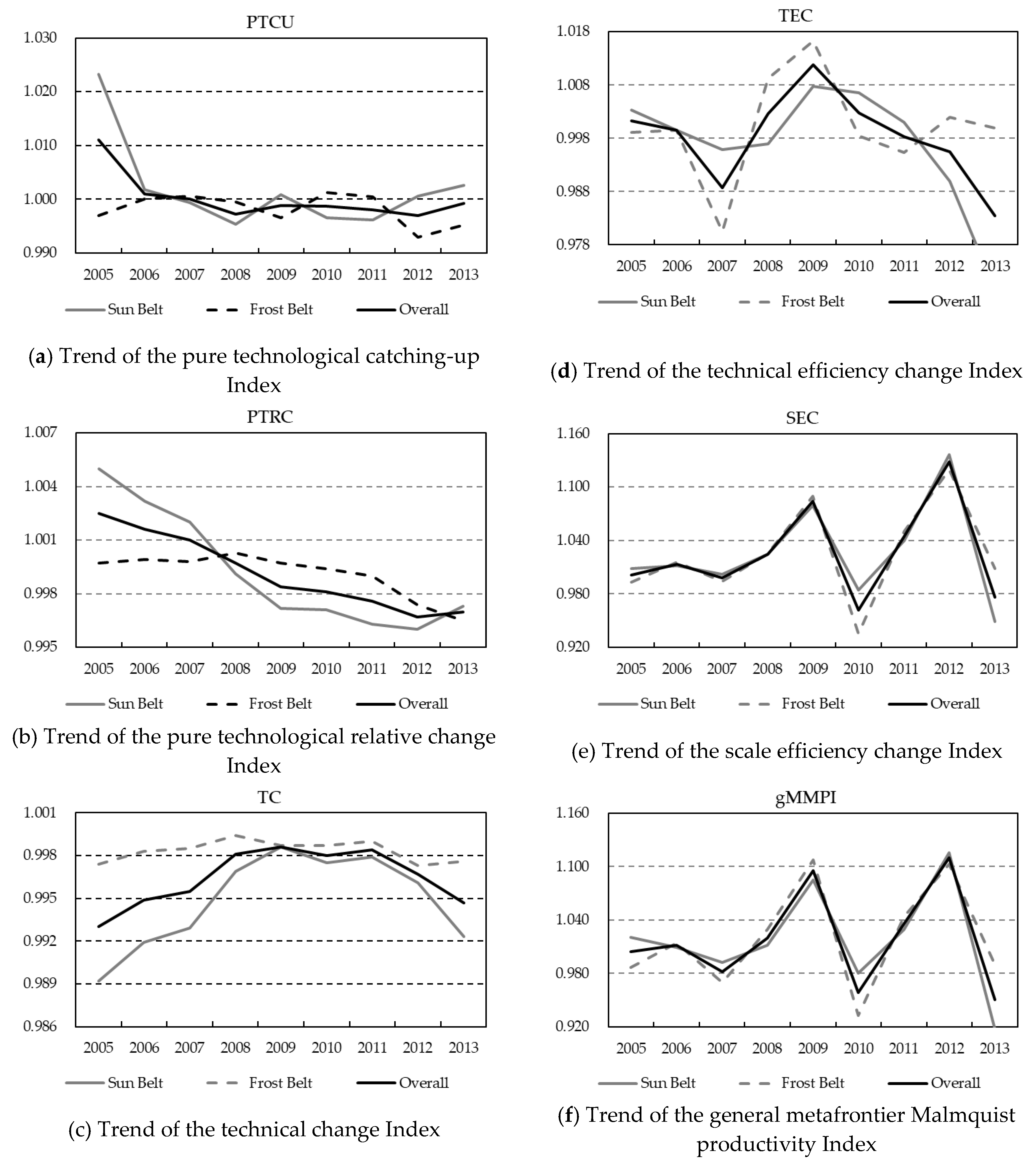
4.3. Measuring Environmental Performance

Table 5. Estimation of environment efficiency.

Group	Year	GTE a		TGR b		MTE c
		Mean	(Std. Dev.)	Mean	(Std. Dev.)	Mean	(Std. Dev.)
Sun Belt	2004	0.956	(0.049)	0.966	(0.052)	0.924	(0.065)
	2005	0.957	(0.008)	0.986	(0.026)	0.944	(0.025)
	2006	0.956	(0.007)	0.988	(0.028)	0.945	(0.027)
	2007	0.952	(0.012)	0.987	(0.033)	0.940	(0.034)
	2008	0.948	(0.015)	0.983	(0.037)	0.932	(0.040)
	2009	0.958	(0.013)	0.984	(0.035)	0.942	(0.039)
	2010	0.961	(0.020)	0.980	(0.030)	0.942	(0.036)
	2011	0.961	(0.020)	0.976	(0.031)	0.939	(0.038)
	2012	0.953	(0.016)	0.977	(0.047)	0.931	(0.050)
	2013	0.924	(0.018)	0.979	(0.130)	0.905	(0.129)
	Average	0.953	(0.018)	0.981	(0.045)	0.934	(0.048)
FrostBelt	2004	0.960	(0.017)	0.983	(0.027)	0.944	(0.032)
	2005	0.959	(0.020)	0.980	(0.041)	0.940	(0.046)
	2006	0.958	(0.018)	0.980	(0.043)	0.939	(0.047)
	2007	0.941	(0.016)	0.981	(0.094)	0.922	(0.093)
	2008	0.937	(0.016)	0.980	(0.062)	0.918	(0.063)
	2009	0.949	(0.026)	0.977	(0.064)	0.928	(0.071)
	2010	0.950	(0.014)	0.980	(0.063)	0.931	(0.062)
	2011	0.944	(0.013)	0.981	(0.077)	0.926	(0.077)
	2012	0.944	(0.020)	0.978	(0.069)	0.923	(0.070)
	2013	0.938	(0.028)	0.973	(0.072)	0.913	(0.076)
	Average	0.948	(0.019)	0.979	(0.061)	0.928	(0.064)
Overall	2004	0.958	(0.039)	0.974	(0.042)	0.933	(0.053)
	2005	0.958	(0.015)	0.983	(0.034)	0.942	(0.036)
	2006	0.957	(0.014)	0.984	(0.036)	0.942	(0.038)
	2007	0.947	(0.014)	0.984	(0.068)	0.932	(0.068)
	2008	0.943	(0.016)	0.982	(0.051)	0.926	(0.052)
	2009	0.954	(0.020)	0.981	(0.051)	0.935	(0.057)
	2010	0.956	(0.017)	0.980	(0.048)	0.937	(0.050)
	2011	0.954	(0.018)	0.979	(0.057)	0.933	(0.059)
	2012	0.948	(0.018)	0.977	(0.058)	0.927	(0.060)
	2013	0.930	(0.023)	0.976	(0.107)	0.908	(0.108)
	Average	0.950	(0.039)	0.980	(0.042)	0.932	(0.053)
Diff. F test (Sun Belt vs. Frost Belt) d				4.109	***	4.047	***

Notes: *** denote coefficient significance at the 1%, level, respectively. The ‘Std. Dev.’ in the column names is standard deviation. The figures in the parentheses are standard errors. ^d: The ‘Diff. F test’ refers to the one-way ANOVA difference test for the Sun Belt and Frost Belt. The full names of the acronyms are listed as follows: ^a: The ‘GTE’ is an acronym of the group technical efficiency. ^b: The ‘TGR’ is an acronym of the technical gap ratio. ^c: The ‘MTE’ is an acronym of the metafrontier technical efficiency.

reports the group technical efficiency, technology gap rate, and meta-technical efficiency obtained through estimating the group frontier and metafrontier. The table contains at least two important points. Overall, the meta-technical efficiency shows that fossil power plants have impressive environmental performance during the sample period, and all the efficiency scores are over the level of 0.9. Nonetheless, the dynamics are weakening year by year. On the one hand, the group efficiency of the power plants showed a downward trend. The Sun Belt group dropped from 0.956 in 2004 to 0.924 in 2013, indicating that the inefficiency increased from 4.4% to 7.6%. The Frost Belt group also decreased from 0.960 in 2004 to 0.938 in 2013, meaning the inefficiency increased from 4% to 6.2%. On the other hand, although the technology gap rate increased between 2004 and 2007, it has started to fall slightly since 2007 for both groups. This implies that since 2007, the gap between the plant actual technology and the best practice level is widening.

From the perspective of group comparison, the environmental efficiency of the Sun Belt group is slightly better than that of the Frost Belt. Table 5 shows that the meta-technical efficiency (MTE) of the Sun Belt is 0.934, indicating that under the existing conditions, there is a gap of 6.6% for the Sun Belt to raise its output level. The Frost Belt meta-technical efficiency (MTE) is 0.928, meaning the Frost Belt can potentially increase its output level by 7.2%. The result could have come from two sources. The first one is the technology gap rate (TGR). The technology gap rate of the Sun Belt is 0.981, showing that there is a 1.9% gap when compared to the best practice. The technology gap rate of the Frost Belt is 0.979, representing a gap of approximately 2.1%. The second source is the group technical efficiency. The group technical efficiency of the Sun Belt and Frost Belt is 0.953 and 0.948, respectively. This finding indicates that relative to the best practice, the inefficiency level is 4.7% for the Sun Belt and 5.5% for the Frost Belt. In term of environmental efficiency, we conclude that the Sun Belt group has done better than the Frost Belt group.

Knowing the estimation results thus far, we can now estimate the productivity index and its components.

Table 6. Estimation of environment productivity.

	Years	PTCU b	PTRC c	TC d	TEC e	SEC f	gMMPI a
Sun Belt	2004–2005	1.02320	1.00500	0.98920	1.00330	1.00840	1.02030
	2005–2006	1.00180	1.00320	0.99190	0.99950	1.01200	1.00930
	2006–2007	0.99940	1.00200	0.99290	0.99590	1.00170	0.99270
	2007–2008	0.99530	0.99910	0.99690	0.99700	1.02430	1.01170
	2008–2009	1.00090	0.99720	0.99860	1.00780	1.07930	1.08520
	2009–2010	0.99650	0.99710	0.99750	1.00650	0.98430	0.98020
	2010–2011	0.99610	0.99630	0.99790	1.00100	1.03950	1.02960
	2011–2012	1.00060	0.99600	0.99610	0.98990	1.13620	1.11560
	2012–2013	1.00260	0.99730	0.99230	0.96970	0.94930	0.91790
	Average	1.00180	0.99920	0.99480	0.99670	1.02610	1.01800
Frost Belt	2004–2005	0.99690	0.99970	0.99740	0.99910	0.99290	0.98720
	2005–2006	1.00000	0.99990	0.99830	0.99960	1.01570	1.01390
	2006–2007	1.00060	0.99980	0.99850	0.98050	0.99360	0.97030
	2007–2008	0.99950	1.00030	0.99940	1.00930	1.02560	1.02960
	2008–2009	0.99650	0.99970	0.99870	1.01630	1.08990	1.10730
	2009–2010	1.00120	0.99940	0.99870	0.99850	0.93530	0.93290
	2010–2011	1.00040	0.99900	0.99900	0.99530	1.05030	1.04410
	2011–2012	0.99300	0.99740	0.99730	1.00200	1.11980	1.10310
	2012–2013	0.99520	0.99650	0.99760	1.00000	1.00880	0.99030
	Average	0.99810	0.99910	0.99830	1.00010	1.02580	1.01990
Overall	2004–2005	1.01100	1.00250	0.99300	1.00130	1.00120	1.00490
	2005–2006	1.00100	1.00160	0.99490	0.99950	1.01370	1.01140
	2006–2007	1.00000	1.00100	0.99550	0.98870	0.99790	0.98220
	2007–2008	0.99720	0.99970	0.99810	1.00270	1.02490	1.02000
	2008–2009	0.99890	0.99840	0.99860	1.01180	1.08430	1.09560
	2009–2010	0.99870	0.99810	0.99800	1.00280	0.96190	0.95850
	2010–2011	0.99810	0.99760	0.99840	0.99830	1.04450	1.03630
	2011–2012	0.99700	0.99670	0.99670	0.99550	1.12860	1.10970
	2012–2013	0.99930	0.99700	0.99470	0.98340	0.97620	0.95070
	Average	1.00010	0.99920	0.99640	0.99820	1.02590	1.01880

Notes: The full names of the acronyms are listed as follows: ^a: The ‘gMMPI’ is an acronym of the generalized metafrontier Malmquist productivity index. ^b: The ‘PTCU’ is an acronym of pure technological catching-up. ^c: The ‘PTRC’ is an acronym of the pure technological relative change. ^d: The ‘TC’ is an acronym of the technical change. ^e: The ‘TEC’ is an acronym of the technical efficiency change. ^f: The ‘SEC’ is an acronym of the scale efficiency change.

shows that the overall average productivity of the U.S. fossil fuel power plants is on the rise, with the main source of contribution coming from the scale efficiency change. Table 6 reports that the generalized metafrontier Malmquist productivity index of all power plants is 1.0188, indicating an increase of 1.88% per year. Among them, the scale efficiency change is 1.0259, meaning that the production is approaching the most productive scale size at the speed of 2.59% per year. The impacts from other components are relatively minor. The value of the pure technological catching-up is 1.0001, which means the technical gap rate is converging toward the potential production level at an annual rate of 0.01%. Since the average value of the potential technological relative change, technical change, and technical efficiency change are all smaller than 1, and are 0.9992, 0.9964, and 0.9982, respectively, the current technical levels for the Sun Belt and Frost Belt are approaching the overall potential level at a decreasing rate. This was accompanied by a decline in efficiency and production technology improvement.

From the perspective of the group, the results are similar. The adjustment of scale efficiency drives the growth of the total factor productivity of the power plants while the impact of the remaining components is relatively trivial. For the Sun Belt group, the productivity is increasing at 1.8% annually as represented by the average generalized metafrontier Malmquist productivity index (gMMPI) of 1.0180. In the same time, the scale efficiency change growth index is 1.0261 on average, showing an annual growth rate of 2.61%. Since the average pure technological catching-up (PTCU) is 1.0018, the convergence rate of the technology gap ratio is merely 0.18% per year. In addition, pure technological catching-up, technical change, and technical efficiency change are less than 1, showing a slowing in the growth rate. The Frost Belt group has a generalized metafrontier Malmquist productivity index of 1.0199, which means productivity increases by an average of 1.99%. The scale efficiency change index averages 1.0258, representing an annual growth rate of approximately 2.58%. The value of the technical efficiency change is just 1.0001. The pure technological catching-up, potential technological relative change, and technical change all show a slight decline.

In terms of the trends, Figure 2 shows several interesting points. First, between 2005 and 2006, pure technological catching-up for all power plants experienced a significant decline, even though the technical gap was still slightly converging toward the potential level. Perhaps the trend was due to a bottleneck in technical development encountered by power plants during this period. The trend fell below 1 after 2007, indicating that the technical gap expanded slightly in the opposite direction. Second, the potential technological relative change had a downward trend, showing that the potential for the power plants to upgrade technology continued to decrease. This situation is more obvious for the Sun Belt group. Figure 2 shows that, between 2007 and 2008, the potential technological relative change of the Sun Belt had dropped significantly and was below that of the Frost Belt. This could be due to the fact that since 2007, the measures to control greenhouse gases have had a greater impact on the Sun Belt.

Third, Figure 2c shows that the technical change of the power industry declined significantly and was more severe for the Sun Belt group. An explanation could be that global environmental awareness exerted some influence. There were cases where mild recovery appeared before 2007. After that, the fallback resumed and was especially so for the Sun Belt than for the Frost Belt. Fourth, Figure 2d shows that the technical efficiency change trend has been declining over the years. After a small improvement between 2006 and 2008, it turned into a downward trend in 2009 again. In recent years, the deterioration of the efficiency of the Sun Belt is even more obvious. Fifth, Figure 2d reports changes of the scale efficiency index. The Sun Belt and Frost Belt appeared to share similar patterns, remaining stable until 2007 and then experienced sharp drops in 2008–2009 and 2011–2012. This reflects the fact that power plants make scale adjustments infrequently and eventfully.

5. Conclusions

This paper applied the hyperbolic distance function method and the stochastic metafrontier method to the estimation of the environmental efficiency of U.S. power plants. We took into account the influence of undesirable outputs, geographical locations, and policy impacts. We also computed the generalized metafrontier Malmquist productivity index to obtain insights into the changes of the index and its components. The results show that due to the greenhouse gas control policy, capital investment by fossil fuel power plants has increased year by year while the fuel input has been declining gradually. As a result, the emissions of toxic substances and carbon dioxide have decreased significantly, along with a decline in the power output. Taken together, the results of the productivity index show that between 2004 and 2013, on average, the productivity of the Sun Belt and Frost Belt power plants increased by two waves: First, in 2008, and again around 2011. After that, it quickly fell back and showed a downward trend, especially for the Sun Belt zone. Our analysis shows that the change in productivity is mainly affected by the change in scale efficiency. We believe the main reason for this lies in the fact that the Clean Air Act began to control and regulate greenhouse gases from 2007 onwards and also required the power plant industry to report greenhouse gas emissions.

This paper has far-reaching implications spanning from the academic to the political, as demonstrated by two logical inversions. First, economic development should inherently be environmentally sustainable rather than incompatible. The alternative is a type of growth that is nothing more than resource abuse. As the damage of pollution to the environment is irreversible, continuous, and cumulative, human beings are not supposed to mistake that pollution control would be at the expense of economic output. As we pursue higher living standards, we ought to resolve ourselves to do so not at the expense of our ecosystems but through the ingenuity that has made mankind the powerful force it is today. Second, life is enduring; life will find a way. Once we stop treating environmental responsibility as an option, economic activities, too, will find a way. Economic development and environmental sustainability are not mutually exclusive. In fact, they are best enjoyed together. Our history of pollution is unkind to the environment, and we simply cannot tolerate it as we move forward.

Due to the limited literature published during recent years, the analysis of this study reveals the facts of environmental productivity for fossil fuel power plants in the U.S. and the efficacy of related policies. Based on the empirical works and logical inversions, we assert that environmental protection regulations have an impact on power output. Nonetheless, the goal for sustainability should still hold true, and the implementation of relevant Environmental Protection Agency policies and the Clean Air Act should continue to be supported. This issue is economic in nature, but it is more than that. This is an issue about environmental integrity. It is an opportunity to demonstrate to future generations the bravery and responsibility we possess to fight selfishness across generations. With notice of the decline in productivity found in this paper, power plants may seek measures to relieve and support them with this inevitable trend and impressive challenge.

References

1. Mills-Knapp, S.; Traore, K.; Ericson, B.; Keith, J.; Hanrahan, D.; Caravanos, J. The World’s Worst Pollution Problems: Assessing Health Risks at Hazardous Waste Sites; Blacksmith Institute: New York, NY, USA, 2012. [Google Scholar]
2. Hart, S.L. Beyond Greening: Strategies for a Sustainable World. Harv. Bus. Rev. 1997, 75, 66–77. [Google Scholar]
3. Gao, H.; Yang, W.; Yang, Y.; Yuan, G. Analysis of the Air Quality and the Effect of Governance Policies in China’s Pearl River Delta, 2015–2018. Atmosphere 2019, 10, 412. [Google Scholar] [CrossRef] [Green Version]
4. Statistics, I.E.A. CO2 Emissions from Fuel Combustion Highlights; IEA: Paris, France, 2011; Available online: http://www.iea.org/co2highlights/co2highlights.pdf (accessed on 31 July 2014).
5. Environmental Protection Agency. 2012 Toxics Release Inventory National Analysis Overview 2014. Available online: http://www2.epa.gov/toxics-release-inventory-tri-program/2012-tri-national-analysis (accessed on 13 March 2015).
6. Sueyoshi, T.; Goto, M. Should the US Clean Air Act Include CO2 Emission Control? Examination by Data Envelopment Analysis. Energy Policy 2010, 38, 5902–5911. [Google Scholar] [CrossRef]
7. Kumar, S.; Managi, S. Sulfur Dioxide Allowances: Trading and Technological Progress. Ecol. Econ. 2010, 69, 623–631. [Google Scholar] [CrossRef]
8. Yang, W.; Yuan, G.; Han, J. Is China’s Air Pollution Control Policy Effective? Evidence from Yangtze River Delta Cities. J. Clean. Prod. 2019, 220, 110–133. [Google Scholar] [CrossRef]
9. Yang, W.; Li, L. Efficiency Evaluation of Industrial Waste Gas Control in China: A Study Based on Data Envelopment Analysis (DEA) Model. J. Clean. Prod. 2018, 179, 1–11. [Google Scholar] [CrossRef]
10. Yuan, G.; Yang, W. Evaluating China’s Air Pollution Control Policy with Extended AQI Indicator System: Example of the Beijing-Tianjin-Hebei Region. Sustainability 2019, 11, 939. [Google Scholar] [CrossRef] [Green Version]
11. Hu, H.; Jin, Q.; Kavan, P. A Study of Heavy Metal Pollution in China: Current Status, Pollution-Control Policies and Countermeasures. Sustainability 2014, 6, 5820–5838. [Google Scholar] [CrossRef] [Green Version]
12. Pettersson, M.; Söderholm, P. Industrial Pollution Control and Efficient Licensing Processes: The Case of Swedish Regulatory Design. Sustainability 2014, 6, 5401–5422. [Google Scholar] [CrossRef] [Green Version]
13. Zhang, N.; Kong, F.; Choi, Y.; Zhou, P. The Effect of Size-Control Policy on Unified Energy and Carbon Efficiency for Chinese Fossil Fuel Power Plants. Energy Policy 2014, 70, 193–200. [Google Scholar] [CrossRef]
14. Zhang, N.; Choi, Y. Total-Factor Carbon Emission Performance of Fossil Fuel Power Plants in China: A Metafrontier Non-Radial Malmquist Index Analysis. Energy Econ. 2013, 40, 549–559. [Google Scholar] [CrossRef]
15. Zhang, N.; Zhou, P.; Choi, Y. Energy Efficiency, CO2 Emission Performance and Technology Gaps in Fossil Fuel Electricity Generation in Korea: A Meta-Frontier Non-Radial Directional Distance Function Analysis. Energy Policy 2013, 56, 653–662. [Google Scholar] [CrossRef]
16. Sueyoshi, T.; Goto, M. DEA Radial Measurement for Environmental Assessment and Planning: Desirable Procedures to Evaluate Fossil Fuel Power Plants. Energy Policy 2012, 41, 422–432. [Google Scholar] [CrossRef]
17. Chung, Y.H.; Färe, R.; Grosskopf, S. Productivity and Undesirable Outputs: A Directional Distance Function Approach. J. Environ. Manag. 1997, 51, 229–240. [Google Scholar] [CrossRef] [Green Version]
18. Zhang, N.; Choi, Y. A Comparative Study of Dynamic Changes in CO2 Emission Performance of Fossil Fuel Power Plants in China and Korea. Energy Policy 2013, 62, 324–332. [Google Scholar] [CrossRef]
19. Sueyoshi, T.; Goto, M. Returns to Scale vs. Damages to Scale in Data Envelopment Analysis: An Impact of US Clean Air Act on Coal-Fired Power Plants. Omega 2013, 41, 164–175. [Google Scholar] [CrossRef]
20. Färe, R.; Grosskopf, S. New Directions: Efficiency and Productivity; Kluwer Academic Publishers: Boston, MA, USA, 2004. [Google Scholar]
21. Shephard, R.W. Theory of Cost and Production Functions; Princeton University Press: Princeton, NJ, USA, 1970. [Google Scholar]
22. Cuesta, R.A.; Zofio, J.L. Hyperbolic Efficiency and Parametric Distance Functions: With Application to Spanish Savings Banks. J. Prod. Anal. 2005, 24, 31–48. [Google Scholar] [CrossRef]
23. Cuesta, R.A.; Lovell, C.K.; Zofio, J.L. Environmental Efficiency Measurement with Translog Distance Functions: A Parametric Approach. Ecol. Econ. 2009, 68, 2232–2242. [Google Scholar] [CrossRef]
24. Crandall, R.W. Clean Air and Regional Protectionism. Brook. Rev. 1983, 2, 17–20. [Google Scholar] [CrossRef]
25. Färe, R.; Grosskopf, S.; Pasurka, C.A., Jr. Accounting for Air Pollution Emissions in Measures of State Manufacturing Productivity Growth. J. Reg. Sci. 2001, 41, 381–409. [Google Scholar] [CrossRef]
26. Färe, R.; Grosskopf, S.; Pasurka, C.A., Jr. Toxic Releases: An Environmental Performance Index for Coal-Fired Power Plants. Energy Econ. 2010, 32, 158–165. [Google Scholar] [CrossRef]
27. Färe, R.; Grosskopf, S.; Pasurka, C.A., Jr. Social Responsibility: US Power Plants 1985–1998. J. Prod. Anal. 2006, 26, 259–267. [Google Scholar] [CrossRef]
28. Battese, G.E.; Rao, D.P.; O’Donnell, C.J. A Metafrontier Production Function for Estimation of Technical Efficiencies and Technology Gaps for Firms Operating under Different Technologies. J. Prod. Anal. 2004, 21, 91–103. [Google Scholar] [CrossRef]
29. Huang, C.J.; Huang, T.H.; Liu, N.H. A New Approach to Estimating the Metafrontier Production Function Based on a Stochastic Frontier Framework. J. Prod. Anal. 2014, 42, 241–254. [Google Scholar] [CrossRef]
30. Environmental Protection Agency. Cleaner Power Plant 2015. Available online: https://archive.epa.gov/epa/cleanpowerplan/fact-sheet-overview-clean-power-plan.html (accessed on 29 April 2017).
31. Rubin, E.S.; Taylor, M.R.; Yeh, S.; Hounshell, D.A. Learning Curves for Environmental Technology and Their Importance for Climate Policy Analysis. Energy 2004, 29, 1551–1559. [Google Scholar] [CrossRef] [Green Version]
32. Adair, S.K.; Hoppock, D.C.; Monast, J.J. New Source Review and Coal Plant Efficiency Gains: How New and Forthcoming Air Regulations Affect Outcomes. Energy Policy 2014, 70, 183–192. [Google Scholar] [CrossRef]
33. Fleishman, R.; Alexander, R.; Bretschneider, S.; Popp, D. Does Regulation Stimulate Productivity? The Effect of Air Quality Policies on the Efficiency of US Power Plants. Energy Policy 2009, 37, 4574–4582. [Google Scholar] [CrossRef]
34. Klassen, R.; McLaughlin, C. The Impact of Environmental Management on Firm Performance. Manag. Sci. 1996, 42, 1199–1214. [Google Scholar] [CrossRef]
35. Keffer, C.; Shimp, R.; Lehni, M. Eco-Efficiency Indicators and Reporting; World Business Council for Sustainable Development (WBCSD): London, UK, 1999. [Google Scholar]
36. Verfaillie, H.A.; Bidwell, R. Measuring Eco-efficiency: A Guide to Reporting Company Performance. World Business Council for Sustainable Development (WBCSD). 2000. Available online: https://www.gdrc.org/sustbiz/measuring.pdf (accessed on 3 December 2019).
37. Färe, R.; Grosskopf, S.; Lovell, C.K.; Pasurka, C. Multilateral Productivity Comparisons When Some Outputs Are Undesirable: A Nonparametric Approach. Rev. Econ. Stat. 1989, 75, 90–98. [Google Scholar] [CrossRef]
38. Murty, M.N.; Kummer, S.; Dhavala, K.K. Measuring Environmental Efficiency of Industry: A Case Study of Thermal Power Generation in India. Environ. Resour. Econ. 2007, 38, 31–50. [Google Scholar] [CrossRef]
39. Khanna, M.; Kummer, S. Corporate Environmental Management and Environmental Efficiency. Environ. Resour. Econ. 2011, 50, 227–242. [Google Scholar] [CrossRef]
40. Lin, Y.Y.; Chen, P.Y.; Chen, C.C. Measuring the Environmental Efficiency of Countries: A Directional Distance Function Metafrontier Approach. J. Environ. Manag. 2013, 119, 134–142. [Google Scholar]
41. Wei, C.; Loschel, A.; Liu, B. An Empirical Analysis of the CO2 Shadow Price in Chinese Thermal Power Plant. Energy Econ. 2013, 40, 22–31. [Google Scholar] [CrossRef]
42. Dong, F.; Li, X.; Liu, X. Regional Carbon Emission Performance in China According to a Stochastic Frontier Model. Renew. Sustain. Energy Rev. 2013, 28, 525–530. [Google Scholar] [CrossRef]
43. Ramanathan, R. An Analysis of Energy Consumption and Carbon Dioxide Emissions in Countries of the Middle East and North Africa. Energy 2005, 30, 2831–2842. [Google Scholar] [CrossRef]
44. Färe, R.; Grosskopf, S.; Noh, D.W.; Weber, W.L. Characteristics of a Polluting Technology: Theory and Practice. J. Econom. 2005, 126, 469–492. [Google Scholar] [CrossRef]
45. Managi, S.; Kumar, S. Trade-Induced Technological Change: Analyzing Economic and Environmental Outcomes. Econ. Model. 2009, 26, 721–732. [Google Scholar] [CrossRef]
46. Yang, M.; Yang, F.X.; Chen, X.P. Effects of Substituting Energy with Capital on China’s Aggregated Energy and Environmental Efficiency. Energy Policy 2011, 39, 6065–6072. [Google Scholar] [CrossRef]
47. Lee, M. The Shadow Price of Substitutable Sulfur in the US Electric Power Plant: A Distance Function Approach. J. Environ. Manag. 2005, 77, 104–110. [Google Scholar] [CrossRef]
48. Mekaroonreung, M.; Johnson, A. Estimating Efficiency of U.S. Oil Refineries Under Varying Assumptions Regarding Disposability of Bad Outputs. Int. J. Energy Sect. Manag. 2009, 4, 356–398. [Google Scholar] [CrossRef] [Green Version]
49. Sueyoshi, T.; Goto, M. DEA Approach for Unified Efficiency Measurement: Assessment of Japanese Fossil Fuel Power Generation. Energy Econ. 2011, 33, 292–303. [Google Scholar] [CrossRef]
50. GAO, U. Environmental Protection: More Consistency Needed Among EPA Regions in Approach to Enforcement; General Accounting Office: Washington, DC, USA, 2000. [Google Scholar]
51. Zwickl, K.; Ash, M.; Boyce, J.K. Regional Variation in Environmental Inequality: Industrial Air Toxics Exposure in US Cities. Ecol. Econ. 2014, 107, 494–509. [Google Scholar] [CrossRef] [Green Version]
52. Lau, L.J.; Yotopoulos, P.A. The Meta-Production Function Approach to Technological Change in World Agriculture. J. Dev. Econ. 1989, 31, 241–269. [Google Scholar] [CrossRef]
53. Battese, G.E.; Rao, D.P. Technology Gap, Efficiency, and a Stochastic Metafrontier Function. Int. J. Bus. Econ. 2002, 1, 87–93. [Google Scholar]
54. Oh, D.H. A Metafrontier Approach for Measuring an Environmentally Sensitive Productivity Growth Index. Energy Econ. 2010, 32, 146–157. [Google Scholar] [CrossRef]
55. Chiu, C.R.; Liou, J.L.; Wu, P.I.; Fang, C.L. Decomposition of the Environmental Inefficiency of the Meta-Frontier with Undesirable Output. Energy Econ. 2012, 34, 1392–1399. [Google Scholar] [CrossRef]
56. Yaisawarng, S.; Klein, J.D. The Effects of Sulfur Dioxide Controls on Productivity Change in the US Electric Power Industry. Rev. Econ. Stat. 1994, 76, 447–460. [Google Scholar] [CrossRef]
57. Huang, T.H.; Chiang, D.L.; Tsai, C.M. Applying the New Metafrontier Directional Distance Function to Compare Banking Efficiencies in Central and Eastern European Countries. Econ. Model. 2015, 44, 188–199. [Google Scholar] [CrossRef]
58. Battese, G.E.; Coelli, T.J. A Model for Technical Inefficiency Effects in a Stochastic Frontier Production Function for Panel Data. Empir. Econ. 1995, 20, 325–332. [Google Scholar] [CrossRef] [Green Version]
59. Caves, D.W.; Christensen, L.R.; Diewert, W.E. The Economic Theory of Index Numbers and the Measurement of Input, Output, and Productivity. Econometrica 1982, 50, 1393–1414. [Google Scholar] [CrossRef]
60. Caves, D.W.; Christensen, L.R.; Diewert, W.E. Multilateral Comparisons of Output, Input, and Productivity Using Superlative Index Numbers. Econ. J. 1982, 92, 73–86. [Google Scholar] [CrossRef]
61. Färe, R.; Grosskopf, S.; Norris, M.; Zhang, Z. Productivity Growth, Technical Progress, and Efficiency Change in Industrialized Countries. Am. Econ. Rev. 1994, 84, 66–83. [Google Scholar]
62. Rao, D.S.P. Metafrontier Frameworks for the Study on Firm-Level Efficiencies and Technology Gaps. In Proceedings of the 2006 Productivity and Efficiency Seminar, Taipei, Taiwan, 10 March 2006. [Google Scholar]
63. Campisi, D.; Mancuso, P.; Mastrodonato, S.; Morea, D. Efficiency Assessment of Knowledge Intensive Business Services Industry in Italy: Data Envelopment Analysis (DEA) and Financial Ratio Analysis. Meas. Bus. Excell. 2019, 23, 484–495. [Google Scholar] [CrossRef]
64. Diewert, W.E. Exact and Superlative Index Numbers. J. Econom. 1976, 4, 115–145. [Google Scholar] [CrossRef]
65. Färe, R.; Primont, D. Measuring the Efficiency of Multiunit Banking: An Activity Analysis Approach. J. Bank. Financ. 1993, 17, 539–544. [Google Scholar] [CrossRef]
66. Lovell, C.K.; Travers, P.; Richardson, S.; Wood, L. Resources and Functionings: A New View of Inequality in Australia. In Models and Measurement of Welfare and Inequality; Springer: Heidelberg/Berlin, Germany, 1994; pp. 787–807. [Google Scholar]
67. Färe, R.; Grosskopf, S.; Pasurka, C.A., Jr. Environmental Production Functions and Environment Directional Distance Functions. Energy 2007, 32, 1055–1066. [Google Scholar] [CrossRef]
68. Sueyoshi, T.; Goto, M.; Sugiyama, M. DEA Window Analysis for Environmental Assessment in a Dynamic Time Shift: Performance Assessment of U.S. Coal-Fired Power Plants. Energy Econ. 2013, 40, 845–857. [Google Scholar] [CrossRef]
69. Färe, R.; Grosskopf, S.; Pasurka, C.A., Jr. Potential Gains from Trading Bad Outputs: The Case of US Electric Power Plants. Resour. Energy Econ. 2014, 36, 99–112. [Google Scholar] [CrossRef]
70. Yang, H.; Pollitt, M. Incorporating both Undesirable Outputs and Uncontrollable Variables into DEA: The Performance of Chinese Coal-Fired Power Plants. Eur. J. Oper. Res. 2009, 197, 1095–1105. [Google Scholar] [CrossRef] [Green Version]
71. Pollitt, M.G. Ownership and Efficiency in Nuclear Power Production. Oxf. Econ. Pap. 1996, 48, 342–360. [Google Scholar] [CrossRef]
72. Chang, D.S.; Chen, Y.T.; Chen, W.D. The Exogenous Factors Affecting the Cost Efficiency of Power Generation. Energy Policy 2009, 37, 5540–5545. [Google Scholar] [CrossRef]
73. Sarıca, K.; Or, I. Efficiency Assessment of Turkish Power Plants Using Data Envelopment Analysis. Energy 2007, 32, 1484–1499. [Google Scholar] [CrossRef]
74. Lam, P.L.; Shiu, A. A Data Envelopment Analysis of the Efficiency of China’s Thermal Power Generation. Util. Policy 2001, 10, 75–83. [Google Scholar] [CrossRef]
75. See, K.F.; Coelli, T. An Analysis of Factors That Influence the Technical Efficiency of Malaysian Thermal Power Plants. Energy Econ. 2012, 34, 677–685. [Google Scholar] [CrossRef]
Figure 1. Input and output trends for U.S. fossil fuel power plants.
Sustainability 11 06907 g001
Figure 2. The potential technological relative change of the Sun Belt and that of the Frost Belt between 2007 and 2008. Notes: (a): The ‘gMMPI’ is an acronym of the generalized metafrontier Malmquist productivity index; (b): The ‘PTCU’ is an acronym of pure technological catching-up; (c): The ‘PTRC’ is an acronym of the pure technological relative change; (d): The ‘TC’ is an acronym of the technical change; (e): The ‘TEC’ is an acronym of the technical efficiency change; (f): The ‘SEC’ is an acronym of the scale efficiency change.
Sustainability 11 06907 g002