Risk Aversion Based Inexact Stochastic Dynamic Programming Approach for Water Resources Management Planning under Uncertainty

Abstract

In this study, a dual interval robust stochastic dynamic programming (DIRSDP) method is developed for planning water resources management systems under uncertainty. As an extension of the existing interval stochastic dynamic programming (ISDP) method, DIRSDP can deal with two-stage stochastic programming (TSP)-based planning problems associated with dynamic features, input uncertainties, and multistage concerns. Compared with other optimization methods dealing with uncertainties, the developed DIRSDP method has advantages in addressing uncertainties with complex presentations and reflecting decision makers’ risk-aversion attitudes within its optimization process. Parameters in the DIRSDP model can be represented as probability distributions as well as single and/or dual intervals. Decision makers’ risk-aversion attitudes can be reflected through restricting the deviation of the recourse costs to a tolerance level. Water-allocation plans can then be developed based on the analysis of tradeoffs between the system benefit and solution robustness. The developed method is applied to a case of water resources management planning. The solutions are reasonable, indicating applicability of the developed methodology.

1. Introduction

Controversial and conflict-laden water allocation issues between competing water users (e.g., municipal, industrial, and agricultural) have challenged water resource managers for many decades. An imbalance between increasing consumption from the users and decreasing acquisition of water resources is one of major challenges [1]. Such an imbalance will be exacerbated by climate change, population growth, urbanization, environmental contamination, technology development, and other impact factors. These impacts introduce uncertainty into water resources management decision making, leading to potential risks associated with economic losses and eco-environment degradation and thereby moving backwards sustainable development [2]. Therefore, effective methods for water resources management planning are desired in order to balance water demand and supply under uncertainty as well as balance economic return and environmental safe considering risk management [3,4,5,6,7,8].

Previously, two-stage stochastic programming (TSP) was reported as an effective tool for water resources planning under uncertainty [9,10,11,12,13,14,15,16,17,18]. The TSP methods reported are characterized by two essential features: the uncertainty (i.e., random river flows) is but not only expressed with a certain probabilistic distribution and the sequence of decisions. The local authority has to determine first, before the uncertain water availability is revealed, how much water the multiple competing users can expect (e.g., water allocation targets) for their various activities and development plans with an objective to maximize their net benefits. After the random water availability is realized, the authority might correct the preceding decisions at the second-stage due to water shortage, where the users might take recourse actions to obtain water from expensive alternatives or curtail their development plans. The second-stage decisions made will result in economic penalties (i.e., increased costs, economic losses, or negative consequences), denoting a reduction of the net benefit resulting from the first-stage decisions made [19]. Ji, L. et al. [16] developed an inexact TSP modelfor supporting regional water resource allocation management under uncertainties. The research handled the uncertainties of future water demand through generating a set of representative scenarios and analyzed different scenarios to discuss their effects on the water distribution patterns, water shortages, total benefits, and system cost. Khosrojerdi, T. et al. [18] developed optimal allocation strategies of water resources using a TSP method with interval and fuzzy parameters. In the abovementioned TSP approaches, the total expected value of the second-stage costs (e.g., economic penalties or recourse costs) is measured without considering and controlling the variabilities of the costs under different possible water-delivery scenarios. An unacceptably high second-stage cost might be incurred from water shortage, leading to a system-disruption risk, while the total expected second-stage cost over all possible scenarios remains relatively low. Accordingly, robust stochastic programming (RSP), as an extension of TSP, was developed to control the variabilities of the second-stage costs. A number of related studies have been reported [20,21,22,23,24]. For example, Mulvey, J.M. et al. [25] discussed a measure of the variability and introduced the concept of robustness. Ahmed, S. et al. [20] introduced a concept of upper partial mean (UPM) as a new measure of the variability of the cost.

Although TSP-related methods can assist in developing decision plans in an uncertain environment, they could not adequately support sequential decisions in long-term water resources planning problems. Such problems with stochastic and dynamic features are often tackled through stochastic dynamic programming (SDP) methods [26,27,28,29,30,31,32,33]. Most of the previous SDP methods are effective for state problems with dynamic and sequential structures but are limited for providing recourse actions in order to minimize the expected costs or maximize the expected net system benefits over the whole states [1]. To address this, a number of TSP-based SDP researches were reported for dealing with problems where recourse decisions are desired, dynamic variations of system conditions are to be reflected and/or the available data information cannot be expressed with precision [34,35,36,37,38,39]. For example, Luo, B. et al. [36] developed an interval stochastic dynamic programming model (ISDP) with embedded TSP submodels and applied it to a long-term water resources planning problem. ISDP can reflect dynamic complexities and uncertainties (expressed as probability distributions and intervals) through communicating them into simplified interval TSP submodels within a dynamic linear optimization framework.

However, some deficiencies could exist in TSP-based ISDP that limit its application. For example, there is a chance that the second-stage costs, resulting from high water-allocation targets determined at the first-stage and thereafter insufficient supplies delivered, may be unacceptably high and lead to a high system-disruption risk. On the other hand, deterministic values for lower and upper bounds of the input intervals may be unavailable. Normally, a single interval (a, b) has deterministic bounds a and b. If these bounds cannot be expressed as crisp values (i.e., they can only be quantified as distribution and/or membership functions), intervals (a, c) and (d, b) would be used to quantify the two bounds; this leads to dual uncertainties. Thus, a concept of dual interval (i.e.,((a, c), (d, b))) can be proposed [40,41].

Therefore, the aim of this study is to develop a dual interval robust stochastic dynamic programming (DIRSDP) approach for water resources management planning. Figure 1 shows the methodological framework of DIRSDP. DIRSDP is an extension of the existing interval stochastic dynamic programming (ISDP), where the concept of dual interval and upper partial mean measure (a robust analysis technique) are introduced into the ISDP to account for system complexities and risks. The developed method can deal with system uncertainties expressed as probability distributions and single/dual intervals, and reflect system dynamics and multistage decision concerns, as well as reflect subjective risk-aversion attitudes. Additionally, it can help decision-makers to identify desired management plans with risk control. To demonstrate applicability of the proposed method, DIRDSP will be applied to a case of water resources management planning. The solutions are analyzed to identify significant factors that affect the system’s performance and to gain insights into the tradeoffs between environmental and economic objectives.

2. Modeling Formulation

Consider the planning for a water resources system under uncertainty (i.e., random water availability). Multiple users (e.g., municipal, industrial, and agricultural) extract water from the same water body (e.g., lake, reservoir, and river) over a planning horizon of T time periods. In each planning period, the users will expand their activities (e.g., conducting municipal, industrial or irrigation infrastructures) according to their demands with an objective to maximize their net benefits. They are determined by random water availability. When water demand of a user is high, it would lead to a raised net benefit if the promised water is delivered; however, it would incur penalties (including extra costs or economic losses) if the expected water is not delivered. On the contrary, when the demand is low, it would result in reduced net benefits (with a decreased risk of water shortage) and, in addition, would incur wastage of resources when the available water is high. Thus, decisions of each user should be properly made in each planning period so that the expected value of net-system benefit over the entire planning period can be maximized.

Such a long-term water resources system planning problem can be formulated as an interval stochastic dynamic programming (ISDP) model. In each planning stage, decisions of capacity expansion based on water demands at a stage will influence water-allocation targets at the beginning of the next stage. Meanwhile, the allocation targets at the end of each time period will depend solely on the entering state variables and the decisions made at that stage; they are independent of decisions made at the previous stages [36]. To effectively reflect the system’s uncertainty and dynamic features, an inexact multistage optimization problem can be formulated with an objective of maximizing the expected net system benefit. Assume discrete distributions for the random parameters to avoid complicated computational requirements, thus, a deterministic equivalent formulation for ISDP can be expressed as follows (assuming zero initial capacities and stage values without loss of generality) [36,42]:

$$f_t^{\pm }=\underset{k\in N,t=1,\dots T}{\max }\left\{\left({\displaystyle \sum }_{i=1}^m{B}_{ti}^{\pm }{x}_{tik}-{\displaystyle \sum }_{i=1}^m{\displaystyle \sum }_{j=1}^n{p}_{tj}{C}_{ti}^{\pm }{y}_{tijk}^{\pm }\right)+f_{t-1}^{\pm }\left(x_{t-1i},y_{t-1ij}^{\pm },w_{t-1ik}\right)\right\}$$

(1)

$$f_0\left(x_{0i},y_{0ij},w_{0i}\right)=0$$

(2)

subject to:

$${\sum }_{i=1}^m\left(x_{tik}-y_{tijk}^{\pm }\right)\le q_{tj}^{\pm },\forall t,j;k\in N,$$

(3)

$$k{w}_{tik}\le x_{tik}-x_{t-1i}\le \left(k+1\right)w_{tik},\forall t,i;k\in N,$$

(4)

$$0\le y_{tijk}^{\pm }\le x_{tik},\forall t,i;k\in N,$$

(5)

$$x_{0i}=d_{1i},\forall i$$

(6)

where $B_{ti}^{\pm }$ is the net benefit per unit of water allocated to user i in stage t; $C_{ti}^{\pm }$ is the reduction of net benefit per unit of water not delivered to user i in stage t ($C_{ti}^{\pm }$ > $B_{ti}^{\pm }$); d_1i is the minimum water demand in stage 1 to user i; $f_t^{\pm }$ is the net-system benefit over the entire planning horizon and $f_0$ is the zero initial stage value; k is the expansion option of water demand in each stage t; $w_{tik}$ denotes the amount of expanded water to user i in stage t under an expansion option k; $x_{tik}$ are state variables, denoting the water-allocation target to user i (i = 1, …, m) in stage t on a given expansion option k (k = 1, …, k); $y_{tijk}^{\pm }$ is the amount by which water-allocation target $x_{tik}$ is not met in stage t when total available water is $q_{tj}$ with probability level $p_{tj}$ under a given expansion option k in stage t; and $x_{t-1i}$ and $y_{t-1ij}^{\pm }$ are fixed water-allocation targets and the amounts of water shortage in stage t − 1 under an expansion option k. The objective of Model (1)–(6) is to maximize $f_T^{\pm }$ over the entire planning horizon, where constraints in (3) are related to water availability, ensuring that water consumption of the system should be less than total water availability in each planning stage; constraints in (4) are related to state transformations enforcing the dependency of each user’s water-allocation target in stage t on the user’s expansion options in that stage, as well as on the water-allocation target in stage t − 1; constraints in (5) are related to allowable water allocation, guaranteeing that the water-allocation target of each user in each stage is greater than the water shortage; constraints in (6) reflect the initial minimum water demand for each user.

Model (1)–(6) is a stochastic dynamic linear program. In each planning stage, once an expansion option is chosen, a decision regarding water-allocation targets needs to be made before the realization of uncertain water availability; then, a recourse action can be taken after such uncertainties are presented to mitigate that losses occurred due to water shortage. Such a problem can be analyzed through interval two-stage stochastic programming (ITSP). Thus, Model (1)–(6) can be solved by a dynamic linear program with embedded ITSP sub-problems (Model (7)–(11)), which can be developed as follows [36]:

$$Max h_{tk}^{\pm }=\left(x_{tik},y_{tijk}^{\pm },w_{tik},k\right)={\displaystyle \sum }_{i=1}^m{B}_{ti}^{\pm }{x}_{tik}-{\displaystyle \sum }_{i=1}^m{\displaystyle \sum }_{j=1}^n{p}_{tj}{C}_{ti}^{\pm }{y}_{tijk}^{\pm }$$

(7)

subject to:

$${\sum }_{i=1}^m\left(x_{tik}-y_{tijk}^{\pm }\right)\le q_{tj}^{\pm },\forall t,j;k\in N,$$

(8)

$$k{w}_{tik}\le x_{tik}-x_{t-1i}^{*}\le \left(k+1\right)w_{tik},\forall t,i;k\in N,$$

(9)

$$0\le y_{tijk}^{\pm }\le x_{tik},\forall t,i;k\in N,$$

(10)

$$x_{0i}=d_{1i},\forall i$$

(11)

where $x_{t-1i}^{*}$ is the optimized water-allocation targets of user i in stage t − 1 under different expansion options, and $x_{0i}^{*}=d_{1i}$; $h_{tk}^{\pm }$ is the system benefit in stage (t). Such an ITSP sub-problem should be solved in each stage (t) to determine state variables ($x_{tik}$) in the hierarchy tree of the dynamic problem (1); then, a backward recourse can be taken to determine the optimal expansion options (k) in all planning stages so that the optimum of Model (1)–(6) can be obtained.

However, the before-mentioned ITSP sub-problem is based on an assumption that decision makers are risk-neutral with measuring the expected value of the second-stage costs and without controlling the degree of variability of the costs. Such an assumption might lead to an unacceptably high cost incurred from water shortage. To address this, a measure of the deviation is needed to quantify the variability of the recourse costs. Through limiting the deviation of the recourse cost to a tolerance level, the degree of variability of the cost can be controlled and the risk-aversion from the decision makers can then be reflected. Such a measure can be formulated as follows [43] (Equation (12)):

$$v\left(y_{ti1k},y_{ti2k},\dots y_{tijk}\right)\le \epsilon ,$$

(12)

where $\epsilon$ is a given tolerance level for the variability ($v\left(y_{ti1k},y_{ti2k},\dots ,y_{tijk}\right)$). Usually, as a symmetric risk measure, variance is the natural choice of the variability metric, which can penalize cost both above and below the expected recourse cost. However, it may cause the inclusion of nonlinearities into the formulation, leading to computational difficulties. Moreover, for water resources management problems, water shortages will incur penalties (recourse cost), while excess water should not be penalized. Thus, according to Ahmed, S. et al. [20], the upper partial mean (UPM) as an asymmetric measure of the variability of the recourse costs can be proposed as follows (Equations (13) and (14)):

$${\overline{\Delta }}_t\left(y_{ti1k},y_{ti2k},\dots y_{tijk}\right)={\displaystyle \sum }_{j=1}^n{p}_{tj}{\Delta }_{tj}\left(y_{ti1k},y_{ti2k},\dots y_{tijk}\right),$$

(13)

$${\Delta }_{tj}\left(y_{ti1k}, y_{ti2k},\dots y_{tijk}\right)=max\left\{C_{ti}{y}_{tijk}-{\displaystyle \sum }_{j=1}^n{p}_{tj}{C}_{ti}{y}_{tijk},0\right\}$$

(14)

In each planning stage, for scenario j (j = 1, 2, …, n), ${\Delta }_{tj}$ is the positive deviation of the cost from the expected recourse cost; in definition, ${\overline{\Delta }}_t$ is the expected cost of the positive deviations over all scenarios. UPM can be used as the measure of variance in the restricted recourse formulations (through linear constraints) by introducing additional variables (${\Delta }_{tj}$) as follows (Equation (15)):

$${\displaystyle \sum }_{j=1}^n{p}_{tj}{\Delta }_{tj}\le {\epsilon }_t$$

(15)

Introducing (15) to the above TSP framework, a TSP submodel with restricted recourse can be obtained. Mulvey, J.M. et al. [25] named such a modeling methodology as robust stochastic programming (RSP) because the deviation of the recourse costs was limited (close to the expected value over all possible scenarios) and the resulting solutions would not be significantly sensitive to the variations of random events [13].Thus, one potential extension of Model (1)–(6) would be to integrate interval-parameter RSP into a dynamic linear programming framework. This leads to an interval robust stochastic dynamic programming (RSDP) model as follows:

$$f_t^{\pm }=\underset{k\in N,t=1,\dots T}{\max }\left\{\left({\displaystyle \sum }_{i=1}^m{B}_{ti}^{\pm }{x}_{tik}-{\displaystyle \sum }_{i=1}^m{\displaystyle \sum }_{j=1}^n{p}_{tj}{C}_{ti}^{\pm }{y}_{tijk}^{\pm }\right)+f_{t-1}^{\pm }\left(x_{t-1i},y_{t-1ij}^{\pm },w_{t-1ik}\right)\right\}$$

(16)

$$f_0\left(x_{0i}, y_{0ij},w_{0i}\right)=0$$

(17)

subject to:

constraints (1)–(6)

$${\displaystyle \sum }_{j=1}^n{p}_{tj}{\Delta }_{tj}^{\pm }\le {\epsilon }_t^{\pm }$$

(18)

where $B_{ti}^{\pm }$, $C_{ti}^{\pm }$, $y_{tijk}^{\pm }$, $q_{tj}^{\pm }$, ${\Delta }_{tj}^{\pm }$, ${\epsilon }_t^{\pm }$, and $f_t^{\pm }$ are interval parameters or variables. Here, an interval is defined as a real number with known lower and upper bounds but unknown distribution information [44,45], where values of the bounds are deterministic.

However, dual uncertainties may exist when the available information for the boundaries of interval parameters cannot be acquired as deterministic values. For example, the reservoir outflows ($q_{tj}^{\pm }$) in Model (16)–(18) are expressed as intervals ((a₁, b₁), (a₂, b₂), (a₃, b₃)) with deterministic boundaries (a₁, a₂, a₃, b₁, b₂, b₃). Nevertheless, the lower and upper bounds of the intervals may not be known with certainty, leading to dual uncertainties. Thus, the concept of a dual interval (i.e., ((a₁, c₁), (d₁, b₁)), ((a₂, c₂), (d₂, b₂)), ((a₃, c₃), (d₃, b₃))) is proposed to reflect such dual uncertainties. With uncertain boundaries, an infinite number of intervals (single) derived from each dual interval could exist. For example, the lower and upper bounds of a dual interval ((a₁, c₁), (d₁, b₁)) may be valued as intervals (a₁, c₁) and (d₁, b₁), respectively. Then, the lower bound would take any value between a₁ and c₁, and the upper one between d₁ and b₁. Therefore, there would be infinite single intervals derived from this dual interval. When the reservoir outflows are expressed as dual intervals ((a₁, c₁), (d₁, b₁)), ((a₂, c₂), (d₂, b₂)), and ((a₃, c₃), (d₃, b₃)) (each with a probability of occurrence), complexities will then exist. The difference between single and dual intervals for the reservoir outflows can be visualized in Figure 2. Joslyn, C. [41] proposed a method to simply simulate a dual interval ((a, c), (d, b)) in a class of random intervals (interval-valued random variables). According to the available information, ten types of potential conditions can be derived from combinations of four endpoints (a, b, c, and d) of the dual interval (Figure 3 and Figure 4). Each of them is a collection of intervals with corresponding probabilities (e.g., random intervals). For example, when a and b (i.e., outliers of a dual interval) are considered to be more reliable than c and d, the interval can be simulated by random intervals (a, d), (a, b) and (c, b) with each having an identical probability of 0.33 [40]. According to Langewisch, A.T. et al. [46], the mean value of a random interval is (0.67a + 0.33c, 0.33d + 0.67b). The bounds for the mean have a general form (Equations (19) and (20)):

$$E^{-}={\displaystyle \sum }_{l=1}^l{m}_l{q}_l^{-}$$

(19)

$$E^{+}={\displaystyle \sum }_{l=1}^l{m}_l{q}_l^{+}$$

(20)

where $E^{-}$ and $E^{+}$ are bounds for the mean of the random intervals, m_l is assigned probability, and $q_l^{-}$ and $q_l^{+}$ are lower and upper bounds of each interval, respectively (Figure 5). Thus, if $q_{tj}^{\pm }$ in Model (16)–(18) are expressed as dual intervals, they can be simulated by a class of random intervals based on the available information of their endpoints.

Considering the dual uncertainties (in reservoir outflows) in Model (16)–(18), a dual interval robust stochastic dynamic programming (DIRSDP) model can be developed as follows:

$$f_t^{\pm }=\underset{k\in N,t=1,\dots T}{\max }\left\{\left({\displaystyle \sum }_{i=1}^m{B}_{ti}^{\pm }{x}_{tik}-{\displaystyle \sum }_{i=1}^m{\displaystyle \sum }_{j=1}^n{p}_{tj}{C}_{ti}^{\pm }{y}_{tijk}^{\pm }\right)+f_{t-1}^{\pm }\left(x_{t-1i},y_{t-1ij}^{\pm },w_{t-1ik}\right)\right\}$$

(21)

$$f_0\left(x_{0i},y_{0ij},w_{0i}\right)=0$$

(22)

subject to:

$${\sum }_{i=1}^m\left(x_{tik}-y_{tijk}^{\pm }\right)\le {\left[q_{tj}^{\pm }\right]}^{\pm },\forall t,j;k\in N,$$

(23)

$$k{w}_{tik}\le x_{tik}-x_{t-1i}\le \left(k+1\right)w_{tik},\forall t,i;k\in N,$$

(24)

$$0\le y_{tijk}^{\pm }\le x_{tik},\forall t,i;k\in N,$$

(25)

$$x_{0i}=d_{1i},\forall i$$

(26)

$${\displaystyle \sum }_{j=1}^n{p}_{tj}{\Delta }_{tj}^{\pm }\le {\epsilon }_t^{\pm }$$

(27)

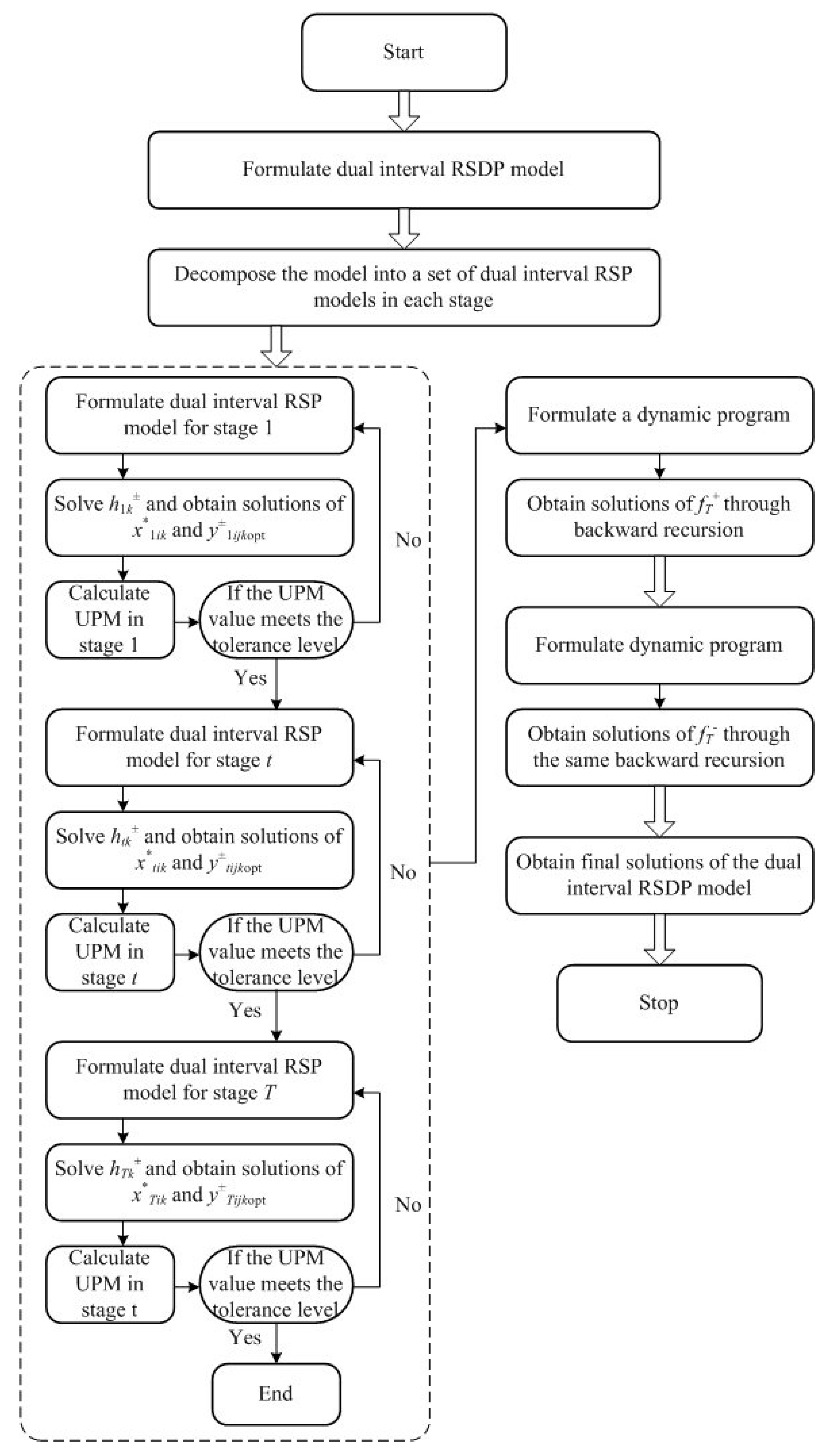
where ${\left[q_{tj}^{\pm }\right]}^{\pm }$ denotes dual interval flows. Thus, under a given expansion option, Model (21)–(27) can be decomposed into many stages; for each stage, a dual interval RSP sub-problem can be formulated. In order to obtain the solution of Model (21)–(27), the dual interval RSP sub-problem for each stage should firstly be solved. Figure 6 illustrates a general flowchart of the solution for Model (21)–(27), and the detailed solution approach is presented in the next section.

3. Solution Method

In Model (21)–(27), when water-allocation targets ($x_{t-1ik}$) in stage t − 1 are determined under given expansion options, $x_{tik}$ in stage t under option k can be approached by the following dual interval robust stochastic programming (DIRSP) submodel:

$$Max h_{tk}^{\pm }=\left(x_{tik},y_{tijk}^{\pm },w_{tik},k\right)={\displaystyle \sum }_{i=1}^m{B}_{ti}^{\pm }{x}_{tik}-{\displaystyle \sum }_{i=1}^m{\displaystyle \sum }_{j=1}^n{p}_{tj}{C}_{ti}^{\pm }{y}_{tijk}^{\pm }$$

(28)

subject to:

$${\sum }_{i=1}^m\left(x_{tik}-y_{tijk}^{\pm }\right)\le {\left[q_{tj}^{\pm }\right]}^{\pm },\forall t,j;k\in N,$$

(29)

$$k{w}_{tik}\le x_{tik}-x_{t-1i}^{*}\le \left(k+1\right)w_{tik},\forall t,i;k\in N,$$

(30)

$$0\le y_{tijk}^{\pm }\le x_{tik},\forall t,i;k\in N,$$

(31)

$$x_{0i}=d_{1i},\forall i,$$

(32)

$${\displaystyle \sum }_{j=1}^n{p}_{tj}{\Delta }_{tj}^{\pm }\le {\epsilon }_t^{\pm }$$

(33)

According to Huang, G.H. et al. [44,45], the solution for Model (28)–(33) can be obtained through a two-step method based on the transformation of dual intervals into a corresponding class of random intervals. A submodel corresponding to $f^{+}$ (when the objective function is to be maximized) can be first formulated, and then the relevant submodel corresponding to $f^{-}$ can be formulated based on the solution of the first submodel [44,45]. In this case, the solutions of the above sub-problem can be expressed as follows (Equation (34)):

$$h_{tkopt}^{\pm }=\left[h_{tkopt}^{-},h_{tkopt}^{+}\right];x_{tikopt}=x_{tik}^{*};y_{tijkopt}^{\pm }=\left[y_{tijkopt}^{-},y_{tijkopt}^{+}\right]$$

(34)

where $h_{tkopt}^{\pm }$ are optimum objective-function values of Model (28)–(33); $y_{tijkopt}^{\pm }$ are optimized second-stage decision variables; $x_{tikopt}$ are optimized water-allocation targets in stage t. Thus, the optimal water-allocation plans are (Equation (35)):

$$A_{tijkopt}^{\pm }=x_{tikopt}-y_{tijkopt}^{\pm }, \forall t,i,j;k\in N$$

(35)

where $A_{tijkopt}^{\pm }$ is the optimal water allocation to user i in stage t under expansion option k and flow level j. Thus, an optimal water-allocation scheme (including an optimal capacity-expansion option) can be determined in stage t to maximize the expected value of system benefit (objective-function value in stage t); also, the optimized water-allocation targets ($x_{tik}^{*}$) in stage t will work on the next stage (stage t + 1) as an entering state variable. In stage t + 1, another DIRSP sub-problem will be confronted in such a way that an optimal expansion option, water-allocation scheme and system benefit can be found. Over the entire planning horizon, a set of optimal solutions can be obtained through dynamically solving Model (21)–(27). Finally, the best route in the network can be found and the multistage system benefit can be maximized.

Based on the solutions of Model (28)–(33), we have $h_{tkopt}^{+}>h_{tkopt}^{-}$ for any given k. Therefore, there exists $f_t^{+}>f_t^{-}$ for any planning stage from stage 1 to stage T. The solution algorithm of the DIRSDP model can be presented as follows:

(1)

Formulate the DIRSDP problem with the objective being maximized;

(2)

Decompose the DIRSDP problem into sub-problems as defined in Model (28)–(33);

(3)

In stage 1:

(a)

Transform Model (28)–(33) into two submodels (according to Huang, G.H. et al. [44]) and formulate submodel $h_{1k}^{+}$ when t equals 1.

(b)

Solve submodel $h_{1k}^{+}$, obtain $x_{1ikopt}$ ($x_{1ik}^{*}$) and $y_{1ijkopt}^{-}$, and calculate $h_{1kopt}^{+}$.

(c)

Formulate submodel $h_{1k}^{-}$ based on the solutions obtained through step (b).

(d)

Solve submodel $h_{1k}^{-}$, obtain $y_{1ijkopt}^{+}$, and calculate $h_{1kopt}^{-}$.

(e)

Solutions from Model (28)–(33) are (Equation (36)):

$$\begin{array}{cc}{x}_{1ik}^{*},y_{1ijkopt}^{\pm }=& \left[y_{1ijkopt}^{-},y_{1ijkopt}^{+}\right],h_{1kopt}^{\pm }=\left[h_{1kopt}^{-},h_{1kopt}^{+}\right],A_{1ijkopt}^{\pm }\\ & =x_{1ik}^{*}-y_{1ijkopt}^{\pm },\forall i,\hfill \end{array}$$

(36)

(f)

Calculate upper partial mean (UPM).

(g)

Let $\epsilon$ be the UPM tolerance; if the problem meets the tolerance, then stop.

(h)

Otherwise, repeat steps (a) to (f) while parametrically reducing tolerance $\epsilon$.

(4)

Get constraint (30) in stage 2 based on the solutions of Model (28)–(33). Then, repeat steps (a) to (h) and obtain the solutions of Model (28)–(33) when t equals 2 under each expansion option (k);

(5)

Continue the solution steps and obtain the solutions of Model (10) for planning stage 3 to T.

(6)

Construct the hierarchy tree of these solutions.

(7)

A backward recursion from stages T to 1 can then be taken to obtain the optimal solutions of Model (21)–(27) (Equations (37) and (38)):

$$x_{tik}^{*},\forall t,i; y_{tijkopt}^{\pm }=\left[y_{tijkopt}^{-},y_{tijkopt}^{+}\right],\forall t,i,j; A_{tijkopt}^{\pm }=x_{tik}^{*}-y_{tijkopt}^{\pm },\forall t,i,j$$

(37)

$$h_{tkopt}^{\pm }=\left[h_{tkopt}^{-},h_{tkopt}^{+}\right],\forall i; f_{Topt}^{\pm }=\left[f_{Topt}^{-},f_{Topt}^{+}\right]$$

(38)

where $x_{tik}^{*}$ are optimized water-allocation targets in each planning stage (t); $y_{tijkopt}^{\pm }$ are amounts of water shortage when the optimized allocation targets are not met in planning stage; $A_{tijkopt}^{\pm }$ are optimized allocation schemes over the entire planning horizon; $h_{tkopt}^{\pm }$ are stage-t objective-function values when Model (21)–(27) reaches its optimized solutions; $f_{Topt}^{\pm }$ are objective-function values of Model (21)–(27).

4. Case

A water resources planning problem will be studied to demonstrate applicability of the developed DIRSDP approach. A local authority is in charge of delivering water from a reservoir during three periods (five years for each) to three users: municipal, industrial, and agricultural sectors. All users are planning to expand their capacities and want to know how much water they can expect in the future. Three options of expected water availability are provided for the three users. If sufficient water is unavailable (e.g., in dry seasons), the users will confront a reduction in their net benefits.

Table 1. The water users and the related economic data.

Water Users	Time Period
	t = 1	t = 2	t = 3
Initial minimum water demand (d1i) (106 m3):
Municipality (i = 1)	2.0
Industry (i = 2)	2.5
Agriculture (i = 3)	3.5
Net benefit when water demand is satisfied (Bti±) ($/106 m3):
Municipality (i = 1)	(90, 110)	(95, 115)	(100, 120)
Industry (i = 2)	(45, 55)	(50, 60)	(55, 65)
Agriculture (i = 3)	(28, 32)	(30, 35)	(32, 28)
Reduction of net benefit when the demand is not delivered (Cti±) ($/106 m3):
Municipality (i = 1)	(220, 280)	(225, 285)	(230, 290)
Industry (i = 2)	(60, 90)	(65, 95)	(70, 100)
Agriculture (i = 3)	(50, 70)	(55, 75)	(60, 80)

presents the initial water demand and the economic data to each user in the three planning periods. Economic coefficients $B_{ti}^{\pm }$ and $C_{ti}^{\pm }$ are represented as intervals.

Table 2. Expansion options in each planning stage.

	Water Volume for Capacity Expansion (wtik) (106 m3)			Expansion Option (k)
Water users	t = 1	t = 2	t = 3	t = 1	t = 2	t = 3
Municipality	0.035	0.035	0.035	k = 1, 2, 3	k = 1, 2, 3	k = 1, 2, 3
Industry	0.08	0.08	0.08	k = 1, 2, 3	k = 1, 2, 3	k = 1, 2, 3
Agriculture	0.80	0.80	0.80	k = 1, 2, 3	k = 1, 2, 3	k = 1, 2, 3

shows the expansion options (k) and the amounts of expected water for capacity expansion ($w_{tik}$) for the three users in each planning period.

Table 3. Water-flow distributions (10⁶ m³) and the associated probabilities.

Flow Level (j)	Flow Volume	Probability
Very-low (VL) (j = 1)	((0.4, 0.6), (1.4, 1.6))	2.5%
Low (L) (j = 2)	((1.9, 2.1), (3.9, 4.1))	5.0%
Low-medium (LM) (j = 3)	((5.4, 5.6), (7.4, 7.6))	15%
Medium (M) (j = 4)	((8.0, 8.2), (10.8, 11.0))	55%
Medium-high (MH) (j = 5)	((11.5, 11.7), (13.3, 13.5))	15%
High (H) (j = 6)	((14.0, 14.2), (15.8, 16.0))	5.0%
Very-high (VH) (j = 7)	((17.0, 17.2), (18.6, 18.8))	2.5%

lists regulated outflows from the reservoir (expressed as dual intervals) and their associated probabilities. Assume that the probability distributions of the outflows are the same in each planning period, and the out-layer values of the dual intervals are more reliable than interiors (more confidence from the stakeholders). According to Joslyn, C. [41], each dual interval can be transformed into a class of random intervals with relevant probabilities. The bounds for the mean of these random intervals can then be obtained (Figure 5).

Table 4. Solutions of the DIRSDP model.

			Solution
			t = 1	t = 2	t = 3
Optimized expansions option:			K = 3	K = 1	K = 1
Target range:
i = 1			2 + (0.11, 0.14)	2.14 + (0.04, 0.07)	2.21 + (0.04, 0.07)
i = 2			2.5 + (0.24, 0.32)	2.82 + (0.08, 0.16)	2.98 + (0.08, 0.16)
i = 3			3.5 + (2.4, 3.2)	5.90 + (0.8, 1.6)	6.70 + (0.8, 1.6)
Optimized water-allocation target (106 m3):
i = 1			2.14	2.21	2.28
i = 2			2.82	2.98	3.14
i = 3			5.90	6.70	7.50
Water shortage (106 m3):		Probability	$y_{1ijkopt}^{\pm }$	$y_{2ijkopt}^{\pm }$	$y_{3ijkopt}^{\pm }$
i = 1	Very-low (j = 1)	2.5%	(0.61, 1.67)	(0.68, 1.74)	(0.75, 1.81)
	Low (j = 2)	5%	(0, 0.17)	(0, 0.24)	(0, 0.31)
	Low-medium (j = 3)	15%	0	0	0
	Medium (j = 4)	55%	0	0	0
	Medium-high (j = 5)	15%	0	0	0
	High (j = 6)	5%	0	0	0
	Very-high (j = 7)	2.5%	0	0	0
i = 2	Very-low (j = 1)	2.5%	2.82	2.98	3.14
	Low (j = 2)	5%	(0.93, 2.82)	(1.16, 2.98)	(1.39, 3.14)
	Low-medium (j = 3)	15%	0	0	0
	Medium (j = 4)	55%	0	0	0
	Medium-high (j = 5)	15%	0	0	0
	High (j = 6)	5%	0	0	0
	Very-high (j = 7)	2.5%	0	0	0
i = 3	Very-low (j = 1)	2.5%	5.90	6.70	7.50
	Low (j = 2)	5%	5.90	6.70	7.50
	Low-medium (j = 3)	15%	(3.33, 5.39)	(4.36, 6.42)	(5.39, 7.45)
	Medium (j = 4)	55%	(0, 2.79)	(0.96, 3.82)	(1.99, 4.85)
	Medium-high (j = 5)	15%	0	(0, 0.32)	(0, 1.35)
	High (j = 6)	5%	0	0	0
	Very-high (j = 7)	2.5%	0	0	0
Optimized allocation scheme (106 m3):			$A_{1ijkopt}^{\pm }$	$A_{2ijkopt}^{\pm }$	$A_{3ijkopt}^{\pm }$
i = 1	Very-low (j = 1)	2.5%	(0.47, 1.53)	(0.47, 1.53)	(0.47, 1.53)
	Low (j = 2)	5%	(1.97, 2.14)	(1.97, 2.21)	(1.97, 2.28)
	Low-medium (j = 3)	15%	2.14	2.21	2.28
	Medium (j = 4)	55%	2.14	2.21	2.28
	Medium-high (j = 5)	15%	2.14	2.21	2.28
	High (j = 6)	5%	2.14	2.21	2.28
	Very-high (j = 7)	2.5%	2.14	2.21	2.28
i = 2	Very-low (j = 1)	2.5%	0	0	0
	Low (j = 2)	5%	(0, 1.89)	(0, 1.82)	(0, 1.75)
	Low-medium (j = 3)	15%	2.82	2.98	3.14
	Medium (j = 4)	55%	2.82	2.98	3.14
	Medium-high (j = 5)	15%	2.82	2.98	3.14
	High (j = 6)	5%	2.82	2.98	3.14
	Very-high (j = 7)	2.5%	2.82	2.98	3.14
i =3	Very-low (j = 1)	2.5%	0	0	0
	Low (j = 2)	5%	0	0	0
	Low-medium (j = 3)	15%	(0.51, 2.57)	(0.28, 2.34)	(0.05, 2.11)
	Medium (j = 4)	55%	(3.11, 5.90)	(2.88, 5.74)	(2.65, 5.51)
	Medium-high (j = 5)	15%	5.90	(6.38, 6.70)	(6.15, 7.50)
	High (j = 6)	5%	5.90	6.70	7.50
	Very-high (j = 7)	2.5%	5.90	6.70	7.50
Objective function value ($106):			(256.54, 521.88)	(251.71, 562.35)	(235.42, 600.08)
Cumulative objective function value ($106):			(256.54, 521.88)	(508.25, 1084.23)	(743.67, 1684.31)

lists the solutions obtained through Model (21)–(27), under restricted-recourse consideration, for the objective function and decision variables. Most of them are presented as intervals in response to the input uncertainties. During period 1, expansion option 3 (i.e., (0.11, 0.14) × 10⁶, (0.24, 0.32) × 10⁶, and (2.4, 3.2) × 10⁶ m³ for users 1, 2, and 3, respectively) would be a choice for the three users. Nevertheless, the relationship between net-system benefit and water-allocation targets is not monotonic in each period. The users would select option 1 (i.e.,(0.04, 0.07) × 10⁶, (0.08, 0.16) × 10⁶, and (0.8, 1.6) × 10⁶ m³ for users 1, 2, and 3, respectively) during periods 2 and 3 since larger expansion may result in higher penalties when water availability is insufficient in dry seasons. A tree notation for the expansion plan is illustrated in Figure 7.

Figure 8 shows the optimized water-allocation targets for the three users in different planning periods. In period 1, the municipal sector would set its water-allocation target at 2.14 × 10⁶ m³ according to the initial (minimum) water demand of 2.00 × 10⁶ m³ and the expansion need of (0.11, 0.14) × 10⁶ m³. It can be seen that the water demand from this sector would be satisfied to the maximum (i.e., 0.14 × 10⁶ m³) since it can bring about high benefits when the demand is met and can be subject to high penalties if the promised water is not delivered. The industrial and agricultural sectors would have their targets be 2.82 × 10⁶ and 5.90 × 10⁶ m³, respectively. These targets may not always be satisfied due to the lower benefit and penalty levels. Since $x_{tikopt}$ is related to (k + 1) $w_{tik}$ (decision of expansion options at the present stage) and $x_{t-1i}^{*}$(optimized water-allocation target set at the previous stage), the optimized water-allocation targets for periods 2 and 3 would be: $x_{211opt}$ = 2.21, $x_{221opt}$ = 2.98, $x_{231opt}$ = 6.70, $x_{311opt}$ = 2.28, $x_{321opt}$ = 3.14, and $x_{331opt}$ = 7.50.

Table 4 also provides the optimized water-allocation scheme over the entire planning horizon, where interval solutions $y_{tijkopt}^{\pm }$ (in reference to the optimized water-allocation targets) reflect potential variations in the system conditions due to the uncertain inputs ($B_{ti}^{\pm }$, $C_{ti}^{\pm }$, and ${\left[q_{tj}^{\pm }\right]}^{\pm }$). In period 1, the solution of $y_{1113opt}$ = (0.61, 1.67) for user 1 (i.e., municipality) indicates that a shortage of 0.61 × 10⁶ to 1.67 × 10⁶ m³ would exist under very-low flow (with a probability of 2.5%), and there would be no water shortage under the other flow levels. In periods 2 and 3, the shortage amounts would be increased to (0.68, 1.74) × 10⁶ and (0.75, 1.81) × 10⁶ m³, respectively.

For user 2 (i.e., industry) in period 1, the solutions of $y_{1213opt}$ = 2.82 and $y_{1223opt}$ = (0.93, 2.82) imply that a shortage would definitely occur under very-low flow since the shortage (2.82 × 10⁶ m³) equals the target ($x_{12}^{*}$ = 2.82 × 10⁶ m³); when the flow is at a low level (with a probability of 5%), the shortage would be relatively low (0.93 × 10⁶ m³) under advantageous conditions (e.g., the other users do not consume their full amounts of targeted demands), and would be raised to 2.82 × 10⁶ m³ under demanding conditions. In periods 2 and 3, the shortage amounts would be 2.98 × 10⁶ and 3.14 × 10⁶ m³ under very-low flow and reach (1.16, 2.98) × 10⁶ and (1.39, 3.14) × 10⁶ m³ under low flow.

The results of $y_{1311opt}$ = 5.90, $y_{1323opt}$ = 5.90, $y_{1133opt}$ = (3.33, 5.39), $y_{1143opt}$ = (0, 2.79), and $y_{1253opt}$ = $y_{1163opt}$ = $y_{1173opt}$ = 0 mean that, for user 3 (i.e., agriculture) in period 1, 5.90 unit of deficiency would definitely occur when the reservoir outflow is very-low or low; shortages of 3.33 × 10⁶ to 5.39 × 10⁶ m³ and 0 to 2.79 × 10⁶ m³ would exist under low-medium and medium flows, respectively; there would be no water deficiency under medium-high to very-high outflows. In the case of shortage (i.e., in dry seasons), water would be firstly guaranteed to municipality, secondly to the industrial sector, and then to the agricultural one (since it can bring about low net benefits when the water demand is satisfied, and has low penalties if the promised water is not delivered). Moreover, the agricultural sector is projected to have larger expansion in the entire planning horizon. Therefore, its water-allocation targets in periods 2 and 3 may become more difficult to be satisfied, compared to that in period 1 when the available water is insufficient. The shortage amounts would be increased to 6.70 × 10⁶, 6.70 × 10⁶, (4.36, 6.42) × 10⁶, (0.96, 3.82) × 10⁶, and (0, 0.32) × 10⁶ m³ in period 2, and be 7.50 × 10⁶, 7.50 × 10⁶, (5.39, 7.45) × 10⁶, (1.99, 4.85) × 10⁶, and (0, 1.35) × 10⁶ m³ in period 3, when the reservoir outflows are at very-low to medium-high levels, respectively.

Figure 9 and Table 4 show the objective-function value in each planning period. It can be noticed that the lower bound of $h_{tkopt}^{\pm }$ would decrease and the upper bound would increase over the entire planning horizon; this implies an increase in fluctuation range of the objective-function value ($f_t^{\pm }$). For example, when the upper bound of $h_{tkopt}^{\pm }$ increases from $521.88 × 10⁶ in period 1 to $600.08 × 10⁶ in period 3, the lower bound would decrease from $256.54 × 10⁶ in period 1 to $235.42 × 10⁶ in period 3. This is mainly because the water-allocation targets in each period are set to correspond with $h_{tk}^{+}$ in the dual interval RSP sub-problem, making the system take more penalties when water availability is insufficient in dry seasons. At the same time, values of $f_3^{-}$ and $f_3^{+}$ provide two extremes of the expected net system benefit over the entire planning horizon.

Without the restricted-recourse consideration, Model (21)–(27) can be viewed as a dual interval SDP based on Luo, B. et al. [36] and Huang, G.H. and Loucks, D.P. [19].

Table 5. Solutions of the DISDP model.

			Solution
			t = 1	t = 2	t = 3
Optimized option expansions:			K = 3	K = 1	K = 1
Target range:
i = 1			2 + (0.11, 0.14)	2.14 + (0.04, 0.07)	2.21 + (0.04, 0.07)
i = 2			2.5 + (0.24, 0.32)	2.82 + (0.08, 0.16)	2.98 + (0.08, 0.16)
i = 3			3.5 + (2.4, 3.2)	5.97 + (0.8, 1.6)	6.77 + (0.8, 1.6)
Optimized water-allocation target (106 m3):
i = 1			2.14	2.21	2.28
i = 2			2.82	2.98	3.14
i = 3			5.97	6.77	7.57
Water shortage (106 m3):		Probability	$y_{1ijkopt}^{\pm }$	$y_{2ijkopt}^{\pm }$	$y_{3ijkopt}^{\pm }$
i = 1	Very-low (j = 1)	2.5%	(0.61, 1.67)	(0.68, 1.74)	(0.75, 1.81)
	Low (j = 2)	5%	(0, 0.17)	(0, 0.24)	(0, 0.31)
	Low-medium (j = 3)	15%	0	0	0
	Medium (j = 4)	55%	0	0	0
	Medium-high (j = 5)	15%	0	0	0
	High (j = 6)	5%	0	0	0
	Very-high (j = 7)	2.5%	0	0	0
i = 2	Very-low (j = 1)	2.5%	2.82	2.98	3.14
	Low (j = 2)	5%	(0.93, 2.82)	(1.16, 2.98)	(1.39, 3.14)
	Low-medium (j = 3)	15%	0	0	0
	Medium (j = 4)	55%	0	0	0
	Medium-high (j = 5)	15%	0	0	0
	High (j = 6)	5%	0	0	0
	Very-high (j = 7)	2.5%	0	0	0
i = 3	Very-low (j = 1)	2.5%	5.97	6.77	7.57
	Low (j = 2)	5%	5.97	6.77	7.57
	Low-medium (j = 3)	15%	(3.40, 5.46)	(4.43, 6.49)	(5.46, 7.52)
	Medium (j = 4)	55%	(0, 2.86)	(1.03, 3.89)	(2.06, 4.92)
	Medium-high (j = 5)	15%	0	(0, 0.39)	(0, 1.42)
	High (j = 6)	5%	0	0	0
	Very-high (j = 7)	2.5%	0	0	0
Optimized allocation scheme (106 m3):			$A_{1ijkopt}^{\pm }$	$A_{2ijkopt}^{\pm }$	$A_{3ijkopt}^{\pm }$
i = 1	Very-low (j = 1)	2.5%	(0.47, 1.53)	(0.47, 1.53)	(0.47, 1.53)
	Low (j = 2)	5%	(1.97, 2.14)	(1.97, 2.21)	(1.97, 2.28)
	Low-medium (j = 3)	15%	2.14	2.21	2.28
	Medium (j = 4)	55%	2.14	2.21	2.28
	Medium-high (j = 5)	15%	2.14	2.21	2.28
	High (j = 6)	5%	2.14	2.21	2.28
	Very-high (j = 7)	2.5%	2.14	2.21	2.28
i = 2	Very-low (j = 1)	2.5%	0	0	0
	Low (j = 2)	5%	(0, 1.89)	(0, 1.82)	(0, 1.75)
	Low-medium (j = 3)	15%	2.82	2.98	3.14
	Medium (j = 4)	55%	2.82	2.98	3.14
	Medium-high (j = 5)	15%	2.82	2.98	3.14
	High (j = 6)	5%	2.82	2.98	3.14
	Very-high (j = 7)	2.5%	2.82	2.98	3.14
i =3	Very-low (j = 1)	2.5%	0	0	0
	Low (j = 2)	5%	0	0	0
	Low-medium (j = 3)	15%	(0.51, 2.57)	(0.28, 2.34)	(0.05, 2.11)
	Medium (j = 4)	55%	(3.11, 5.97)	(2.88, 5.74)	(2.65, 5.51)
	Medium-high (j = 5)	15%	5.97	(6.38, 6.77)	(6.15, 7.57)
	High (j = 6)	5%	5.97	6.77	7.57
	Very-high (j = 7)	2.5%	5.97	6.77	7.57
Objective function value ($106):			(254.77, 523.28)	(249.06, 561.83)	(232.59, 599.50)
Cumulative objective function value ($106):			(254.77, 523.28)	(503.83, 1085.11)	(736.42, 1684.61)

presents the solution under such a consideration, assuming that the decision makers are risk-neutral. In the case of water shortage, allocation to the municipal sector would always be guaranteed; in comparison, allotments to the industrial and agricultural sectors would be reduced, especially for the latter. For example, the optimized water-allocation target for user 3 in period 1 would be 5.97 × 10⁶ m³ (without restricted recourse consideration) other than 5.90 × 10⁶ m³ (with restricted recourse consideration). This is because the decision makers’ preference towards risk is involved in Model (21)–(27), leading to a relatively low water-allocation target with a reduced water shortage. This will finally result in a decrease in the system benefit (Table 4 and Table 5). The decision makers would rather accept a decrease in the system benefit through restricting the second-stage costs in advance than take a risk to accept an extremely high cost incurred after the realization of an uncertain water shortage. As a measure of the variability of the second-stage cost, the upper partial mean (UPM) is introduced to Model (21)–(27).

Table 6. UPM values from the DIRSDP and DISDP models.

Period	UPM Value ($106)	Benefit ($106)	Stage-t Objective Function Value ($106)
With restricted-recourse consideration:
t = 1	(44.57, 69.36)	(484.70, 579.30)	(256.54, 521.88)
t = 2	(52.41, 77.65)	(559.95, 667.45)	(251.71, 562.35)
t = 3	(60.36, 84.41)	(640.70, 762.70)	(235.42, 600.08)
Without restricted-recourse consideration:
t = 1	(45.15, 69.60)	(486.66, 615.94)	(254.77, 523.28)
t = 2	(52.60, 77.72)	(562.05, 669.90)	(249.06, 561.83)
t = 3	(60.56, 84.50)	(642.94, 765.36)	(232.59, 599.50)

compares the solutions related to UPM in different planning periods with and without the restricted-recourse consideration. For example, the UPM value in period 1 would be $(44.57, 69.36) × 10⁶ with the restricted-recourse consideration, and $(45.15, 69.60) × 10⁶ without the consideration. Figure 10 illustrates the deviation of the recourse costs from their expected values (i.e.,${\Delta }_{tj}^{\pm }$) under different probabilities (under the two scenarios). It is indicated that the degree of variability of the second-stage cost would be controlled through the proposed UPM measure. The risks of system-disruption will be reduced though it will finally result in a decrease in the system benefit. Accordingly, the system robustness will be enhanced for dealing with various uncertainties and risks. Therefore, the most desirable water-allocation scheme should be based on the analysis of tradeoff between the benefit and the robustness, where the objective is to identify a sound water-resource-management strategy with a relatively low deviation but a high benefit [47].

5. Discussions

More scenarios can be examined under different UPM tolerance levels in each planning period. In this case, a condition can be specified for limiting the variability of recourse costs to a targeted level. If the obtained solutions are beyond the decision makers’ expectations, new target levels can be further considered and a series of decision alternatives can thus be generated. Meanwhile, the best expansion route in the network could be varied by considering limitations on the deviation of the recourse cost in each planning stage. However, such a consideration could increase computational requirements.

The dual interval RSP sub-problem (Model (28)–(33)) in each planning stage can be solved through conventional TSP method with restricted-recourse by allowing all interval parameters to be equal to their mid values. The obtained solutions form a set of deterministic values, which represent a decision under deterministic inputs. However, such results may not be obtained from the DIRSDP model. The range of water-allocation target in one stage is partly determined by the allocation targets in its previous stages. Thus, the recourse action in the dynamic program can be different when the DIRSDP model is solved through the conventional robust stochastic dynamic programming (RSDP) method. This would drive the water-allocation targets and the objective-function values out of their ranges. Accordingly, the RSDP is not likely to produce the variety in decision scenarios that the dual interval SDP does.

DIRSDP has an advantage in addressing uncertainties with complex presentations (probability distributions and intervals). It can handle not only probabilistic uncertainties in the model’s right-hand sides but independent uncertainties, expressed as intervals, of the model’s left-hand sides and cost coefficients. In most of the cases, the information is unavailable to access probability distributions; even if the distributions are available, it could be difficult to reflect them in large-scale SDP models. Taking intervals as uncertain inputs, DIRSDP can address such an embarrassment and communicate uncertainties (in interval formats) into the optimization process. Moreover, DIRSDP can quantify impacts of uncertainties represented as dual intervals on water availability. When highly uncertain information for boundaries of intervals is unavailable to establish membership or probability functions, the dual-interval concept can be presented to reflect the dual uncertainties. In a real-world water resources planning problem, such uncertainties may result from temporal variations in river flows and climatic conditions.

Another advantage of DIRSDP is its capability in incorporating subjective information within the optimization framework through controlling the degree of variability for the recourse cost. Assuming that the decision makers are risk-neutral, DIRSDP can be viewed as dual interval SDP without restricted-recourse consideration. The resulting recourse cost could be unacceptably high and be very sensitive to random variations of water availability. DIRSDP can also provide a spectrum of robust options through progressively decreasing the tolerance level of the deviation degree for the recourse cost. The decision makers’ preference towards risk management can be reflected and their choice of water allocation can then be facilitated. A scheme with a relatively low deviation but a high benefit may be desired by risk-aversion decision makers.

6. Conclusions

A dual interval robust stochastic dynamic programming (DIRSDP) method has been developed for planning water resources systems under uncertainty. As an extension of the existing interval stochastic dynamic programming (SDP) method, DIRSDP can deal with uncertainties with complex presentations and incorporate subjective information within the optimization process. Parameters in the DIRSDP model can be represented as probability distributions as well as single and/or dual intervals. Through limiting the recourse-cost variability, decision makers’ preference can be reflected. Reasonable water-allocation plans can be developed based on the analysis of tradeoffs between the system benefit and solution robustness.

The developed method is applied to a case of water resources management planning. The solutions are reasonable, indicating applicability of the developed methodology. The obtained results are further analyzed for identifying significant factors that affect the system dynamics.

This study is an attempt to introduce the RSP technique and the dual-interval concept into an interval SDP framework. Compared with other optimization methods dealing with uncertainties, the developed DIRSDP method has advantages in addressing uncertainties in multiple forms and reflecting decision makers’ attitude toward risks. DIRSDP can improve the existing TSP, RSP, and ISDP methods by its effectiveness in reflecting dual uncertainties and subjective information. The results suggest that the modeling methodology and its solution algorithm are also applicable to many other resources and environmental management problems that are of dynamic and uncertain features. DIRSDP can also be further improved through integrations with methods of multistage stochastic programming and nonlinear dynamic programming.