Abstract
Disassembly is an indispensable part in remanufacturing process. Disassembly line balancing and disassembly mode have direct effects on the disassembly efficiency and resource utilization. Recent researches about disassembly line balancing problem (DLBP) either considered the highest productivity, lowest disassembly cost or some other performance measures. No one has considered these metrics comprehensively. In practical production, ignoring the ratio of resource input and value output within remanufacturing oriented disassembly can result in inefficient or pointless remanufacturing operations. To address the problem, a novel multi-efficiency DLBP optimization method is proposed. Different from the conventional DLBP, destructive disassembly mode is considered not only on un-detachable parts, but also on detachable parts with low value, high energy consumption, and long task time. The time efficiency, energy efficiency, and value efficiency are newly defined as the ultimate optimization objectives. For the characteristics of the multi-objective optimization model, a dual-population discrete artificial bee colony algorithm is proposed. The proposed model and algorithm are validated by different scales examples and applied to an automotive engine disassembly line. The results show that the proposed model is more efficient, and the algorithm is well suited to the multi-objective optimization model.
1. Introduction
The utilization and subsequent re-utilization of recyclable materials and reusable components is often cited as the most viable solution to reducing user waste and realizing the concept of sustainable development [1]. Remanufacturing of parts or subassemblies is one form of recycling, the basic principle of which is to maximize the use of products that have reached the end of their life cycle, with the least energy and raw material input. Disassembly is a vital strategy of remanufacturing, which retrieves the desired parts and/or subassemblies by separating a product into its constituents [2]. Due to the uncertainty quality of the recycled product, the handling of the disassembled parts includes direct reuse, remanufacture, materials recovery, and discard processing, which lead to the difference in remanufacturing profit. In order to improve the disassembly efficiency and reduce the cost of disassembly, the disassembly line was proposed by Gupta [3], and the disassembly line problem (DLBP) was mathematically defined [4]. DLBP is generally stated as the assignment of disassembly tasks to workstations such that all precedence relations between tasks are satisfied and some measures of effectiveness are optimized [5]. Although the DLBP has been studied for over twenty-five years, it is still immature, and there are some research potentials that need to be investigated, such as DLBP, that includes destructive disassembly tasks, DLBP models, considered lean philosophy, etc. [6,7].
The disassembly mode could be placed into two categories according to damage degree of the parts: ① Conventional disassembly mode refers to removing all the connections between the two components and obtaining all parts without destruction and cost considerations, which means being completely disassembled; ② partial destructive disassembly mode refers to destroying some connections to get major parts under cost considerations [8]. According to different disassembly modes, the disassembly line balancing problem (DLBP) can be divided into two categories: Conventional disassembly line balancing problem (CDLBP), and partial destructive disassembly line balancing problem (PDDLBP).
CDLBP is a mode of total disassembly by assuming each part of the product is detachable. The optimization objectives and method of the CDLBP are partially similar to that of assembly line balance problem (ALBP), such as minimizing the number of disassembly workstations and load balancing [9], minimizing the sum of idle time periods from all workstations [10], and minimizing disassembly costs [11]. Yet some optimization objectives of CDLBP are different to that of ALBP and expanded on the basis of disassembly particularity, as there may be some special-handling-required hazardous parts which will affect the utilization of disassembly workstations [12]. Güngör [3], McGovern [13], and Kalayci [14,15] considered the maximization of preference in removal of the hazardous parts in the shortest possible time. In their studies, a hazard measure was developed to quantify each solution sequence’s performance with a lower calculated value being more desirable. This measure is based on binary variables that indicate whether a part is considered to contain hazardous material [16]. Taking into account the demand for different parts, Ding [17] and Wang [18] considered maximizing the preference in removal of the high-demand parts before low-demand parts. Zhu et al. proposed a Pareto firefly algorithm for multi-objective disassembly line balancing problems with hazard evaluation [19]. Liu et al. presented a multi-objective sequence-dependent disassembly line balancing problem (SDDLBP) optimization model, taking the number of opened workstations, total disassembly time, idle times of opened workstations, and the hazardous components and high-demand parts altogether [20]. In order to let the decision-maker represent its preferences on each goal of the multi-objective using physically meaningful preference ranges, a linear physical programming-based disassembly line balancing method was proposed by Mehmet [21], and the vague aspirations of decision makers were also considered by Turan [22]. However, there are a number of uncertainties in the disassembly process like recycling product quality, quantity, and return timing, which lead to the attention of the fuzzy disassembly line balancing problem (FDLBP) [23]. As a special form of CDLBP, FDLBP focuses on total disassembly based on fuzzy data quantization or fuzzy analytic hierarchy process [24,25,26]. Although it has been better optimized, it does not take into account the fact that parts cannot be properly disassembled due to failure.
PDDLBP strives to consider some practical issues found in the remanufacturing oriented disassembly process, like non-detachable due to breakage, or failure of parts [27]. Rickli [28] and Smith [8] developed a partial disassembly sequence planning method to find an optimized disassembly stopping point based on cost-benefit analyses by using life cycle impact assessment tools. Parts selection to disassemble was performed by disassembly cost and reproduction value [29]. Although this method can improve the profit of the recycling product to some degree, due to the constraints between the product and the detachability, we must destroy some valueless or low-value parts to obtained the required high-value parts. Under these circumstances, Song et al. [30] and Chen [31] proposed a method for product disassembly sequence planning under a partial destruction mode. Additionally, the effectiveness of the method was proved from the perspective of disassembly cost and efficiency. However, the decision model and evaluation criteria for destructive disassembled parts need further research.
According to the literature review, although disassembly has been in-depth researched in the time, cost, profit [32,33], but sometimes it consumes huge energy and time while making little profits. More than this, the value of time cost or energy consumption is beyond the value of disassembly parts, and this would result in serious waste of resources due to mass disassembly. Therefore, more efficient disassembly models and leaner evaluation metrics need to be established. In this paper, first of all, a new disassembly method is proposed and destructive disassembly mode is considered not only for non-detachable parts, but also for detachable parts with low value, high energy consumption, and long disassembly time. Then, combined with DLBP models, a novel multi-efficiency-oriented optimization model is established to achieve the highest time efficiency, value efficiency, and energy efficiency. Finally, a discrete dual population artificial bee colony algorithm (DDABCA) based on Pareto frontier is proposed to solve this problem.
The next section describes the framework of multi-efficiency-oriented disassembly line balancing problem (MEoDLBP). In Section 3, a multi-objective optimization algorithm is proposed, which will be used to solve MEoDLBP. In Section 4, the algorithm and the model are validated by some examples in the literatures. In Section 5, we conduct a practical application and validation for the proposed model. Finally, Section 6 concludes the paper with summary, managerial impacts, the limits of this study, and plan for future research.
2. Materials and Methods
2.1. Notations
The notations used in the mathematical model are as follows:
—Number of disassembly task, one-to-one correspondence with disassembly parts
—Number of disassembly workstations
—Binary value; 1 if part n is disassembled in destructive mode, else 0,
—Time of part n disassembled in normal mode
—Time of part n disassembled in destructive mode
—Cycle time of the disassembly line
—Time efficiency
—Value efficiency
—Energy efficiency
—Value of part n disassembled in normal mode
—Value of part n disassembled in destructive normal
—Energy consumption of part n disassembled in normal mode
—Energy consumption of part n disassembled in destructive mode
—Binary value, 1 if part n is assigned to workstation m, else 0,
—Binary value, disassembly precedence relations, 1 if task k should be finished before task n,
—Feasible solution set
—Max number of
—Infeasible solution set
—Max number of
—Limit iteration times of infeasible solutions
—Pareto solution set
2.2. Problem Statement
Assume that parts A, B, C, and D could be disassembled intact after detection and evaluation process. The disassembly sequence diagram is shown in Figure 1a and the arrows represent the precedence relations. Only consider the ‘AND’ relation types in DLBP [34], the disassembly sequence is A first, then B and C, and finally D.
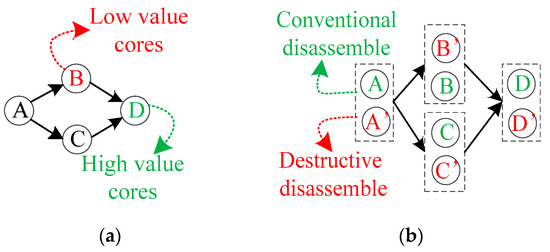
Figure 1.
Different disassembly mode. (a) The conventional disassembly mode; (b). the destructive disassembly mode.
Due to the difference of material, processing technology and other facts, the values of different components vary widely. Such as, the B in red means the part with low value and the D in green means the part with high value. In CDLBP, A, B, C, and D can be disassembled as the normal mode with independently considering the total time, energy consumption, and value of the disassembled parts. In this disassembly mode, it is not economical and environmentally friendly. Such as for the part B, with low value but difficult to disassemble or disassembled with high energy consumption, if it is conventionally disassembled, it will cause greater waste of resources than the value of the obtained part, which is contrary to the original intention of remanufacturing. Conversely, less energy or time may be consumed through destructive disassembly, although the value of obtained parts will be less, the value produced per unit time and energy may be higher. Thus, the disassembly mode and tasks assignment will have a great impact on the efficiency, economy, and environmental protection of the disassembly line.
To address the problem, a novel disassembly mode is proposed, which is shown in Figure 1b. The parts A, B, C, D can be obtained by the normal disassembly mode, or obtain A’, B’, C’, D’ by the destructive disassembly mode. It means that no matter A, B, C, D can be normally removed or not, they always can be destructively disassembled. Obviously, the time, energy consumption, and the value of the obtained parts by the destructive disassembly are certainly different with the conventional disassembly. Therefore, it is no longer appropriate to partially consider the total time or energy consumption in the new disassembly mode. New comprehensive efficiency-oriented optimization metrics are defined, including time efficiency (TE), value efficiency (VE), and energy efficiency (EE). The new disassembly problem is named as multi-efficiency-oriented disassembly line balancing problem (MEoDLBP), and its ultimate goal is to achieve an optimal disassembly sequence (disassemble task assignment) and the disassembly mode (destructive or not) of each part.
2.3. Mathematical Definition and Formulation
Assume that there are parts to be disassembled and each part corresponds to a disassembly task, which can be finished either in normal mode () or in destructive mode (). The task is specified by its processing time , energy consumption , and the value of disassembled part , which depend on the disassembly mode and the use of the disassembled part (reuse, remanufacture, or materials). The tasks need to be finished on workstations in an optimized sequence, and every task must satisfy the disassembly precedence relations. It should be noted that some components cannot be destructively disassembled in the production environment, such as the part with hazardous, high demand, high value, and so forth. Therefore, in order to make the model more generality, if part cannot be destructively disassembled.
Assumptions for MEoDLBP are given as follows:
a. Each task can be finished on any workstation. In fact, hazardous or some special parts may only be disassembled on some fixed workstations. In order to simplify the model, this factor is not considered.
b. The disassembly time, energy consumption, and the value of disassembled part can be obtained through evaluation or historical experience data before disassembly.
c. Since the remanufacture products to be disassembled are classified based on inspection and evaluation, the same batch of remanufacture products can be considered as indistinguishable.
d. The workstations are already setup and the number of workstations is fixed .
e. Destructive disassembly has no effect on the disassembly sequence.
2.3.1. Objective Functions
Time Efficiency
Equation (1) is the calculation of TE. Similar to the traditional disassembly line, the balance of the disassembly line is a direct manifestation of the disassembly efficiency. In order to maximize the utilization of the workstation, TE is defined as the minimum free time of the entire disassembly line, which means that each station’s operating time is as close as the cycle time (CT) [35]. Equation (2) is the calculation of CT, which is the maximum time of M workstations.
Energy Efficiency
Equation (3) is the calculation of EE. It represents the ratio of disassembled parts value to the energy consumed by the disassembly process, which indicates the disassembly value produced by per unit energy consumption. EE considers the contradictory relationship between value and energy consumption, which can overcome the drawbacks of simply pursuing value maximization or minimizing energy consumption in the traditional disassembly mode. The total value of the disassembled parts consists of reuse value, remanufacture value, and material value. The energy consumption includes the energy consumed by each disassembled component through the normal disassembly of energy consumption or destructive disassembly energy consumption.
Value Efficiency
Equation (4) is the calculation of VE. Disassembly time varies wildly due to the difference of assembly process and failure forms. At the same time, owing to the difference of production process and raw materials, the values of remanufactured parts are varying widely. And the components with long disassembly time are not always having high remanufacturing value. Thence, there may be circumstances where it takes long time to disassemble valueless parts in the conventional disassembly mode. Obviously, it is unreasonable. To avoid this phenomenon and maximize both the value and disassembly efficiency of the disassembly line, VE is defined, which is not the maximization of the value obtained from the disassembled parts, but the maximization of the disassembly value in per unit time.
2.3.2. Constrains
Equations (5) and (6) are constrains of the objective functions. Equation (5) represents that any task can be assigned to only one workstation. Constraint 6 indicates that each task must be processed under the given precedence relation set . If task k must be finished before task n, then task k cannot be assigned to the downstream workstation of task n. That is to say, the workstation index of task k should be less than or equal to the workstation index of task n.
3. Multi-Objective Optimization Algorithm for MEoDLBP
The disassembly line balance problem was proved as a kind of NP-complete problem [16,17], which mean that the solving difficulty will increase geometrically with the increase of the problem scale. It is difficult to obtain optimal solutions with traditional mathematical methods, and meta-heuristic method becomes an effective way, such as Ant Colony Algorithm [36], Genetic Algorithm [37,38], Particle Swarm Optimization [12], Tabu Search [39], etc. To validate the solutions generated by algorithms and proving their versatility in accommodating substantial variations in the problem environment, Alshibli utilized Taguchi’s orthogonal arrays to test the robustness of a previously-proposed Simulated Annealing (SA) algorithm [1]. As a new group intelligent optimization algorithm, artificial bee colony algorithm (ABCA) has the characteristics of simple operation, low control parameters, high searching precision, and strong robustness in the optimization of complex problems, and has been widely used for assembly line balancing problem [40,41] as well as DLBP [14]. However, since the classical ABC algorithm is mainly used to solve the continuous problem, the discretization of the solution and generation of new solutions are the focus of research. In this section, a multi-objective optimization method based on non-dominated sorting is proposed after introducing the basic ABC algorithm, which is used to solve the MEoDLBP model.
3.1. Basic Artificial Bee Colony Algorithm
In the ABC algorithm, a food source represents a possible solution of a problem, and the objective value is used to describe its quality. Employed, onlooker, and scout bees are used to search for good food sources. The bee swarm consists of an equal number of employed and onlooker bees, which both are equal to the number of food sources. The steps below describe the operation of the algorithm:
Step 1: Initialization phase. The initial solution can be generated by Equation (7).
where and are the upper and lower bounds for dth variable in the search space, respectively. is the number of food sources, that is the number of the population. is the number of each individual’s variables.
Step 2: Employed bee phase. Employed bees are employed to find a potential solution, which equation can be defined as:
where represents a randomly selected index of bees which is different from that of the current employed bee , . is a randomly generated real value within the interval [−1,1]. After was obtained, it will be compared with , and the better individual will be saved.
Step 3: The onlooker bee phase. The task of onlooker bees is to exploit the region found by employed bees. Each onlooker bee selects a food source based on the following probability :
where denotes the fitness of the i-th food source, is the size of food sources. For any onlooker bee, if a random number within [0,1] is less than the probability of , then the i-th food source is selected. Equation (8) is also adopted in this phase. Onlooker bees apply the same greedy selection strategy to select the better one between the current onlooker bee and the generated .
Step 4: The scout bee phase. If a food source cannot be improved after iterations, it’s associated employed bee becomes a scout bee. The scout bee will generate a new food source according Equation (7), and the old one will be deleted.
3.2. Dual-Population Discrete ABCA
As we all know, the basic ABC algorithm is proposed for solving continuous optimization problems [42], and the solutions of MEoDLBP are discrete. The encoding, decoding, employee bee process must be modified. As a result, the dual-population discrete ABCA (DDABCA) is proposed.
3.2.1. Encoding and Decoding
The decision variables of MEoDLBP are and . is a 0-1 matrix of m rows and n columns. In order to reduce the storage space of the solution and improve the operation efficiency, is encoded as a vector , which contains n elements. The i-th element value x(i) means the i-th process is operated on x(i)-th workstation. is a 0-1 vector containing n elements and d(i) = 1 if the i-th part will be disassembled in destructive mode, otherwise d(I) = 0. Finally, the colony is encoded as a row vector of 2n elements consists of and . The encoding process is shown as Figure 2, in which M = 5, N = 9 and the decoding process are reversed.
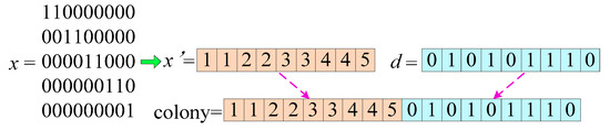
Figure 2.
The process of encoding.
3.2.2. Swap Operations
In this study, a partition swap operation is used in the operation of employee bee process and onlooker bee process. The swap operation is similar with Li [39], but there are big differences due to the difference in encoding, which is designed according to the characteristics of the problem. Since the individual consists of two parts (x and d), so does the swap operation. Firstly, for each employee bee (parent1), randomly selects another individual parent2 (parent2≠parent1). Secondly, randomly choose a swap position in parent1 and randomly choose a swap-able position in parent2 constrained by Equations (5) and (6). Then swap their positions, and four x pieces(x1,x2,x3,x4) and four d pieces(d1,d2,d3,d4) are generated. Based on the pieces, 14 (4 × 4 − 2) new individuals can be obtained through pairwise combinatorial. Compare with parent1 and parent2 and retain the better one to the next generation (Figure 3).
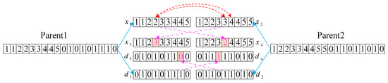
Figure 3.
The swap operation in discrete dual population artificial bee colony algorithm (DDABCA).
3.2.3. Insert Operation
The insert operation is defined to enhance the local search ability of DDABCA. For the problem of MEoDLBP, insert operations are performed independently in the x and d regions. Firstly, randomly select the insertion position and inserted content from the parent. Then put the insertion content in the insertion point and move the content behind the insertion point back. The process of generating child is shown in Figure 4.
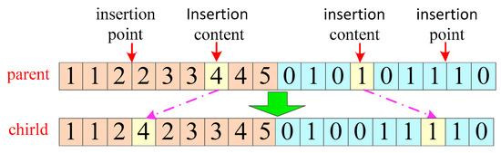
Figure 4.
The insert operation in DDABCA.
3.2.4. Mechanism of Dual-Population
For the multi-objective problem with constraints, the optimal solution may be located on or near the bound boundary, and the fitness value of the infeasible solution near the optimal solution is likely to be better than that of the solution located within the feasible domain. Such infeasible solutions may be more helpful for finding the optimal solution. So, the difficulty of solving such problems is how to effectively make use of the infeasible solutions with good performance during the search process.
In order to preserve some of the infeasible solutions, in this paper, a dual-population search mechanism is proposed, in which stores feasible solutions, stores infeasible solutions, , is the population size, respectively, and . When a new individual is generated, its storage rules are as follows.
Rule1: If is a feasible solution, and the number of feasible solutions in is less than , will be inserted into directly; if the number of feasible solutions in is more than , will be compared with each individual in , if exists in and Pareto dominates , then will be instead by ; if not exists, then insert into , calculate the distance between every two individuals in and randomly delete one of the two closest individuals.
Rule2: If is an infeasible solution, and the number of infeasible solutions in is less than , will be inserted into directly; if the number of infeasible solutions in is more than , will be compared with each individual in , if exists in and Pareto dominates , then will be instead by ; if not exists, then insert into , calculate the distance between every two individuals in , and randomly delete one of the two closest individuals.
Rule3: If is an infeasible solution and it is still infeasible after iterations. Random initializes a feasible solution to instead . This rule is mainly to ensure that infeasible solutions evolve toward feasible solutions, which could improve the conversion rate of the infeasible solution set and improve the efficiency of the algorithm.
The DDABCA is presented as Algorithm 1.
| Algorithm 1. The pseudo code of DDABCA for MEoDLBP |
| 1. Parameter initialization (, , , , , ) |
| 2. Initialize population with all constrains, non-discriminatory sorting and put the top into |
| 3. Iter = 0 |
| 4. Do |
| 5. //Employed bee phase |
| 5.1. for in |
| 5.2. Generate according swap operations for |
| 5.3. if is a feasible solution |
| 5.4. Put into according Rule1 |
| 5.5. else |
| 5.6. Put into according Rule2 |
| 5.7. End if |
| 5.8. End for |
| 5.9. For in |
| 5.10. Generate according swap operations for |
| 5.11. Put into or as 5.3-5.7 |
| 5.12. End for |
| 6. //Onlooker bee phase |
| 6.1. Each onlooker bee selects a source of employed bee using the |
| 6.2. Produces neighborhood solutions according to swap operations and insert operations. Put the neighborhood solutions into or as 5.3-5.7 |
| 7. //Scout bee phase |
| 7.1 Determine the abandoned solution and replace it with a new randomly produced solution |
| 7.2. //Rule3: |
| 7.2.1. For in |
| 7.2.2. If |
| 7.2.3. Randomly produce new solution according swap operations |
| 7.2.4. Put into or as 5.3-5.7 |
| 7.2.5. End if |
| 7.2.6. End for |
| 8. Evaluate fitness of the population and |
| 9. Non-dominated sorting and to obtain the sets of non-inferior front , , and is the Pareto optimal solution set |
| 10. Iter = Iter+1 |
| 11. While (Iter < MaxIter) |
In order to ensure the high efficiency of the algorithm, the maximum number of feasible and infeasible solutions is limited by and , respectively. At the same time, in order to ensure the diversity of the solution, feasible solutions and infeasible solutions are constantly transforming with each other along with the evolution.
4. Validation
The validity and superiority of the proposed method is verified through the disassembly of reducer with 18 tasks [43] and the disassembly of Electronic Tacking Machine (ETM) with 52 tasks [17].
Based on the data in the literatures (disassembly time, disassembly precedence relations, etc.) and the data obtained from surveys and experiments (energy consumption, value of disassembled parts, etc.), MEoDLBP models and CDBLP models are established for the two examples. The Teaching Learning Based Optimization (TLBO), Ant Colony algorithms (AC), and DDABCA are applied to the two problems. The parameters of TLBO and AC are the same as in the literatures [17,43], and the parameters of DDABCA are shown in Table 1. The range means the different parameters have been tested for DDABCA, and the value is the best parameters after the test [44]. All of the algorithms are coded in Matlab programming language and tested on an Intel(R) Core(TM) i5-4430S CPU @ 2.70GHz PC with 4GB RAM. Each algorithm is tested 50 times. In order to make the results comparable, the termination condition for 18 disassembly tasks is the Pareto solution does not change within 5 iterations or the cycle reaches 200 iterations. The termination condition for 52 disassembly tasks is the Pareto solution does not change within 7 rounds or the cycle reaches 500 iterations. The optimization results are shown in Figure 5, in which the abscissa represents different optimization objectives, and the ordinate represents the improvement percentage of MEoDLBP over CDBLP.

Table 1.
The parameters of DDABCA.
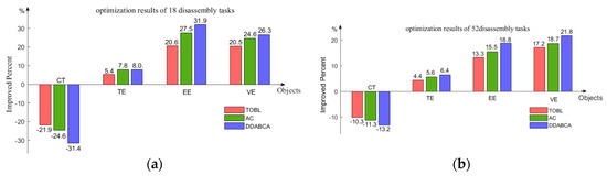
Figure 5.
Optimization results of different algorithms for different tasks scales (a) The optimization results of reducer; (b) the optimization results of Electronic Tacking Machine (ETM).
First of all, from the perspective of different models in Figure 5a, we can see that the cycle time of the MEoDLBP model is greatly reduced compared to the CDBLP model. And the reductions of the algorithms TOBL, AC in the literatures and the DDABCA proposed in this paper are 21.9%, 24.6%, 31.4%, in order. At the same time, the objective functions TE, EE, VE have a great degree of improvement by all algorithms. The maximum degree of improvement for TE, EE, VE reach a staggering 8%, 31.9%, and 26.3% between MEoDLBP and CDBLP. Similar conclusions can also be drawn from Figure 5b. That is to say, for different types of products with different disassembly complexity, the model proposed in this paper is superior to the traditional disassembly model under the indicators of CT, TE, EE, and VE, which means more efficient, energy conservation, and environmentally friendly.
Meanwhile, from the perspective of different algorithms in Figure 5a,b, the optimization result DDABCA proposed in this paper is the best of the three algorithms, the second is AC, and the result of TOBL is the worst. That is to say, algorithm DDABCA has better global optimality.
However, the maximum, average, minimum iteration time of different algorithms for different tasks scales are shown in Figure 6. In Figure 6a, the maximum, average, and minimum iteration time of DDABCA are better than that of AC and TOBL, which means the performance of DDABCA is the best. At the same time, it can be seen from Figure 6a that the iteration time fluctuations range of algorithm DDABCA is the smallest, which means that DDABCA is more robust. This is mainly because the employee bee, observation bee, and scout bee mechanisms of the ABCA ensure its global convergence. At the same time, the dual-population mechanism can better maintain the diversity of population, which enables it to find the optimal solution faster. But when the problem size becomes larger, the dual population mechanism limits its convergence speed, which is shown in Figure 6b. Therefore, how to ensure the efficiency of solving large-scale complex problems will be the direction of our following research.
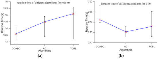
Figure 6.
Iteration time of different algorithms for different tasks scales (a) the iteration time for reducer; (b) the iteration time for ETM.
5. Case study
5.1. Case Description
For the validation of the practicability of the proposed method, the proposed algorithm is applied to solve an automobile engines disassembly line problem based on a field investigation. The structure of the engine is shown as Figure 7, in which only the main parts to be disassembled are included and other parts have been removed.
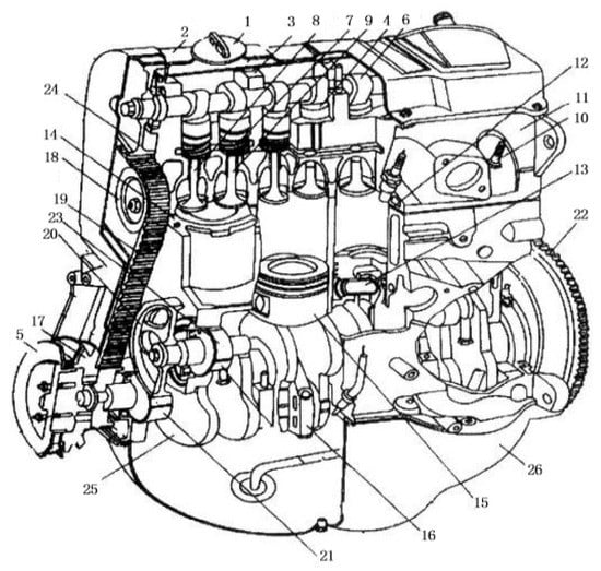
Figure 7.
Automobile engine structure.
In order to determine the remanufacturability of each part, detection and evaluation of the recycled products are usually carried out before disassembly. Then the disassembly time, energy consumption, and value of the disassembled parts in normal disassembly mode or destructive mode could be obtained as Table 2. To improve the accuracy of the data, all the data are based on statistics of remanufacturing historical experience, such as going to Dongfeng Cummins engine remanufacturing factory to collect actual production data, etc. The unit of disassembly time is second. The unit of energy consumption is kWh, and it’s just an equivalence value, which actual may be electricity, mechanical energy, light energy, or chemical energy and so forth. The unit of disassembled parts value is CNY. Crankshaft is the most demanding component for engine remanufacturing, in other words, the Crankshaft cannot be destructively disassembled, which means .
Table 2.
The time, value and energy consumption in different mode.
There are five workstations in the disassembly line. According to the constraints between various components, disassembly priority relationship is shown as Figure 8, and in which also shows the task assignment in CDBLP mode. Such as the task 1, 2, 3, 4, 6, and 7 are finished in the first workstation.
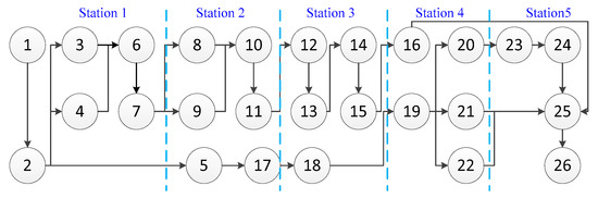
Figure 8.
The disassembly priority relationship in conventional disassembly line balancing problem (CDLBP) model.
5.2. Results
The parameter values of DDABCA are shown as Table 1. Because there are three conflicting objective functions in MEoDLBP model and the improvement of one objective function may lead to deterioration of another, which is known as multi-objective optimization problem. In these kinds of optimizations, no single solution exists that can optimize all objective functions simultaneously. The algorithm to solve the multi-objective optimization problem will find a set of nondominated solutions, which is called Pareto front. It is shown as in Figure 9, and each point * is an optimal solution.
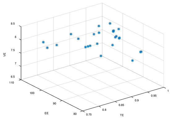
Figure 9.
The Pareto front obtained by DDABCA.
The optimal solution is randomly selected from the Pareto solution set. Based on , the distribution of each process is shown in Figure 10. The distribution of the processes at the five stations is as following: {1, 2, 3, 4, 5, 17}, {18, 19, 21, 22}, {6, 7, 8, 9, 20, 23}, {10, 11, 12, 13, 14, 15, 16}, {24, 25, 26}. The process in dotted circle means it is disassembled in destructive mode and the others are disassembled in conventional mode. Such as part 1, 2, 3 et al. are disassembled in destructive mode and part 4, 6, 7 et al. are disassembled in normal mode.
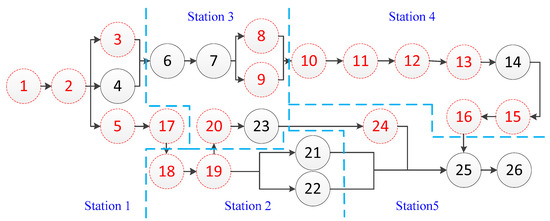
Figure 10.
The disassembly priority relationship in multi-efficiency- oriented disassembly line balancing problem (MEoDLBP) mode.
The time, energy, values of the solution are listed in Table 3, which are compared with the optimal solution in CDLBP mode. It shows that although the value of disassembled parts in CDLBP mode is higher than that in MEoDLBP mode, the final result is contrary as Table 4 shows. In destructive disassembly mode, the CT is reduced about 47.40%, the TE, EE, and VE are improved about 9.65%, 52.01%, and 25.92%, respectively, which indicate higher disassembly efficiency, higher profits in per unit of energy consumption, and higher profits in per unit of time. The reason for this lies in some valueless parts, such as part 1, part 2, part 9, etc., are disassembled with high time and energy consumption in CDLBP mode, but lower time and energy consumption in MEoDLBP mode. Eventually the time and energy consumption in MEoDLBP mode is much less than that in CDLBP mode.
Table 3.
The time, energy, value of MEoDLBP and CDLBP in each station.
Table 4.
The optimal solution of MEoDLBP and CDLBP.
6. Conclusions
In this paper, a novel multi-efficiency-oriented disassembly line balance model is presented, and the objective functions of time efficiency, value efficiency, energy efficiency are defined. For the multi-efficiency-oriented disassembly line balancing problem, a discrete dual population artificial bee colony algorithm is proposed, and two examples are used to validate the proposed model and algorithm. Finally, the methodology was applied to an engine disassembly line. Compared to CDLBP, the results show that the CT is reduced about 47.40%, the TE is improved about 9.65%, the EE is improved about 52.01%, and the VE is improved about 25.92%.
The methodology proposed in this paper provides decision makers with more economical and sustainable decisions. Existing studies consider more disassembly time, cost, and demand, while ignoring the value of parts and energy consumption of disassembly. Although the cost of disassembly may be lower and the disassembly time may be shorter, the natural resources consumed to generate unit value may be more. Obviously, it is a non-sustainable disassembly method. The MEoDLBP proposed in this paper just makes up for this shortcoming. At the same time, decision makers can choose the optimal solution from multi-objective optimization solutions according to their preferences.
However, there are still some limitations in our research. Firstly, the disassemble time, value, and energy consumption of the product were only obtained through statistics or historical experience. It is too complicated, and some efficient and accurate data acquisition method requires further study. Secondly, the method has been verified by only three instances. More experiments need to be conducted, and more instance data needs to be obtained on different products, such as printer, metallurgical equipment, etc.
Author Contributions
All authors contributed to design of the study protocol and helped with drafting the manuscript. The following specific contributions apply: J.C. and X.X. developed the research concept and methodology. J.C. undertook data analysis and interpretation. L.W. developed data collection tools and supervised data collection. Z.Z. supervised data management. J.C. and X.L. developed the intervention content. All authors contributed to the manuscript.
Funding
This work was supported by the National Natural Science Foundation of China (No. 51805385, 51604196, 71471143); Natural Science Foundation of Hubei Province (No.2018CFB265); Student Science and Technology Innovation Fund of Wuhan University of Science and Technology [No. 17ZRA038].
Acknowledgments
Thanks for all the authors of the references who gives us inspirations and helps. The authors are grateful to the editors and anonymous reviewers for their valuables comments that improved the quality of this paper.
Conflicts of Interest
The authors declare no conflict of interest.
References
- Alshibli, M.; ElSayed, A.; Kongar, E.; Sobh, T.; Gupta, S. A Robust Robotic Disassembly Sequence Design Using Orthogonal Arrays and Task Allocation. Robotics 2019, 8, 20. [Google Scholar] [CrossRef]
- Vinodh, S.; Nachiappan, N.; Kumar, R.P. Sustainability through disassembly modeling, planning, and leveling: A case study. Clean Technol. Environ. Policy 2012, 14, 55–67. [Google Scholar] [CrossRef]
- Güngör, A.; Gupta, S.M. Disassembly line in product recovery. Int. J. Prod. Res. 2002, 40, 2569–2589. [Google Scholar] [CrossRef]
- Mcgovern, S.M.; Gupta, S.M. A balancing method and genetic algorithm for disassembly line balancing. Eur. J. Oper. Res. 2007, 179, 692–708. [Google Scholar] [CrossRef]
- Ding, L.; Feng, Y.; Tan, J. A new multi-objective ant colony algorithm for solving the disassembly line balancing problem. Int. J. Adv. Manuf. Technol. 2010, 48, 761–771. [Google Scholar] [CrossRef]
- Özceylan, E.; Kalayci, C.B.; Güngör, A.; Gupta, S.M. Disassembly line balancing problem: A review of the state of the art and future directions. Int. J. Prod. Res. 2019, 57, 4805–4827. [Google Scholar] [CrossRef]
- Deniz, D.; Ozcelik, F. An extended review on disassembly line balancing with bibliometric social network and future study realization analysis. J. Clean. Prod. 2019, 225, 697–715. [Google Scholar] [CrossRef]
- Smith, S.; Hsu, L. Partial disassembly sequence planning based on cost-benefit analysis. J. Clean. Prod. 2016, 139, 729–739. [Google Scholar] [CrossRef]
- Koc, A.; Sabuncuoglu, I.; Erel, E. Two exact formulations for disassembly line balancing problems with task precedence diagram construction using an AND/OR graph. IIE Trans. 2009, 41, 866–881. [Google Scholar] [CrossRef]
- Tuncel, E.; Zeid, A.; Kamarthi, S. Solving large scale disassembly line balancing problem with uncertainty using reinforcement learning. J. Intell. Manuf. 2014, 25, 647–659. [Google Scholar] [CrossRef]
- Özceylan, F.; Paksoy, T.; Bektaş, T. Modeling and optimizing the integrated problem of closed-loop supply chain network design and disassembly line balancing. Transport Res. E-Log. 2014, 61, 142–164. [Google Scholar] [CrossRef]
- Kalayci, C.B.; Gupta, S.M. A particle swarm optimization algorithm with neighborhood-based mutation for sequence-dependent disassembly line balancing problem. Int. J. Adv. Manuf. Technol. 2013, 69, 197–209. [Google Scholar] [CrossRef]
- Mcgovern, S.M.; Gupta, S.M. Ant colony optimization for disassembly sequencing with multiple objectives. Int. J. Adv. Manuf. Technol. 2006, 30, 481–496. [Google Scholar] [CrossRef]
- Kalayci, C.B.; Gupta, S.M. Artificial Bee Colony Algorithm for Solving Sequence-Dependent Disassembly Line Balancing Problem. Expert. Syst. Appl. 2013, 40, 7231–7241. [Google Scholar] [CrossRef]
- Kalayci, C.B.; Hancilar, A.; Gungor, A.; Gupta, S.M. Multi-objective fuzzy disassembly line balancing using a hybrid discrete artificial bee colony algorithm. J. Manuf. Syst. 2015, 37, 672–682. [Google Scholar] [CrossRef]
- Mcgovern, S.M.; Gupta, S.M. Combinatorial optimization analysis of the unary NP-complete disassembly line balancing problem. Int. J. Prod. Res. 2007, 45, 4485–4511. [Google Scholar] [CrossRef]
- Ding, L.P.; Tan, J.R.; Feng, Y.X.; Gao, Y.C. Multi-objective optimization for disassembly line balancingbased on Pareto ant colony algorithm. Comput. Integr. Manuf. Syst. 2009, 15, 1406–1413. [Google Scholar] [CrossRef]
- Wang, K.; Zhang, Z.; Mao, L. A Pareto Artificial Fish Swarm Algorithm for Multi-objective Disassembly Line Balancing Problems. Zhongguo Jixie Gongcheng 2017, 28, 183–190. [Google Scholar] [CrossRef]
- Zhu, L.; Zhang, Z.; Wang, Y. A Pareto firefly algorithm for multi-objective disassembly line balancing problems with hazard evaluation. Int. J. Prod. Res. 2018, 56, 7354–7374. [Google Scholar] [CrossRef]
- Jia, L.; Shuwei, W. A proposed multi-objective optimization model for sequence-dependent disassembly line balancing problem. In Proceedings of the 2017 3rd International Conference on Information Management (ICIM), Chengdu, China, 21–23 April 2017. [Google Scholar] [CrossRef]
- Ilgin, M.A.; Akçay, H.; Araz, C. Disassembly line balancing using linear physical programming. Int. J. Prod. Res. 2017, 55, 1–12. [Google Scholar] [CrossRef]
- Paksoy, T.; Güngör, A.; Özceylan, E.; Hancilar, A. Mixed model disassembly line balancing problem with fuzzy goals. Int. J. Prod. Res. 2013, 51, 6082–6096. [Google Scholar] [CrossRef]
- Seidi, M.; Saghari, S. The Balancing of Disassembly Line of Automobile Engine Using Genetic Algorithm (GA) in Fuzzy Environment. Ind. Eng. Manag. Syst. 2016, 15, 364–373. [Google Scholar] [CrossRef]
- Wen, H.; Liu, M.; Liu, C. Scheduling method for recycled engine disassembly under uncertainty. Comput. Integr. Manuf. Syst. 2015, 21, 1279–1286. [Google Scholar] [CrossRef]
- Altekin, F.T.; Akkan, C. Task-failure-driven rebalancing of disassembly lines. Int. J. Prod. Res. 2012, 50, 4955–4976. [Google Scholar] [CrossRef]
- Avikal, S.; Mishra, P.K.; Jain, R. A Fuzzy AHP and PROMETHEE method-based heuristic for disassembly line balancing problems. Int. J. Prod. Res. 2014, 52, 1306–1317. [Google Scholar] [CrossRef]
- Dong, J.; Gibson, P.; Arndt, G. Disassembly sequence generation in recycling based on parts accessibility and end-of-life strategy. Proc. Inst. Mech. Eng. Part B 2007, 221, 1079–1085. [Google Scholar] [CrossRef]
- Rickli, J.L.; Camelio, J.A. Partial disassembly sequencing considering acquired e nd-of-life product age distributions. Int. J. Prod. Res. 2014, 52, 7496–7512. [Google Scholar] [CrossRef]
- Kuo, T.C. Waste electronics and electrical equipment disassembly and recycling using Petri net analysis: Considering the economic value and environmental impacts. Comput. Ind. Eng. 2013, 65, 54–64. [Google Scholar] [CrossRef]
- Song, X.; Pan, X. Electromechanical product disassembly sequence planning based on partial destruction mode. Comput. Integr. Manuf. Syst. 2012, 18, 927–931. [Google Scholar] [CrossRef]
- Chen, X.; Lou, P. Product disassembly sequence planning based on partial destruction mode. Nanjing Hangkong Hangtian Daxue Xuebao 2014, 46, 945–950. [Google Scholar] [CrossRef]
- Altekin, F.T.; Kandiller, L.; Ozdemirel, N.E. Profit-oriented disassembly-line balancing. Int. J. Prod. Res. 2008, 46, 2675–2693. [Google Scholar] [CrossRef]
- Ren, Y.; Yu, D.; Zhang, C.; Tian, G.; Meng, L.; Zhou, X. An improved gravitational search algorithm for profit-oriented partial disassembly line balancing problem. Int. J. Prod. Res. 2017, 55, 7302–7316. [Google Scholar] [CrossRef]
- Hezer, S.; Kara, Y. A network-based shortest route model for parallel disassembly line balancing problem. Int. J. Prod. Res. 2015, 53, 1849–1865. [Google Scholar] [CrossRef]
- Hu, Y.; Zhang, Z.; Li, M. Improved bacteria foraging optimization for disassembly line balancing problem. Comput. Eng. Appl. 2016, 52, 258–262. [Google Scholar] [CrossRef]
- Tiwari, M.K. A collaborative ant colony algorithm to stochastic mixed-model U-shaped disassembly line balancing and sequencing problem. Int. J. Prod. Res. 2008, 46, 1405–1429. [Google Scholar] [CrossRef]
- Xia, X.; Liu, W.; Zhang, Z.; Wang, L.; Cao, J.; Liu, X. A Balancing Method of Mixed-model Disassembly Line in Random Working Environment. Sustainability 2019, 11, 2304–2319. [Google Scholar] [CrossRef]
- Kalayci, E.G.; Azizoğlu, M.; Yeralan, S. A disassembly line balancing problem with fixed number of workstations. Eur. J. Oper. Resh. 2016, 249, 592–604. [Google Scholar] [CrossRef]
- Alshibli, M.; Sayed, A.E.; Kongar, E.; Sobh, T.M.; Gupta, S.M. Disassembly Sequencing Using Tabu Search. J. Intell. Robot. Syst. 2016, 82, 69–79. [Google Scholar] [CrossRef]
- Jia, L.; Shuwei, W. Balancing Disassembly Line in Product Recovery to Promote the Coordinated Development of Economy and Environment. Sustainability 2017, 9, 309. [Google Scholar] [CrossRef]
- Li, X.; Peng, Z.; Du, B.; Guo, J.; Xu, W. Hybrid artificial bee colony algorithm with a rescheduling strategy for solving flexible job shop scheduling problems. Comput. Ind. Eng. 2017, 113, 10–26. [Google Scholar] [CrossRef]
- Kiran, M.S. The continuous artificial bee colony algorithm for binary optimization. Appl. Soft Comput. 2015, 33, 15–23. [Google Scholar] [CrossRef]
- Xia, X.; Zhou, M.; Wang, L.; Cao, J. Remanufacturing Disassembly Service Line and the Balancing Optimization Method. Comput. Integr. Manuf. Syst. 2018, 24, 120–129. [Google Scholar]
- Nilakantan, J.M.; Li, Z.; Tang, Q.; Nielsen, P. Multi-objective co-operative co-evolutionary algorithm for minimizing carbon footprint and maximizing line efficiency in robotic assembly line systems. J. Clean. Prod. 2017, 156, 124–136. [Google Scholar] [CrossRef]


© 2019 by the authors. Licensee MDPI, Basel, Switzerland. This article is an open access article distributed under the terms and conditions of the Creative Commons Attribution (CC BY) license (http://creativecommons.org/licenses/by/4.0/).