Article

Soil Properties Spatial Variability and Delineation of Site-Specific Management Zones Based on Soil Fertility Using Fuzzy Clustering in a Hilly Field in Jianyang, Sichuan, China

1
Soil Ecology Lab, College of Resources and Environmental Sciences, Nanjing Agricultural University, Nanjing 210095, China
2
Soil Science Department, Faculty of Agriculture, Zagazig University, Zagazig 44511, Egypt
3
State Key Laboratory of Soil and Sustainable Agriculture, Institute of Soil Science, Chinese Academy of Sciences (CAS), Nanjing 210008, China
*
Author to whom correspondence should be addressed.
Sustainability 2019, 11(24), 7084; https://doi.org/10.3390/su11247084
Submission received: 17 October 2019 / Revised: 3 December 2019 / Accepted: 5 December 2019 / Published: 11 December 2019
(This article belongs to the Section Sustainable Agriculture)

Abstract

:
Avoiding soil degradation and improving crop productivity could be achieved by performing sustainable soil nutrient management with an appropriate understanding of soil properties’ spatial variability. The present fertilizer recommendations for the region where the study area is located are typically symmetric for large regions. This leads to the under-application of fertilizers in zones with low nutrient contents and over-application in zones with high nutrient contents. Therefore, this study was conducted to assess soil management zones (MZs) in the study area for effective soil nutrient management and to evaluate soil properties’ spatial variability. A total of 100 geo-referenced soil samples were collected at a depth of 0–20 cm, processed and analyzed for pH, available nitrogen (AN), available phosphorus (AP), available potassium (AK), soil organic carbon (SOC), total nitrogen (TN) and total phosphorous (TP), while C:N, C:P and N:P ratios were calculated. Soil properties’ coefficients of variation (CVs) widely varied from low (1.132%) to moderate (45.748%). Ordinary kriging and semi-variogram analysis showed differed spatial variability patterns for the studied soil properties with spatial dependence ranged from weak to strong. MZs were delineated by performing principal component analysis (PCA) and fuzzy K-means clustering. Four PCs with eigen values more than 1 dominated 84.44% of the total variance, so they were retained for clustering analysis. Three MZs were delineated based on the two criteria modified partition entropy (MPE) and fuzzy performance index (FPI). The studied soil properties differed significantly among MZs. Thus, the methodology used for MZ delineation could be used effectively for soil site-specific nutrient management for avoiding soil degradation concurrently with maximizing crop production in the study area.

1. Introduction

Soil degradation due to inadequate agriculture practices has become a global problem [1], which is clearly appearing in China due to fertilization mismanagement and the over exploitation of agricultural lands. China’s population has increased rapidly during the last 50 years, likewise the production of the main crops has increased. However, such increases in productivity have been mainly attained by using unsustainable agricultural practices and inadequate and imbalanced fertilization. On the other hand, a depletion in soil nutrients occurs due to increasing crop yield in the land unit area, which will cause detrimental impacts on agricultural productivity in the future [2]. Whereas, the topsoil degradation due to soil erosion, decreased soil organic matter and soil nutrients content which led to decreasing soil fertility and consequently declining crop production [3,4,5,6,7]. One of the most roughly eroded regions in the Upper Yangtze River Basin is Sichuan Basin which is dominated by hilly areas [8], where the study area is located. Therefore, intensifying agriculture using balanced fertilization and environmentally sustainable practices will be the best solution for China.
Soil has a heterogeneous structure and its status affects ecosystem processes which control nutrients cycling [9]. Avoiding soil degradation and improving soil health and fertility level could be achieved by performing sustainable soil management with an appropriate understanding of soil properties [10,11]. Soil properties spatial variability is affected by farming management practices, such as irrigation and fertilization, as well as soil formation factors, like soil parent materials [12]. Therefore, managing field areas as a uniform unit oftentimes causes the treating of high nutrient content areas with over application of inputs, and treating low nutrient content areas with insufficient input applications [13,14], which leads to soil degradation. The effects of soil nutrients spatial variation on crop yields is clearly observed in cultivated sloping lands. However, what is known about soil nutrients spatial variation mechanism is still little [8,15]. If the spatial variation mechanism of soil nutrients is better understood, it will be possible to control its negative effects on agriculture production by using suitable soil management practices [8].
Precision agriculture is an idea for handling natural resources and understanding sustainable agricultural development [16]. Soil variation must be characterized quantitatively and locally to achieve the objectives of precision agriculture, in which the perfect benefits of environmental protection and profitability could be attained by matching each of the agricultural practices and land use with the local conditions [17,18,19]. Precision Agriculture was founded on the evaluation of within-field variation; hence the delineation of management zones is crucial for facilitating variable managing among the different zones [20]. The evaluation of soil properties spatial distribution could be conducted by using geostatistical methods [21]. Values of different soil properties at un-sampled locations could be predicted using geostatistical estimation by accounting the spatial correlation between sampled and estimated points, which results in reducing involved costs and estimation error [22]. Hence, geostatistics is essential for sustainable agriculture, as it provides valuable information about soil properties; this information contributes to knowing what, when, where, and how much farming inputs will maintain soil productivity and minimize costs concurrently with decreasing the environmental impact [23]. So, an appropriate understanding of soil properties spatial distribution could be used for soil site-specific management for sustaining crop and soil productivity by variable rate addition of nutrients [24,25,26,27].
Understanding the relationship between soil characteristics and spatially varied fertility was urgently needed due to the public concern about maximizing soil productivity and crop inputs efficiency [28,29]. Therefore, it was necessary to delineate site-specific management zones [30]. The most general approach used to manage within-field spatial variability was management zones (MZs) [31] because MZs are symmetric sub-regions with similar characteristics affecting yield or with the same yield productivity [32]. Also, they could be defined as sub-areas with equal potential productivity. A soil sampling grid was optimized by Khosla and Alley [33] by using homogenous management zones. Also, nutrient maps for fertilizer application with variable rates were developed based on management zones by Fleming et al. [34]. Soil properties’ spatial variability might also be delineated by locating within field spatially coherent areas [35].
Principal component analysis (PCA) and fuzzy means classification were frequently used to delineate soil MZs in different agriculture ecosystems with different crops [26,36,37]. A related set of data could be summarized into a few expressive components by performing principal component analysis (PCA) [38]. Kriging methods could be used in mapping principal component values [39]. MZs could be delineated by using the principal components (PCs) scores to perform the clustering analysis [40].
Soil chemical properties were influenced by soil organic carbon (SOC) and soil pH among soil traits, as they affect the soil nutrients’ availability [41]. Soil nutrients availability was affected by soil pH, while chemical reactions and the physical and biological environment in the soil were modified by SOC [37]. The ecosystem production capacity was directly affected by SOC [42]. Also, total nitrogen (TN) and total phosphorus (TP) were considered to be from the most important indicators of soil productivity and fertility [43]. For plant growth soil N and P were major nutrient elements, which influence the photosynthesis process and other processes related to plant production [44]. Moreover, soil N and P cycles were associated with the SOC cycle [45], and had the ability to alleviate global climate change effects [46,47,48]. Hence, for the sustainable development of soil OC, N, P and their stoichiometry variations must be better understood to assess the status of nutrients in soil ecosystems. Furthermore, soil C:N ratio is considered to be a useful indicator of soil organic matter decomposition [49,50], whereas, by adding fertilizers soil N:P ratio was changed, thus it has a potential diagnostic value [51]. Besides, according to Tian et al. [52], soil phosphorous suppling capacity depended on the soil content of TN and the parent material weathering stage, which was varied by spatial heterogeneities.
However, information concerning soil properties’ spatial variability and soil MZs in the Jianyang–Sichuan province is still limited, which leads to the uniform management of Sichuan soils, which may result in soil degradation due to the over and under application of agricultural inputs. Thus, the present study was carried out to (1) evaluate soil properties’ spatial distribution using geostatistics, in addition to (2) classifying the study area into MZs based on the status of soil nutrients using PCA and fuzzy K-mean cluster analysis.

2. Materials and Methods
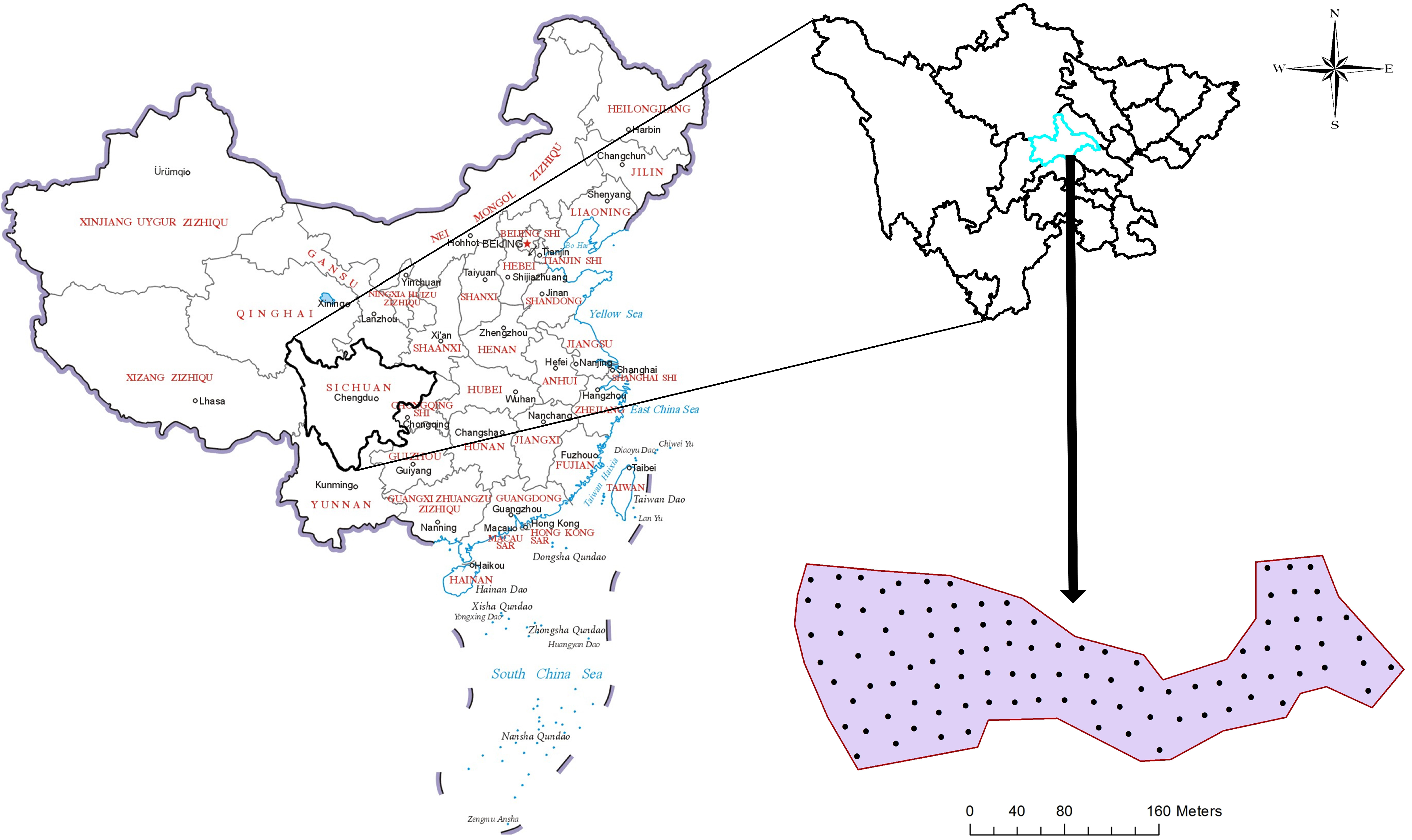
2.1. The Study Area

The study was carried out in a field of 9.22 ha in Jianyang, Sichuan basin, Sichuan Province, China, situated at (30° 30′ 49.85” N and 104° 38′ 14.91” E) (Figure 1). The area’s climate was described as subtropical humid, receiving an average annual rainfall of 944 mm. Summers had a good deal of rainfall, while the winters had very little. The mean highest temperature (33 °C) was recorded in July while the mean lowest temperature (11 °C) was recorded in January. The mean highest relative humidity (77%) was obtained in September and the mean lowest relative humidity (47%) was obtained in December. The soil of the study area weathered from purple sandstone and mudstone, and according to the soil classification of FAO (Food and Agriculture Organization) it was classified as Regosols. Four texture classes were found in the study area including clay loam, silty clay loam, silt loam and loam. The study area was planted with corn at the sampling time.

2.2. Collection and Analysis of Soil Samples

A total of 100 soil samples were collected at a depth of (0 to 20 cm) based on an almost regular grid of 30 × 30m within the study area. Three soil subsamples were gathered using hand auger from a radius of one meter from each sampling location. These subsamples were mixed to get a representative soil sample for each sampling location. Sampling locations were obtained by using a Global Positioning System (GPS) hand-held device, in which latitude and longitude geographical coordinates were recorded for each sampling point. The obtained soil samples were air-dried, while debris and stones were discarded. By using a wooden pestle, the soil samples were grinded, then each soil sample was passed out of a 2 mm sieve and then were stored in polyethylene bottles to estimate each of soil pH, AN, AK and AP. A part of the 2 mm screened samples were re-sieved through a 0.15 mm sieve and saved in polyethylene bottles to determine each of SOC, TN and TP.
Soil pH was estimated in a soil water suspension of 1:2.5 (w/v) [53]. The content of SOC was evaluated by the method of Walkley and Black [54]. TN was estimated by the Kjeldahl method [55]. By using a spectrophotometer, TP was estimated [56]. AN was evaluated using the Micro -Kjeldhal procedure [57] and AP was tested following the way of Olsen [58], while AK was delineated using Flame photometer [59]. C:N, C:P and N:P ratios were calculated by dividing SOC by TN, SOC by TP and TN by TP, respectively. The international pipette method [60] was used to delineate the soil texture in only 50 samples representing the study area.

2.3. Descriptive Statistics

Descriptive statistics, like mean, minimum, maximum, coefficient of variation (CV) and stander deviation (SD), of the studied soil properties were delineated by using IBM SPSS 23 statistics software, Armonk, New York, U.S.A. Skewness and kurtosis were calculated for the studied soil properties to perform the test of normality for each of them. Except for AP, all the other soil properties passed the test. So, before analyzing the data geostatistically, AP scores were transformed, performing the natural logarithm to be distributed normally. Then, using a weighted back transformation technique, the data were back transformed. The relationships between the ten soil properties were evaluated by obtaining the values of Pearson’s correlation coefficient.

2.4. Geostatistical Analysis

For evaluating the spatial variation pattern of the studied soil properties, a semi-variogram was calculated for each soil property using Equation (1) by utilizing ArcGIS 10.4.1 software.
γ ( h ) = 1 2 N ( h ) α = 1 N ( h ) [ z ( X a + h ) ] 2 00
where: γ(h) represents the semivariance for the lag distance (h), N (h) is the samples pairs number which separated by (h), z(xα) is the sample’s measured value at the sampling location (αth) and z(xα + h) is the sample’s measured value at the location (h + αth). Semi-variogram models like stable, circular, Gaussian, exponential and spherical, were estimated to delineate the best fitted model for each soil property.
The cross-validation technique was performed to choose the best fitted semi-variogram model for each of the studied soil properties, that is, by comparing the estimated values which were kriged by using the semi-variogram model with the actual values. So, mean error (ME) was calculated for each model to delineate the best fitted one for each soil property, in which the best is the model with the lowest (ME) value, as it has the highest prediction accuracy.
M E = i = 1 n [ z ( x i ,   Y i   ) z × ( x i ,   Y i   ) ] n
In which n is each case number of observations, z(xi, yi) is the observed soil property, z × (xi, yi) is the estimated soil property, and (xi, yi) is the soil sample coordinates.
The values of the different soil properties were estimated at the un-sampled locations for each property using the ordinary kriging (OK) method [61]. The OK technique was performed because it is the most reliable of all predicting techniques based on (ME) [62]. OK is also the best unbiased predicting method in cases in which the soil samples locations were selected randomly and sparse to predict the values of the soil properties at the un-sampled point. It also reduces the outliers’ impact as one of its most important benefits [63].

2.5. Principal Component Analysis

To summarize the principal sources of the data variation between the correlated variables, principal component analysis (PCA) was used, as it is a multivariate analysis method for dimension reduction which uses the correlated variables to recombine and identify the orthogonal linear of the variables. Instead of a covariance matrix a correlation matrix including the studied soil properties was inputted for the PCA, so that a normalized PCA resulted. The number of the principal components (PCs) must be equal to the number of the variables inserted to the analysis. Only PCs with high eigen values were considered to be the best to represent the studied properties [64]. In this study the management zones were delineated by using the scores of PCs with eigen values more than 1 in the clustering analysis.

2.6. Fuzzy k-Means Clustering Algorithm

The commonly used fuzzy k-means classification method was performed to divide the datasets into diverse clusters; each one has its common characteristics [30]. By using FuzMe software, the study area was parted into two to seven clusters (with settings of maximum zones = 7, minimum zones = 2, maximum iteration = 300, fuzziness exponent = 1.5 and stopping criterion = 0.0001) [65]. For a practical use of the MZs, the maximum number of clusters was considered to be seven.
To delineate the optimal number of classes, the two quantitative estimation criteria modified partition entropy (MPE) [66] and fuzziness performance index (FPI) [67] were used, and they could be calculated by using the following equations:
F P I = 1 N N 1 [ 1 i = 1 N j = 1 K   ( µ i . j m ) 2 / k ]
M P E = 1 N l o g k i = 1 N j = 1 k µ i . j m l o g ( µ i . j m ) .
In which N is the number of soil samples; k is the number of classes; m is the weighting exponent of fuzziness; μij is the fuzzy membership and log is the natural logarithm. MPE estimates the amount of defective created by precise classes and FPI measures the fuzziness degree. The MPE depicts the uncertainty (or certainty) of fuzzy k-classification in which MPE = 1 refers to the maximum uncertainty and MPE = 0 means the maximum certainty. The FPI defines the membership sharing between each couple of fuzzy clusters, in which FPI = 1 refers to the maximum fuzziness and FPI = 0 means non-fuzziness. The optimum number of clusters was obtained against the minimum values of MPE and FPI. By using t-test analysis, the variance of each studied soil property across the management zones were evaluated.

3. Results and Discussion

3.1. Variability of Soil Properties

The studied soil properties’ descriptive statistics are given in (Table 1). The soil of the study area tended to be a somewhat alkaline, with a pH ranging between 7.85 and 8.31. The mean SOC and TN were 9.58 and 0.98 g/kg, respectively. According to the soil nutrient classification standard in China [68], the means of SOC and TN content were low in the study area, while the mean soil AK and AP content were medium with a value of 147.10 and 17.02 mg/kg, respectively. Whereas the mean AN content was 35.42 mg/kg, which indicated that the study area’s AN content was very low. This shortfall in SOC, TN and AN might be due to removing the topsoil which is caused by water erosion, resulting in reducing soil nutrients and organic matter [6].
The soil C:N, C:P, and N:P ratios were considered to be good indicators of the soil nutrients status during soil development [52]. The high C:N ratio (>25) indicated that soil organic matter accumulation was faster than its decomposition [69]. As shown in Table 1, soil C:N ratio ranged between 4.28 and 14.83 with a mean value of 9.83, indicating a complete breakdown of soil organic matter in the study area. Bui and Henderson [50] reported similar results. Also, our results showed that soil C:P ratio values ranged from 4.46 to 20.48, when the mean value was 11.65, implying a phosphorous net mineralization. In which Paul [49] recorded that C:P ratio <200 referred to a net mineralization, while C:P ratio >300 referred to a net immobilization, and a C:P ratio ranging from 200 to 300 implied little change in the concentrations of soil soluble P. Our results revealed that the N:P ratio ranged between 0.77 and 1.68, with a mean value of 1.19, which indicated high microbial activity, whereas due to Wang et al. [70] the N:P ratio was negatively correlated with microorganisms’ activity and biomass in which N:P > 2 indicated biomass decline.
All soil properties were normally distributed with non-significant skewness except AP, which skewed with a value of 1.13. The lowest CV (1.13%) was for soil pH, while the highest CV (45.75%) was for AP, which was in line with Wang et al. [71]. Also, Karaman et al. [72] reported that AP was usually more variable than most of the other soil properties. According to Jakobsen [73], the CV of the different soil properties ranged from low (<10%) to moderate (10 to 100%). High CVs for the remaining soil properties revealed considerable spatial variability and so it was suggested to use nutrient site-specific management to improve the study area soil productivity.

3.2. Correlations Between Soil Properties

The degree of correlation among the ten soil properties is shown in Table 2. Most of the soil properties were significantly positively and negatively correlated with each other, showing similar and opposite spatial distribution patterns, respectively. AN, AP, AK, TN and TP were negatively correlated with soil pH, indicating that increasing N, P and K availability could be significantly achieved by decreasing soil pH in the zones with low concentrations of these nutrients. Soil AN and AP were positively correlated with SOC, in which SOC was an important portion of the soil which affected soil chemical, physical and biological properties influencing soil nutrients’ availability [37].
The concentrations of SOC, TN and TP had a significant positive correlation withbetween each other, and the comparatively high correlation coefficients (0.572) for soil SOC and TN and (0.562) for TN and TP, indicated that the C:N and N:P ratios were highly constrained. Also, a comparatively constrained C:P ratio was founded on the correlation coefficients of 0.274 for the SOC and TP concentrations. Ouyang et al. [74] obtained the same results for C:N and C:P ratios, and a different result for N:P ratio. Correlations among these properties revealed that PCA should be used to summarize the principal sources of data variance.

3.3. Soil Properties Spatial Distribution

As shown in Table 1, distributions of all the studied variables were lightly skewed (skewness ˂ 1), and their means were close to their medians, except soil AN which skewed with a value of 1.13, so that before performing geostatistical analysis its values were log-transformed. Table 3 and Figure 2 show the parameters of the studied soil properties semi-variogram. Soil TN, pH, AP, AK, C:N, C:P and N:P were best modeled by using spherical models. Also, several authors found that most of the soil properties were best modeled by using spherical models [75,76,77] while TC, TP and AN were fitted best with stable models.
Cambardella et al. [78] reported that nugget to sill ratio value <0.25 reveals strong spatial dependence due to the intrinsic (inherent) factors like soil texture and mineralogy, while when the ratio’s value was between 0.25 and 0.75, it referred to moderate spatial dependence due to the extrinsic and intrinsic factors, whereas a ratio’s value >0.75 referred to weak spatial dependence due to the extrinsic factors like fertilization and tillage. The soil properties of this study had diverse spatial dependence due to their nugget to sill ratios. Soil AN had strong spatial dependence, whereas SOC, TN, AP, AK, C:N ratio and C:P ratio had moderate spatial dependence. Soil pH, TP and N:P ratio had weak spatial dependence, as shown in Figure 2, which might be due to the weak spatial distribution of these properties and hence it was recommended to carry out extra research based on a large scale sampling design to capture the spatial distribution of these variables.
The maximum distance in which spatial dependence or autocorrelation exists was defined as the range value of semi-variogram. As shown in Table 3, the range values of soil properties in this study ranged between 48 m for AK and 679 m for SOC. Larger than the obtained range values, spatial dependence does not exist for these soil properties. Lopez-Granados et al. [75] reported that a large range value indicated that estimated soil properties were influenced by anthropogenic and natural factors over larger distances than the other soil properties which have smaller ranges.
The distance between soil samples should be below half the semi-variogram range value [79]. Hence, the obtained range values for soil properties in this study could be used for planning the future soil sampling in the study area for geostatistical research by taking samples at interval distances less than half the obtained range values of the studied soil properties.
Cross-validation technique was performed to get the most precise predictions with the lowest ME values for the studied soil properties as shown in Table 3. According to Shaddad et al. [80], the lowest ME values revealed that soil properties kriging predictions were closer to the estimated values, while the MSSE value for each of the studied soil properties should be one; however, if the MSSE value was different from one but still within the tolerance interval 1 ± 3 (2/N)1/2, in which N was the number of soil samples, the model was considered to be accurate. The tolerance interval had ranged from 0.576 to 1.424 and as shown in Table 3. MSSE values for all soil properties were within this range, which referred to the high prediction accuracy of the semi-variograms models used for all the soil properties.
Figure 3 showed the distribution maps of the studied soil properties. The eastern part of the study area had the lowest content of soil TN, which had a similar distribution pattern to soil AN, due to the presence of a strong positive correlation between soil TN and AN. Soil AK was low in most of the study area parts. Soil AP was low in the west part of the study area. It can be clearly noticed that high pH distributed in the east and small regions in the center and the west of the area. As shown in Table 2, soil pH had a significant negative correlation with each of AN, AP, AK, TN and TP, so that the distribution pattern of pH was opposite in the location with the patterns of these soil properties as shown in Figure 3. SOC, TN and TP had similar distribution patterns due to the positive correlation between them, with low content dominating the east part of the study area and high content dominated the middle and the west parts. The map of the C:N ratio showed high values in the middle and the west and a small part in the east, while the maps of C:P and N:P ratios showed low values in most of the area except small regions in the middle and the west of the study area, and that was because of the study area, low content of soil OC and TN and the high content of TP.
Valuable information about nutrient content in the study area was obtained from the distribution maps which were produced by using the OK technique. These pieces of information could be helpful to give recommendations for soil site specific nutrient managing, for getting maximum output and increasing the income by reducing the cost of the inputs paired with the best management practices.

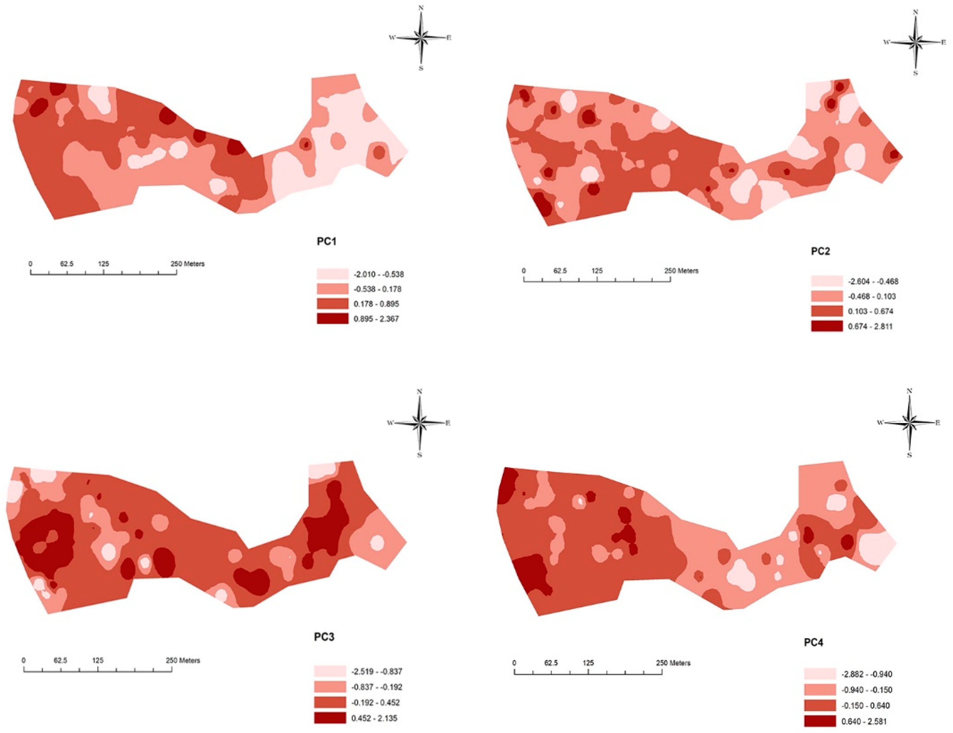
3.4. Principal Component Analysis

Table 2 showed that most of the studied soil properties were significantly correlated, and PCA was carried out to summarize and aggregate the variability in the studied ten variables. The number of the resulted principal components (PCs) must be equal to the number of the variables which were inserted into the analysis. PCs with eigen values more than 1 were kept for the final analysis, in which, according to Sharma [81], a PC with an eigen value more than 1 explains variance more than an individual attribute. Based on this principle, only the first four PCs described about 84% of the measured data total variability, as shown in Table 4. The OK method was carried out to interpolate the distribution maps of the 4 PCs as shown in Figure 4.
Principal component 1 (PC1) explained 33.28% of the total variability, and it was dominated by all the soil properties except soil C:N, C:P and N:P ratios. SOC, TP, C:N ratio and C:P ratio influenced the second principal component 2 (PC2), which explained 26.86% of total variability. While the third principle component 3 (PC3) explained 13.84 % of the total variability and was controlled by soil C:N and C:P ratios. Principal component 4 (PC4) explained 10.45 % of the variability and was affected by soil AN and AP.

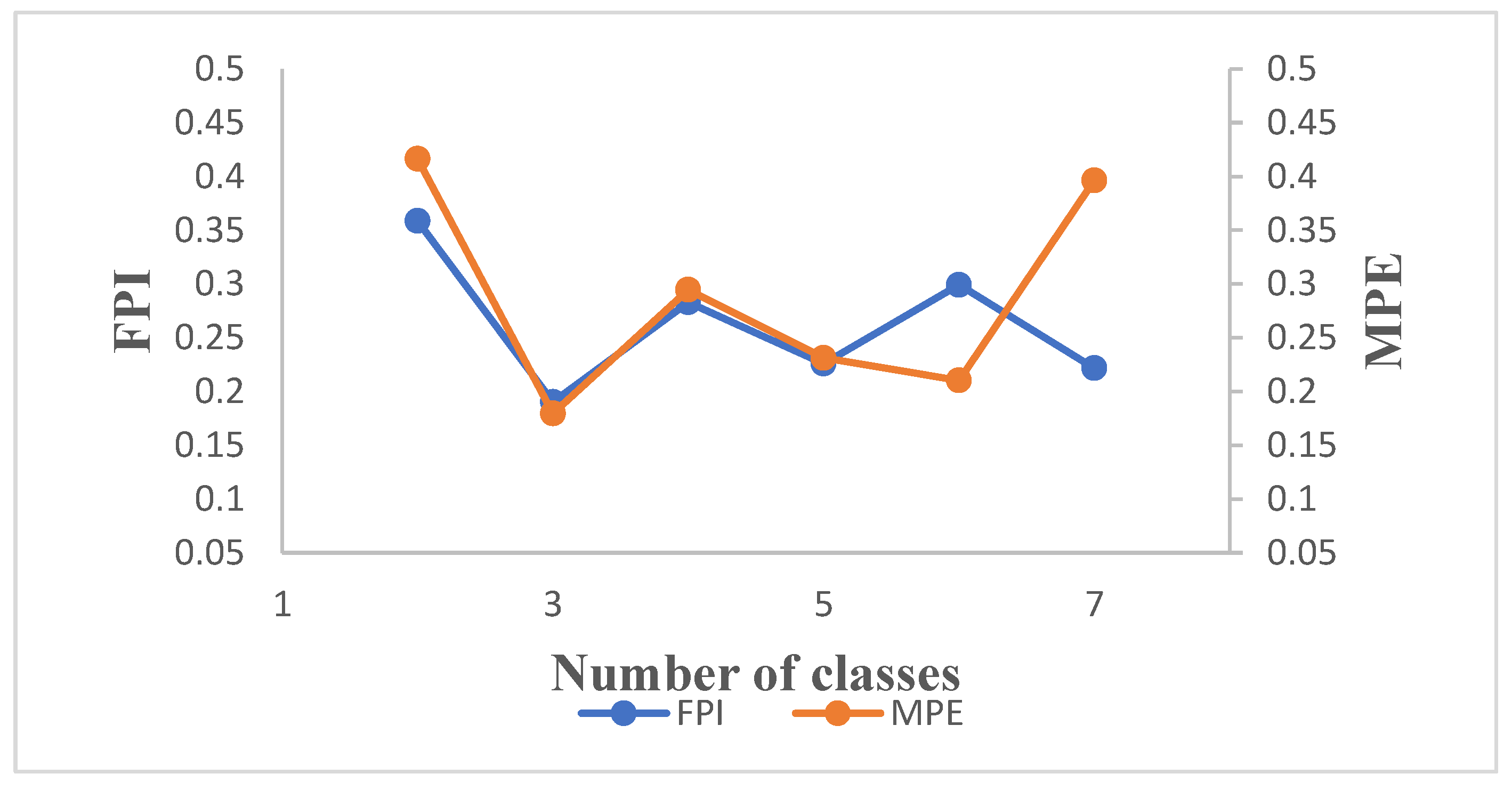
3.5. Management Zones Delineation Using Clustering Analysis

Scores of the first four PCs were inserted into FuzMe software to perform the fuzzy K-mean classification technique to cluster the four PCs into management zones (MZs). The two functions FPI and MPE were plotted versus the number of classes as shown in (Figure 5) to obtain the optimal number of MZs in the study area [82], in which, the minimum FPI met the minimum MPE against an optimum number of three clusters. The kriged map shown in (Figure 6) was describing three fertility management zones named as MZ1, MZ2 and MZ3. Analysis of variance was carried out using t-test to evaluate the efficiency of the spatial variability description of the studied soil properties over the delineated MZs by the combination of PCA and fuzzy k-means clustering. As shown in Table 5, the analysis of variance showed that the three delineated MZs were clearly diverse from each other. The same results were obtained by Tripathi et al. [83] and Shukla et al. [26].
Soil properties significantly varied across the three MZs. MZ2 had the highest soil pH value. The study area was in a dire need of nitrogen applications, in which AN concentrations were extremely low in MZ3, and very low in MZ1 and MZ2, while. While TN concentrations were medium, low and very low in MZ1, MZ2, and MZ3, respectively. Also, potassium application was needed in MZ2 and MZ3 which had medium concentrations of AK while MZ1 had high concentrations of it. For AP MZ1 and MZ2 had medium concentrations while MZ3 was high. SOC concentrations were low in MZ2 and very low in MZ1 and MZ3, so that it was very necessary to apply a considerable amount of organic matter to the study area, in which it was considered the main source of organic carbon which affects soil chemical, physical and biological properties influencing soil nutrients’ availability [37]. In addition, soil C:N and C:P ratios were very narrow in the study area which meant that soil organic matter was decomposing rapidly so that applying organic matter would be very useful to compensate for the decomposed organic matter. Therefore, the appropriate agricultural practices must be performed to improve soil organic matter content.
It is therefore very clear how much the importance of using site-specific land management for avoiding land degradation, as well as sustaining soil productivity, in the study area. Thus, cluster analysis is a suitable choice for identifying the study area MZs, and performing site-specific land management techniques will improve soil productivity, in which the average values of the studied soil properties within the MZs could be used as a reference for variable rate applications [36].

4. Conclusions

The studied soil properties’ coefficients of variation revealed high spatial variability and indicated that site-specific nutrient management techniques need to be performed in the study area. Soil AN, AP, TN and TP were positively correlated with SOC. Geostatistical tools were used to quantify the spatial variability of the studied soil properties. Geostatistical analysis revealed spherical and stable best-fit semi-variogram models for the studied soil properties. The studied soil properties were characterized by spatial heterogeneity, with spatial dependence ranging from weak to strong. Three MZs were delineated by performing PCA and fuzzy k-means clustering algorithms, and the variance analysis revealed soil fertility heterogeneity among the three zones. Future soil sampling processes may be optimized by using MZs information. The MZs map could be the guide for the precise management of nitrogen, phosphorous, potassium and organic carbon for the different zones in the study area to improve the soil chemical, physical and ecological properties to combat soil degradation, which was the principle of sustainable agriculture, in which the mean values of the studied soil properties in each of the three delineated zones could be used as a reference for applying variable rates of fertilizers.

Author Contributions

Conceptualization, M.S.M.; methodology, M.S.M. and R.-J.Y.; software, M.S.M., S.M.S. and R.-J.Y.; validation, M.S.M., S.M.S. and A.I.A.; formal analysis, M.S.M. and S.M.S.; investigation, M.S.M.; resources, M.L., P.L., J.J. and X.C.; data curation, M.S.M.; writing—original draft preparation, M.S.M.; writing—review and editing, M.S.M., M.L. and X.C.; visualization, M.S.M.; supervision, M.L.; project administration, M.L.; funding acquisition, M.L. and X.C.

Funding

This work was supported by Special Fund for Agro-scientific Research in the Public Interest (No. 201503121), China Agriculture Research System-Green Manure (No. CARS-22-G-10) and the Fundamental Research Funds for the Central Universities (No. KYYJ201702).

Acknowledgments

We greatly thank those persons who offered valuable helps in the soil sampling and laboratory analysis, namely J.S., D.Y., J.Z., J.H., and C.Z.

Conflicts of Interest

The authors declare no conflict of interest

References

  1. Safari, A.; Kavian, A.; Parsakhoo, A.; Saleh, I.; Jordán, A. Impact of different parts of skid trails on runoff and soil erosion in the Hyrcanian forest (northern Iran). Geoderma 2016, 263, 161–167. [Google Scholar] [CrossRef]
  2. Onojeghuo, A.O.; Blackburn, G.A.; Huang, J.; Kindred, D.; Huang, W. Applications of satellite ‘hyper-sensing’in Chinese agriculture: Challenges and opportunities. Int. J. Appl. Earth Obs. Geoinf. 2018, 64, 62–86. [Google Scholar] [CrossRef] [Green Version]
  3. Seutloali, K.E.; Beckedahl, H.R. Understanding the factors influencing rill erosion on roadcuts in the south eastern region of South Africa. Solid Earth 2015, 6, 633–641. [Google Scholar] [CrossRef] [Green Version]
  4. Borrelli, P.; Märker, M.; Schütt, B. Modelling post-tree-harvesting soil erosion and sediment deposition potential in the Turano River Basin (Italian Central Apennine). Land Degrad. Dev. 2015, 26, 356–366. [Google Scholar] [CrossRef]
  5. Taguas, E.; Guzmán, E.; Guzmán, G.; Vanwalleghem, T.; Gómez, J. Characteristics and importance of rill and gully erosion: A case study in a small catchment of a marginal olive grove. Cuad. De Investig. Geogr. 2015, 41, 107–126. [Google Scholar] [CrossRef] [Green Version]
  6. Rodrigo-Comino, J.; Seeger, M.; Senciales, J.; Ruiz-Sinoga, J.; Ries, J. Spatial and temporal variation of soil hydrological processes on steep slope vineyards (Ruwel-Mosel Valley, Gemany). Cuad. De Investig. Geogr. 2016, 42, 281–306. [Google Scholar] [CrossRef] [Green Version]
  7. Muñoz-Rojas, M.; Erickson, T.E.; Dixon, K.W.; Merritt, D.J. Soil quality indicators to assess functionality of restored soils in degraded semiarid ecosystems. Restor. Ecol. 2016, 24, S43–S52. [Google Scholar] [CrossRef]
  8. Ge, F.; Zhang, J.; Su, Z.; Nie, X. Response of changes in soil nutrients to soil erosion on a purple soil of cultivated sloping land. Acta Ecol. Sin. 2007, 27, 459–463. [Google Scholar] [CrossRef]
  9. Fitter, A.; Gilligan, C.; Hollingworth, K.; Kleczkowski, A.; Twyman, R.; Pitchford, J. Biodiversity and ecosystem function in soil. Funct. Ecol. 2005, 19, 369–377. [Google Scholar] [CrossRef] [Green Version]
  10. Thapa, G.; Yila, O.M. Farmers’ land management practices and status of agricultural land in the Jos Plateau, Nigeria. Land Degrad. Dev. 2012, 23, 263–277. [Google Scholar] [CrossRef]
  11. Zhao, G.; Mu, X.; Wen, Z.; Wang, F.; Gao, P. Soil erosion, conservation, and eco-environment changes in the Loess Plateau of China. Land Degrad. Dev. 2013, 24, 499–510. [Google Scholar] [CrossRef]
  12. Davatgar, N.; Neishabouri, M.; Sepaskhah, A. Delineation of site specific nutrient management zones for a paddy cultivated area based on soil fertility using fuzzy clustering. Geoderma 2012, 173, 111–118. [Google Scholar] [CrossRef]
  13. Ferguson, R.B.; Hergert, G.W.; Schepers, J.; Gotway, C.; Cahoon, J.; Peterson, T. Site-specific nitrogen management of irrigated maize: Yield and soil residual nitrate effects. Soil Sci. Soc. Am. J. 2002, 66, 544–553. [Google Scholar] [CrossRef]
  14. Abd-Elmabod, S.K.; Ali, R.R.; Anaya-Romero, M.; de la Rosa, D. Evaluating soil contamination risks by using MicroLEIS DSS in El-Fayoum Province, Egypt. In Proceedings of the 2010 2nd International Conference on Chemical, Biological and Environmental Engineering, Cairo, Egypt, 2–4 November 2010; pp. 1–5. [Google Scholar]
  15. Mansour, H.A.; Abd-Elmabod, S.K.; Engel, B. Adaptation of modeling to the irrigation system and water management for corn growth and yield. Plant Arch. 2019, 19, 644–651. [Google Scholar]
  16. Far, S.T.; Rezaei-Moghaddam, K. Impacts of the precision agricultural technologies in Iran: An analysis experts’ perception & their determinants. Inf. Process. Agric. 2018, 5, 173–184. [Google Scholar]
  17. Oliver, M.E.A. An overview of precision agriculture. In Precision Agriculture for Sustainability and Environmental Protection; Routledge: Abingdon, UK, 2013; pp. 21–37. [Google Scholar]
  18. Buttafuoco, G.; Castrignanò, A.; Cucci, G.; Lacolla, G.; Lucà, F. Geostatistical modelling of within-field soil and yield variability for management zones delineation: A case study in a durum wheat field. Precis. Agric. 2017, 18, 37–58. [Google Scholar] [CrossRef]
  19. Mansour, H.A.; Jiandong, H.; Hongjuan, R.; Kheiry, A.N.; Abd-Elmabod, S.K. Influence of using automatic irrigation system and organic fertilizer treatments on faba bean water productivity. Int. J. 2019, 17, 250–259. [Google Scholar] [CrossRef]
  20. Castrignanò, A.; Buttafuoco, G.; Quarto, R.; Parisi, D.; Rossel, R.V.; Terribile, F.; Langella, G.; Venezia, A. A geostatistical sensor data fusion approach for delineating homogeneous management zones in Precision Agriculture. Catena 2018, 167, 293–304. [Google Scholar] [CrossRef]
  21. Mueller, T.; Hartsock, N.; Stombaugh, T.; Shearer, S.; Cornelius, P.; Barnhisel, R. Soil electrical conductivity map variability in limestone soils overlain by loess. Agron. J. 2003, 95, 496–507. [Google Scholar] [CrossRef]
  22. Saito, H.; McKenna, S.A.; Zimmerman, D.; Coburn, T.C. Geostatistical interpolation of object counts collected from multiple strip transects: Ordinary kriging versus finite domain kriging. Stoch. Environ. Res. Risk Assess. 2005, 19, 71–85. [Google Scholar] [CrossRef]
  23. Shaddad, S.M. Geostatistics and Proximal Soil Sensing for Sustainable Agriculture. In Sustainability of Agricultural Environment in Egypt: Part I; Springer: Chim, Switzerland, 2018; pp. 255–271. [Google Scholar]
  24. Brevik, E.C.; Calzolari, C.; Miller, B.A.; Pereira, P.; Kabala, C.; Baumgarten, A.; Jordán, A. Soil mapping, classification, and pedologic modeling: History and future directions. Geoderma 2016, 264, 256–274. [Google Scholar] [CrossRef]
  25. Bogunovic, I.; Pereira, P.; Brevik, E.C. Spatial distribution of soil chemical properties in an organic farm in Croatia. Sci. Total Environ. 2017, 584, 535–545. [Google Scholar] [CrossRef] [PubMed] [Green Version]
  26. Shukla, A.K.; Sinha, N.K.; Tiwari, P.K.; Prakash, C.; Behera, S.K.; Lenka, N.K.; Singh, V.K.; Dwivedi, B.S.; Majumdar, K.; Kumar, A. Spatial distribution and management zones for sulphur and micronutrients in Shiwalik Himalayan Region of India. Land Degrad. Dev. 2017, 28, 959–969. [Google Scholar] [CrossRef]
  27. Abd-Elmabod, S.K.; Fitch, A.C.; Zhang, Z.; Ali, R.R.; Jones, L. Rapid urbanisation threatens fertile agricultural land and soil carbon in the Nile delta. J. Environ. Manag. 2019, 252, 109668. [Google Scholar] [CrossRef] [PubMed]
  28. Abd-Elmabod, S.K.; Jordán, A.; Fleskens, L.; Phillips, J.D.; Muñoz-Rojas, M.; van der Ploeg, M.; Anaya-Romero, M.; El-Ashry, S.; de la Rosa, D. Modeling agricultural suitability along soil transects under current conditions and improved scenario of soil factors. In Soil Mapping and Process Modeling for Sustainable Land Use Management; Elsevier: Amsterdam, The Netherland, 2017; pp. 193–219. [Google Scholar]
  29. Abd-Elmabod, S.K.; Bakr, N.; Muñoz-Rojas, M.; Pereira, P.; Zhang, Z.; Cerdà, A.; Jordán, A.; Mansour, H.; De la Rosa, D.; Jones, L. Assessment of soil suitability for improvement of soil factors and agricultural management. Sustainability 2019, 11, 1588. [Google Scholar] [CrossRef] [Green Version]
  30. Yao, R.-J.; Yang, J.-S.; Zhang, T.-J.; Gao, P.; Wang, X.-P.; Hong, L.-Z.; Wang, M.-W. Determination of site-specific management zones using soil physico-chemical properties and crop yields in coastal reclaimed farmland. Geoderma 2014, 232, 381–393. [Google Scholar] [CrossRef]
  31. Ferguson, R.; Lark, R.; Slater, G. Approaches to management zone definition for use of nitrification inhibitors. Soil Sci. Soc. Am. J. 2003, 67, 937–947. [Google Scholar] [CrossRef]
  32. Khosla, R.; Shaver, T. Zoning in on nitrogen needs. Colo. State Univ. Agron. Newsl. 2001, 21, 24–26. [Google Scholar]
  33. Khosla, R.; Alley, M. Soil-specific nitrogen management on mid-Atlantic coastal plain soils. Better Crops 1999, 83, 6–7. [Google Scholar]
  34. Fleming, K.; Westfall, D.; Wiens, D.; Brodahl, M. Evaluating farmer defined management zone maps for variable rate fertilizer application. Precis. Agric. 2000, 2, 201–215. [Google Scholar] [CrossRef]
  35. Mzuku, M.; Khosla, R.; Reich, R.; Inman, D.; Smith, F.; MacDonald, L. Spatial variability of measured soil properties across site-specific management zones. Soil Sci. Soc. Am. J. 2005, 69, 1572–1579. [Google Scholar] [CrossRef] [Green Version]
  36. Nawar, S.; Corstanje, R.; Halcro, G.; Mulla, D.; Mouazen, A.M. Delineation of soil management zones for variable-rate fertilization: A review. In Advances in Agronomy; Elsevier: San Diego, CA, USA, 2017; Volume 143, pp. 175–245. [Google Scholar]
  37. Behera, S.K.; Mathur, R.K.; Shukla, A.K.; Suresh, K.; Prakash, C. Spatial variability of soil properties and delineation of soil management zones of oil palm plantations grown in a hot and humid tropical region of southern India. Catena 2018, 165, 251–259. [Google Scholar] [CrossRef]
  38. Mallarino, A.; Oyarzabal, E.; Hinz, P. Interpreting within-field relationships between crop yields and soil and plant variables using factor analysis. Precis. Agric. 1999, 1, 15–25. [Google Scholar] [CrossRef]
  39. Goovaerts, P. Geostatistics for Natural Resources Evaluation; Oxford University Press: Oxford, NY, USA, 1997. [Google Scholar]
  40. Li, Y.; Shi, Z.; Li, F.; Li, H.-Y. Delineation of site-specific management zones using fuzzy clustering analysis in a coastal saline land. Comput. Electron. Agric. 2007, 56, 174–186. [Google Scholar] [CrossRef]
  41. Tisdale, S.L.; Nelson, W.L.; Beaton, J.D. Soil Fertility and Fertilizers; Collier Macmillan Publishers: London, UK, 1985. [Google Scholar]
  42. Chapin, F.S. Effects of plant traits on ecosystem and regional processes: A conceptual framework for predicting the consequences of global change. Ann. Bot. 2003, 91, 455–463. [Google Scholar] [CrossRef] [PubMed] [Green Version]
  43. Jiménez, J.J.; Lorenz, K.; Lal, R. Organic carbon and nitrogen in soil particle-size aggregates under dry tropical forests from Guanacaste, Costa Rica—Implications for within-site soil organic carbon stabilization. Catena 2011, 86, 178–191. [Google Scholar] [CrossRef] [Green Version]
  44. Liu, Z.P.; Shao, M.A.; Wang, Y.Q. Spatial patterns of soil total nitrogen and soil total phosphorus across the entire Loess Plateau region of China. Geoderma 2013, 197, 67–78. [Google Scholar] [CrossRef]
  45. Gao, Y.; He, N.; Yu, G.; Chen, W.; Wang, Q. Long-term effects of different land use types on C, N, and P stoichiometry and storage in subtropical ecosystems: A case study in China. Ecol. Eng. 2014, 67, 171–181. [Google Scholar] [CrossRef]
  46. Lal, R. Soil carbon sequestration impacts on global climate change and food security. Science 2004, 304, 1623–1627. [Google Scholar] [CrossRef] [Green Version]
  47. IPCC. The physical science basis. In Contribution of Working Group I to the Fourth Assessment Report of the Intergovernmental Panel on Climate Change, Cambridge, UK; Cambridge University Press: Cambridge, UK, 2007; pp. 337–383. [Google Scholar]
  48. Sardans, J.; Peñuelas, J. The role of plants in the effects of global change on nutrient availability and stoichiometry in the plant-soil system. Plant Physiol. 2012, 160, 1741–1761. [Google Scholar] [CrossRef] [Green Version]
  49. Paul, E.A. Soil Microbiology, Ecology and Biochemistry; Academic press: London/Oxford, UK; San Diego, CA/Waltham, MA, USA, 2014. [Google Scholar]
  50. Bui, E.N.; Henderson, B.L. C: N: P stoichiometry in Australian soils with respect to vegetation and environmental factors. Plant Soil 2013, 373, 553–568. [Google Scholar] [CrossRef]
  51. Peñuelas, J.; Sardans, J.; Rivas-ubach, A.; Janssens, I.A. The human-induced imbalance between C, N and P in Earth’s life system. Glob. Chang. Biol. 2012, 18, 3–6. [Google Scholar] [CrossRef]
  52. Tian, H.; Chen, G.; Zhang, C.; Melillo, J.M.; Hall, C.A. Pattern and variation of C: N: P ratios in China’s soils: A synthesis of observational data. Biogeochemistry 2010, 98, 139–151. [Google Scholar] [CrossRef]
  53. Jackson, M.L. Soil Chemical Analysis; Indian, Ed.; Prentice Hall of India: New Delhi, India, 1973. [Google Scholar]
  54. Walkley, A.; Black, I.A. An examination of the Degtjareff method for determining soil organic matter, and a proposed modification of the chromic acid titration method. Soil Sci. 1934, 37, 29–38. [Google Scholar] [CrossRef]
  55. Bremner, J. Determination of nitrogen in soil by the Kjeldahl method. J. Agric. Sci. 1960, 55, 11–33. [Google Scholar] [CrossRef]
  56. Alexander, T.; Robertson, A. Ascorbic acid as a reductant for total phosphorus determination in soils. Can. J. Soil Sci. 1968, 48, 217–218. [Google Scholar] [CrossRef]
  57. Chapman, H.D.; Pratt, P.F. Methods of analysis for soils, plants and waters. Soil Sci. 1962, 93, 68. [Google Scholar] [CrossRef] [Green Version]
  58. Olsen, S.R. Estimation of available phosphorus in soils by extraction with sodium bicarbonate. US Dep. Agric. Circ. 1954, 939, 1–19. [Google Scholar]
  59. Piper, C.S. Soil and plant analysis: A laboratory manual of methods for the examination of soils and the determination of the inorganic constituents of plants; Hans Publishers: Bombay, India, 1966. [Google Scholar]
  60. Gee, G.W.; Bauder, J.W. Particle size analysis. In Methods of Soil Analysis: Part I, 2nd ed.; Klute, A., Ed.; Soil Science Society of America, American Society of Agronomy: Madison, WI, USA, 1986; Volume 9, pp. 383–411. [Google Scholar]
  61. Goovaerts, P. Geostatistical tools for characterizing the spatial variability of microbiological and physico-chemical soil properties. Biol. Fertil. Soils 1998, 27, 315–334. [Google Scholar] [CrossRef] [Green Version]
  62. Meul, M.; Van Meirvenne, M. Kriging soil texture under different types of nonstationarity. Geoderma 2003, 112, 217–233. [Google Scholar] [CrossRef]
  63. Triantafilis, J.; Odeh, I.; McBratney, A. Five geostatistical models to predict soil salinity from electromagnetic induction data across irrigated cotton. Soil Sci. Soc. Am. J. 2001, 65, 869–878. [Google Scholar] [CrossRef]
  64. Schepers, A.R.; Shanahan, J.F.; Liebig, M.A.; Schepers, J.S.; Johnson, S.H.; Luchiari, A. Appropriateness of management zones for characterizing spatial variability of soil properties and irrigated corn yields across years. Agron. J. 2004, 96, 195–203. [Google Scholar] [CrossRef] [Green Version]
  65. Minasny, B.; McBratney, A.B. A conditioned Latin hypercube method for sampling in the presence of ancillary information. Comput. Geosci. 2006, 32, 1378–1388. [Google Scholar] [CrossRef]
  66. Grunwald, S.; Osborne, T.; Reddy, K. Temporal trajectories of phosphorus and pedo-patterns mapped in Water Conservation Area 2, Everglades, Florida, USA. Geoderma 2008, 146, 1–13. [Google Scholar] [CrossRef]
  67. Boydell, B.; McBratney, A. Identifying potential within-field management zones from cotton-yield estimates. Precis. Agric. 2002, 3, 9–23. [Google Scholar] [CrossRef]
  68. Soil Survey Office of China. China Soil Survey Technique; Agricultural Press: Beijing, China, 1992. (In Chinese) [Google Scholar]
  69. Zhao, F.; Sun, J.; Ren, C.; Kang, D.; Deng, J.; Han, X.; Yang, G.; Feng, Y.; Ren, G. Land use change influences soil C, N, and P stoichiometry under ‘Grain-to-Green Program’in China. Sci. Rep. 2015, 5, 10195. [Google Scholar]
  70. Wang, X.; Ma, X.; Yan, Y. Effects of soil C: N: P stoichiometry on biomass allocation in the alpine and arid steppe systems. Ecol. Evol. 2017, 7, 1354–1362. [Google Scholar] [CrossRef]
  71. Wang, X.Z.; Liu, G.S.; Hu, H.C.; Wang, Z.H.; Liu, Q.H.; Liu, X.F.; Hao, W.H.; Li, Y.T. Determination of management zones for a tobacco field based on soil fertility. Comput. Electron. Agric. 2009, 65, 168–175. [Google Scholar]
  72. Karaman, M.; Ersahin, S.; Durak, A. Spatial variability of available phosphorus and site specific P fertilizer recommendations in a wheat field. In Plant Nutrition; Springer: Dordrecht, The Netherlands, 2001; pp. 876–877. [Google Scholar]
  73. Jakobsen, B.H. Soil spatial variability: Proceedings of a workshop of the ISSS and the SSSA Las Vegas, USA 30 november-1 december 1984/DR Nielsen and J. Bouma (Eds.). Geogr. Tidsskr. 1985. Available online: https://tidsskrift.dk/geografisktidsskrift/article/view/44191 (accessed on 16 October 2019).
  74. Ouyang, S.; Xiang, W.; Gou, M.; Lei, P.; Chen, L.; Deng, X. Variations in soil carbon, nitrogen, phosphorus and stoichiometry along forest succession in southern China. Phys. Chem. Earth 2018, 103, 28–34. [Google Scholar] [CrossRef] [Green Version]
  75. López-Granados, F.; Jurado-Expósito, M.; Atenciano, S.; García-Ferrer, A.; de la Orden, M.S.; García-Torres, L. Spatial variability of agricultural soil parameters in southern Spain. Plant Soil 2002, 246, 97–105. [Google Scholar] [CrossRef]
  76. Liu, G.; Wang, X.; Zhang, Z.; Zhang, C. Spatial variability of soil properties in a tobacco field of central China. Soil Sci. 2008, 173, 659–667. [Google Scholar]
  77. Jiang, H.; Liu, G.; Wang, X.; Song, W.; Zhang, R.; Zhang, R.; Hu, H.; Li, L. Delineation of site-specific management zones based on soil properties for a hillside field in central China. Arch. Agron. Soil Sci. 2012, 58, 1075–1090. [Google Scholar] [CrossRef]
  78. Cambardella, C.A.; Moorman, T.B.; Parkin, T.; Karlen, D.; Novak, J.; Turco, R.; Konopka, A. Field-scale variability of soil properties in central Iowa soils. Soil Sci. Soc. Am. J. 1994, 58, 1501–1511. [Google Scholar] [CrossRef]
  79. Kerry, R.; Oliver, M. Average variograms to guide soil sampling. Int. J. Appl. Earth Obs. Geoinf. 2004, 5, 307–325. [Google Scholar] [CrossRef]
  80. Shaddad, S.; Buttafuoco, G.; Elrys, A.; Castrignanò, A. Site-specific management of salt affected soils: A case study from Egypt. Sci. Total Environ. 2019, 688, 153–161. [Google Scholar] [CrossRef]
  81. Sharma, S. Applied Multivariate Techniques; Wiley: New York, NY, USA, 1996. [Google Scholar]
  82. Fridgen, J.J.; Kitchen, N.R.; Sudduth, K.A.; Drummond, S.T.; Wiebold, W.J.; Fraisse, C.W. Management zone analyst (MZA): Software for subfield management zone delineation. Agron. J. 2004, 96, 100–108. [Google Scholar] [CrossRef]
  83. Tripathi, R.; Nayak, A.; Shahid, M.; Lal, B.; Gautam, P.; Raja, R.; Mohanty, S.; Kumar, A.; Panda, B.; Sahoo, R. Delineation of soil management zones for a rice cultivated area in eastern India using fuzzy clustering. Catena 2015, 133, 128–136. [Google Scholar] [CrossRef]
Figure 1. Location of the study area (Jianyang, Sichuan, China) with sampling points
Sustainability 11 07084 g001
Figure 2. Experimental semi-variograms and fitted models for AN, AP, AK, SOC, TN, TP, C:N, C:P, N:P ratios and pH.
Sustainability 11 07084 g002
Figure 3. Soil properties ordinary kriged distribution maps of the study area.
Sustainability 11 07084 g003
Figure 4. Kriged maps of the first four principal components.
Sustainability 11 07084 g004
Figure 5. Fuzzy performance index (FPI) and modified partition entropy (MPE) calculated for delineating the optimum number of clusters for the study area.
Sustainability 11 07084 g005
Figure 6. Soil management zones of the study area.
Sustainability 11 07084 g006
Table 1. Descriptive statistics for the studied soil properties.
Parameter *MinimumMaximumMeanMedianSDSkewnessKurtosisCV (%)
AN13.1349.8835.4235.887.28−0.490.2820.55
AK100.00210.00147.10145.0022.800.500.3915.50
AP5.8038.2917.0215.717.791.130.9145.75
pH7.858.318.138.130.09−0.330.241.13
TP0.541.110.830.820.130.16−0.5915.59
TN0.621.430.980.980.170.190.1016.92
SOC4.4114.479.589.682.22−0.26−0.4623.20
CN4.2814.839.839.861.89−0.380.6419.27
CP4.4620.4811.6511.822.800.081.0024.00
NP0.771.681.191.160.180.430.0715.50
* AN, available nitrogen (mg/kg); AK, available potassium (mg/kg); AP, available phosphorous (mg/kg); TP, total phosphorus (g/kg); TN, total nitrogen (g/kg); SOC, soil organic carbon; CN, carbon nitrogen ratio; CP, carbon phosphorus ratio; NP, nitrogen phosphorus ratio; SD: standard deviation; CV: coefficient of variation.
Table 2. Pearson’s correlation coefficient values showing relationship among the study area soil properties.
.ANAKAPpHTPTNSOCCNCPNP
AN1.000
AK0.376 **1.000
AP0.1090.450 **1.000
pH−0.271 **−0.427 **−0.399 **1.000
TP0.500 **0.372 **0.372 **−0.283 **1.000
TN0.546 **0.536 **0.342 **−0.311 **0.562 **1.000
SOC0.357 **0.1930.238 *−0.1470.274 **0.572 **1.000
CN−0.026−0.207 *−0.0210.087−0.164−0.1670.705 **1.000
CP0.025−0.043−0.0300.035−0.380 **0.1850.768 **0.770 **1.000
NP0.1060.206 *−0.026−0.047−0.398 **0.520 **0.336 **−0.0300.600 **1.000
AN: available nitrogen; SOC: soil organic carbon; AP: available phosphorous; AK: available potassium; TP: total phosphorus; C:N:C:Nratio; C:P:C:P ratio; N:P: N:P ratio. ** Correlation is significant at the 0.01 level (2-tailed). * Correlation is significant at the 0.05 level (2-tailed).
Table 3. The study area soil properties Semi-variogram parameters.
VariableModelNuggetPartial SillSillNugget/SillSDCRange (m)MEMSSE
SOCStable3.9503.0507.0000.5643Moderate679.4−0.0131.046
TNSpherical0.0210.0080.0290.7241Moderate278.2−0.0041.003
TPStable0.0150.0010.0160.9375Weak134.00.0011.019
pHSpherical0.0070.0010.0080.8750Weak679.40.0031.064
APSpherical0.1580.0570.2150.7349Moderate289.3−0.0661.031
ANStable0.00049.62049.6200.0000Strong116.1−0.0081.027
AKSpherical202.500292.870495.3700.4088Moderate48.7−0.6911.056
NPSpherical0.0300.0030.0330.9091Weak138.00.0301.135
CPSpherical6.4762.8259.3010.6963Moderate679.4−0.0311.111
CNSpherical2.8791.3504.2290.6808Moderate600.0−0.0091.026
AN: available nitrogen; SOC: soil organic carbon; AP: available phosphorous; AK: available potassium; TP: total phosphorus; C:N: C:N ratio; C:P::C:P ratio; N:P: N:P ratio; SDC: spatial dependency class; MSSE: mean square standardized error; ME: mean error.
Table 4. Principal component analysis of soil properties and loading coefficient for the first four principal components.
Principal ComponentEigen ValuesComponent Loading (%)Cumulative Loading (%)
13.32833.28533.285
22.68626.86460.149
31.38413.84273.991
41.04510.45084.441
50.6776.77191.212
60.4764.76295.974
70.3733.72999.703
80.0180.18299.885
90.0070.07399.957
100.0040.043100.000
Principal component loading for each variable
ANAKAPpHTPTNSOCC:N ratioC:P ratioN:P ratio
PC10.6510.6700.532−0.5180.5600.8740.7350.1390.3460.386
PC2−0.185−0.337−0.2670.287−0.573−0.0960.5800.7860.9290.481
PC30.073−0.2260.1700.0050.459−0.2620.2990.571−0.032−0.776
PC40.500−0.221−0.6020.4770.2680.2440.085−0.104−0.0850.019
Table 5. The mean values of soil properties in the three management zones.
Management ZonesNo. of PointsANAKAPpHTPTNSOCC:N RatioC:P RatioN:P Ratio
13139.36 a155.65 a15.31 b8.11 ab0.84 a1.09 a9.03 b8.23 c10.98 b1.32 a
24436.64 a141.77 b15.37 b8.15 a0.85 a0.96 b10.66 a11.09 a12.63a1.14 b
32528.39 b145.88 ab22.04 a8.09 b0.79 a0.87 c8.37 b9.57 b10.74 b1.11 b
Different letters (a, b and c) within each column indicate a significant difference between the management zones at the 0.05 level.

