Article

Effects of Landscape Development Intensity on River Water Quality in Urbanized Areas

1
Joint Laboratory of Ecological Urban Design (Research Centre for Land Ecological Planning, Design and Environmental Effects; International Joint Research Centre of Urban-Rural Ecological Planning and Design), College of Architecture and Urban Planning, Tongji University, Shanghai 200092, China
2
Department of Landscape Studies, College of Architecture and Urban Planning, Tongji University, Shanghai 200092, China
3
International Center of Urban & Rural Ecological Planning and Design Research, Key Laboratory of Ecology and Energy-Saving Study of Dense Habitat, Ministry of Education, Shanghai 200092, China
4
Department of Urban Planning, College of Architecture and Urban Planning, Tongji University, Shanghai 200092, China
*
Authors to whom correspondence should be addressed.
Sustainability 2019, 11(24), 7120; https://doi.org/10.3390/su11247120
Submission received: 10 October 2019 / Revised: 21 November 2019 / Accepted: 9 December 2019 / Published: 12 December 2019
(This article belongs to the Section Sustainable Urban and Rural Development)

Abstract

:
Urban development and human activities have greatly changed the appearance of urban landscapes, and also affect urban river water environments. Rapidly urbanized regions in China face particularly severe pressures and challenges in alleviating degradation of river water quality. Information is needed on which indexes of landscape development intensity in rapidly-urbanized areas are the key factors affecting the quality of river water environments, and how these factors affect water quality. In order to answer these questions, this research selected six indexes belonging to three dimensions for landscape development intensity evaluation. Based on five water quality parameters of 20 rivers and the land use data of 20 small watersheds of Liangjiang New Area, Chongqing, China in 2014, this research explored the correlation between the landscape development intensity indexes and river water quality through redundancy analysis. We found that the impervious surface rate and the land average fixed asset investment are the key indexes to affect river water quality. Regulating the corresponding indexes at the urban planning and design level, as well as the decision making level, can effectively achieve the goal of improving urban river water quality. The conclusions inspire strategies in planning and design, and are helpful for government decision making to effectively protect river water environment in rapidly urbanized areas in the developing countries.

1. Introduction

Rivers in the city, serving as reliable surface water sources, are important natural geographical elements and ecological corridors in urban landscape, beneficial to public health and ecological environment [1,2,3]. The degradation of river water quality of watershed has become a global environmental issue in recent years [4,5], which is proved to be attributed to many natural and anthropogenic factors in watershed landscapes [6,7,8]. Studies have shown that the condition of urban rivers is strongly influenced by human activities, especially land use and cover changes in the process of urbanization within the surrounding landscape [9,10,11,12,13,14]. Under the influence of urbanization, non-point source pollution caused by rainwater runoff has become one of the important reasons for the deterioration of urban water environment [15,16]. Water quality parameters such as total soluble solid (TSS), chemical oxygen demand (CODMN), total nitrogen (TN), ammonia nitrogen (NH3+-N), and total phosphorus (TP) are representative pollutant parameters, which describe the physical and chemical characteristics of water bodies, have attracted more attention in water quality studies in urbanized areas [17,18,19,20,21,22].
Some studies focus on the spatial effects of human activities on water quality, and the effects of landscape pattern and structure of land use in adjacent water bodies or of the reservoirs on water quality are studied [23,24,25]. Extensive studies highlight the impacts of different land use types on water quality, such as areal proportion [26,27], topographic characteristics [28,29,30], multi-spatial scales [31,32], and seasonal and temporal changes [33,34]. However, some scholars argued that even with similar or same land use types and proportions, different land use intensities may result in a wide range of water quality [35,36]; only using the quantitative proportion of land use in the watershed to explain the water quality performance will often lead to different findings [10,11,12,13,37,38].
Therefore, some scholars introduced the concept of “intensity” into the study of the relationship between human activities interference and water quality, defining “land use intensity” as the levels of socio-economic inputs and human activities of the land use by unit area and time [37,39,40]. Land use intensity indicators such as land inputs (e.g., fertilizer use and livestock feeding) and land disturbance (e.g., vegetation removal or planting) are believed to be better predictors of human impacts than land use proportion alone [40], and can be directly applied to the study of the correlation with water quality [37,41].
In rapidly urbanized areas, the development of human beings on the landscape through land use changes has always been a concern and considered as a threat to our environment [42,43]. Landscape development is a kind of human disturbance to the environment and is manifested as human-dominated land uses [44]. The more developed a landscape, the greater the intensity of human impacts [45]. Brown et al. [45] proposed the “landscape development intensity index”, which is used as a gauge of human activity based on a development intensity measure derived from nonrenewable energy use in the surrounding landscape, and uses LDI coefficient to express the calculated emergy values after normalization [46,47,48]. This method is a good attempt to quantify anthropogenic influence based on primary indices of anthropogenic influences [46]. It has been directly used to evaluate the health of wetland ecosystem [44,49,50]. Some studies have developed the method by modifying the LDI coefficient and combining with other measure indexes, such as landscape matrix, forest cover, and road density to evaluate the current condition of wetlands [9,51,52].
However, the indicators used in existing studies to characterize the development intensity of land use or landscape of agricultural land and grassland [39], as well as the emergy approach for wetland, are applicable to areas characterized by low population densities. These indicators are not able to well represent the comprehensive impact of human activities on water quality through landscape changes in cities, the majority of which are surrounded by areas of high population density and development. What is more, the values of LDI index proposed by Brown et al. were affected by both area of various land use types and the LDI coefficient within the assessed regions [52]. In urban areas with complex land use and frequent human activities, it is challenging to modify the LDI coefficient and determine the LDI index value. Also, instead of accounting for individual causal agents directly, the LDI index represents the combined effects of many factors [46]. Thus a more direct and easy approach needs to be applied.
Given the studies cited previously, this research considered that it is feasible to use the index method to describe and evaluate the landscape development intensity in urbanized areas, and was based on the main idea that there are indexes of landscape development intensity as key factors affecting the river water quality in rapidly urbanized areas. This research draws on the concept of “landscape development intensity” (LDI) proposed by Brown et al. [45] to describe the disturbance degree of human activities to urban landscape, and extends its application field to urban construction areas.
In urban construction areas, the impact of human interference on environment occurs through development and construction behavior and social and economic factors, and finally acts on urban natural environment. In this research field, some scholars have evaluated the level of landscape or land development through the concept and indicators of “Urban land development intensity (ULDI)”. ULDI within a certain urban area evaluates the land relative development degree and its cumulative carrying density under the condition of regional environmental carrying capacity [53]. Evaluation aspects of ULDI includes political and economic, cultural and technological, as well as natural and spatial [54,55,56,57]. Specific indicators such as: urban population density, ratio of total investment in fixed assets to urban areas, area of built district as percentage to urban areas, transit network density, green areas per capita in urban built district, and cultivated area per capita are used in the studies to represent and evaluate urban development intensity [58,59,60,61,62,63], which provide good references for characterizing the urban landscape development intensity in this research.
To quantify the landscape development intensity in rapid urbanized areas, the LDI evaluation in this research was designed by selecting appropriate indexes that are more easily accessible in rapidly urbanized areas on the impact of human interference on water quality, with reference to previously developed indexes. By studying 20 watersheds in Liangjiang New Area, Chongqing, China, we calculated six landscape development intensity indexes and five water quality parameters and studied the correlations between them. Understanding the relationships between landscape development intensity and water quality is important for watershed planning and management and maintenance of ecosystem structure and functions in watersheds.

2. Materials and Methods
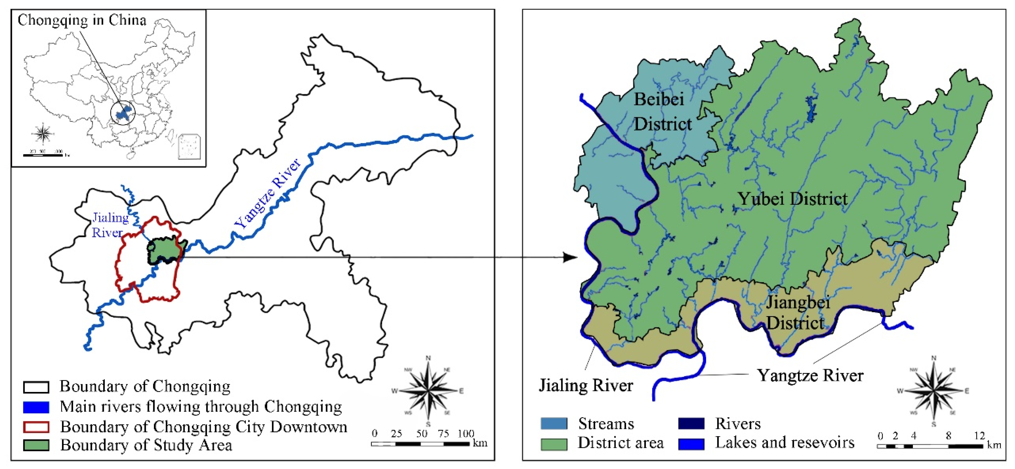
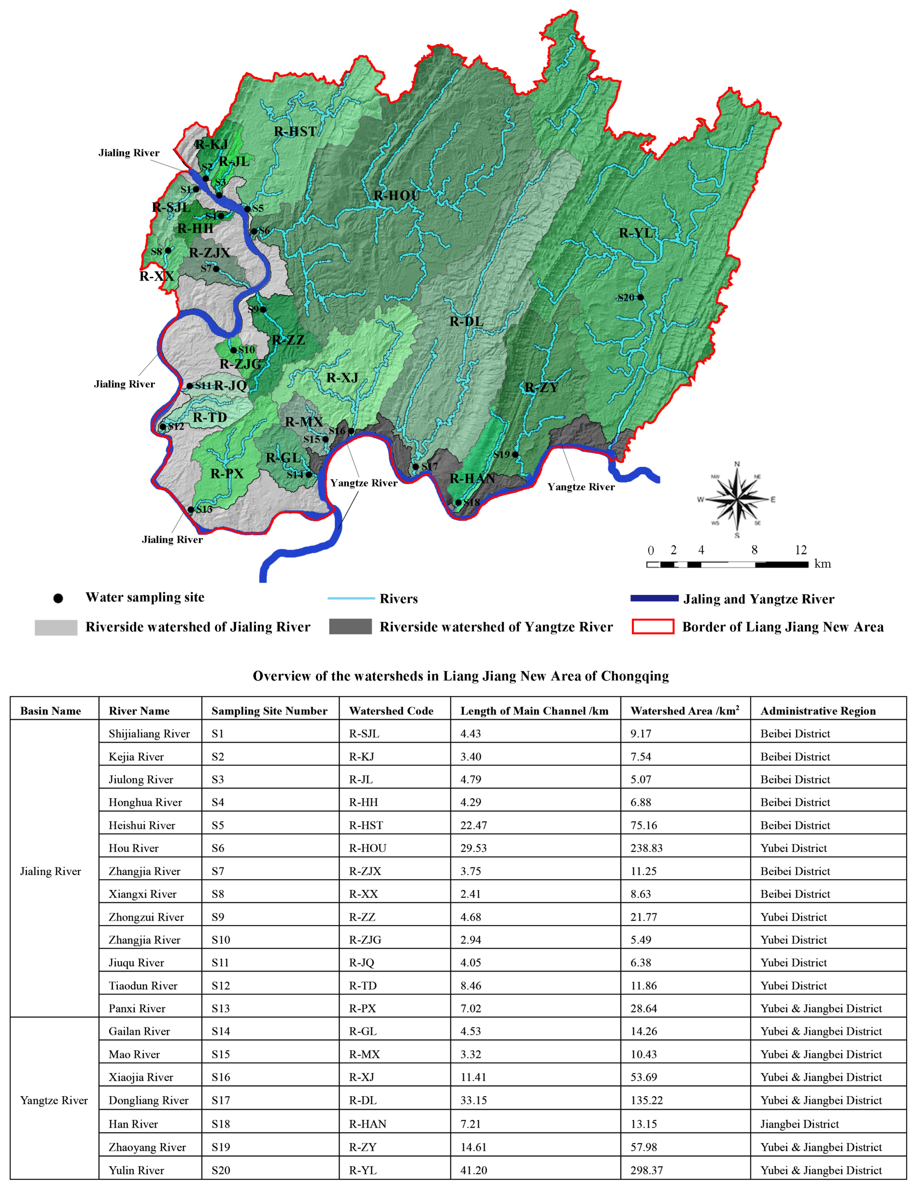
2.1. Study Area

Chongqing is located in southwestern China, the upper reaches of the Yangtze River, with mountains and hills of complex terrain. Rich in waters and rivers, the Chongqing section of the Three Gorges reservoir area covers 85.6% of the area of the Three Gorges reservoir area which means an important ecological location. Therefore, the stability of the water environment in Chongqing has great ecological and strategic significance for the maintenance of the ecological function of the Three Gorges reservoir area.
Liangjiang New Area in Chongqing, which was formally established in 2010, is a state-level development and new district, which is located in the Chongqing section of Three Gorges reservoir area, including three administrative districts, namely Jiangbei district, Yubei District, and Beibei district [64] (Figure 1). Liangjiang New Area is in the stage of accelerating urbanization. In 2014, the registered population was 1.5544 million and the resident population was 2.2446 million. In 2014, the regional GDP reached 186.1 billion yuan, with 15% year-on-year growth, accounting for more than 13% of the city [65].
Due to industrial development, urban space expansion, excessive construction intensity around rivers and lakes in built-up areas, as well as the population aggregation and land intensification caused by land shortage in mountainous cities, the local water system structure in urban construction areas is disordered, which aggravates the problems of overall water environment of rivers and lakes. The degradation of river water quality in the Liangjiang New Area of Chongqing affects the health of the regional water environment and further threatens the stability of the water ecological environment in the Three Gorges reservoir area.

2.2. Data Processing

2.2.1. Water Quality Parameters

In this research, 20 major rivers in Liangjiang New Area were studied. A total of 20 water quality sampling sites are selected where the estuary and tributaries of each main stream flow into the main stream mouth, which is convenient for traffic and less affected by point source pollution. The natural catchment unit is divided into 20 small watersheds by dividing the outlet section and the watershed of the secondary rivers flowing into the Jialing River and the Yangtze River. River distribution, sampling site number and specific location, small watershed division, watershed name and area are shown in Figure 2.
Considering the main pollution factors of the water environment in the Liangjiang New Area and related researches [66,67], five main control parameters for the surface water environment, including the total soluble solid (TSS), chemical oxygen demand (CODMN), total nitrogen (TN), ammonia nitrogen (NH3+-N), and total phosphorus (TP) were selected and measured. Considering the uncertainty of river water quality in flood season, this research used river water samples collected in April 2014 during the non-flood period, and used clean glass bottles to collect water at a river depth of about 1 m. Referring to the “National Surface Water Environmental Quality Standard” (GB3838-2002) [68] and the “Water and Wastewater Detection and Analysis Method” [69], the research selected appropriate detection methods to test each water quality parameter.

2.2.2. Land Uses

This research used remote sensing image data of the Liangjiang New Area in Chongqing in April 2014. The remote sensing image was obtained from the US Landsat TM and downloaded from the USGS (http://glovis.usgs.gov/) website. The original image was subjected to true color synthesis, and after fusion and mosaic processing, the final image result as formed with a resolution of 5 m. The land use raster data generated by the research of Liangjiang New Area was artificially visual interpreted, manually sketched vector graphics spots making, and finally converted into raster data. Referring to the national standard “Land Use Status Classification” (GB/T 21010-2017) [70] revised by the Ministry of Land and Resources, combined with the land use characteristics of the Liangjiang New Area and the identifiability of remote sensing information, this research divided the land use in the study area into nine types: Residential land, commercial land, industrial land, transportation land, urban green land, cultivated land, forest, pasture, and water. ArcGIS 10.2 was used for relevant spatial analysis to get the corresponding data.

2.3. Landscape Development Intensity Indexes

Table 1 constructs the evaluation indexes of urban landscape development intensity (a total of six indexes), and describes the overall landscape development intensity of urbanized areas from three aspects of social and economic factors (SEF), construction factors (CF), and environmental factors (EF). The selection of LDI indexes is based on the definition of landscape development intensity in this research. At the same time, the features of urbanized areas and the accessibility of relevant data are comprehensively considered; also, the developed indicators of existing literature are referred [9,59,71,72]. The methods of obtaining the indexes include: Remote sensing image interpretation, land use data of Liangjiang New Area in 2014, Chongqing statistical yearbook 2015 [65], China statistical yearbook 2015 [73] and China Population Grid Distribution Data Set [74].

2.3.1. LDI Indexes of Social and Economic Factors

Social and economic factors (SEF) consist of population density (PD) and land average fixed asset investment (FAI). PD in a watershed refers to the number of people per unit land area (people/km2), which represents the population aggregation in urban and rural areas in the watershed. The growth of population density directly leads to the squeeze of individual living space, which further increases the pressure on ecological environment [75]. FAI refers to the fixed assets investment per unit land area of industrial land, residential land and commercial land (million yuan, RMB/km2). As the carrier of all construction, development, and production activities, all investments will eventually be implemented on land. The investment of assets can promote the intensity of urban landscape development [76].

2.3.2. LDI indexes of Construction Factors

Construction factors (CF) include impervious surface ratio (ISR) and traffic facility construction intensity (TFCI). ISR refers to the proportion of the impervious surface area in the urban plot to the total area of watershed (%). The spatial distribution of impervious surface is a continuous description of the city land utilization form, which can well reflect the variation of the urban landforms and processes [77]. Impervious surface as the dominant landscape in the city, has proven to be one of the main factors that cause deterioration of water environment [78]. TFCI refers to the percentage of the transportation land area in the watershed area (%). The construction of traffic facilities, especially roads, greatly affects the biodiversity and landscape continuity of water ecosystem [9]. At the same time, this index reflects the level and intensity of infrastructure investment in urbanized areas [72].

2.3.3. LDI Indexes of Environmental Factors

Environmental factors (EF) include forest coverage rate (FCR) and percentage of cultivated land (CLP). FCR refers to the proportion of forest area in the watershed to the total area of it (%), which measures the degree of landscape changes made by human beings in the watershed through the activities such as vegetation removal and planting [40]. CLP is the percentage of cultivated land area in the watershed occupies a total area of it (%). From the perspective of land use, intensive agricultural activity has been identified as the main source of non-point source pollutants, and can change and affect the quality of the adjacent water body [41], so the index can reflect the degree of land resource utilization and structure.

2.4. Correlation Analysis Model

The design and calculation of LDI index of the study area as explaining variable were carried out. In terms of the selection of index calculation method, the relationship between the land use in the study area and each index was established, constructing the LDI indexes based on the calculation of the land use data of the study area.
The influence of LDI indexes on river water quality was analyzed by Redundancy Analysis (RDA). RDA is a direct gradient sequencing analysis method, which can evaluate the relationship between one or one set of variables and another set of multivariate data from a statistical perspective [79]. The greatest advantage of RDA is that it can independently maintain the contribution of each LDI index to river water quality variance, effectively conduct statistical tests on multiple explanatory variables [80]. It is mostly used to reveal the relationship between species and their living environment factors in ecological studies. In this research, it was used to analyze the relationship between six indexes of landscape development intensity and five parameters of river water quality in the 20 watershed. Before RDA, it is necessary to conduct Detrended Canonical Correspondence Analysis (DCA) and gradient calculation on LID indexes. In the four axes of DCA, if the maximum gradient length is greater than 4, a unimodal model such as CCA is appropriate; if less than 3, the RDA of linear model is appropriate; if between 3 and 4, both the CCA and RDA are suitable. DCA results of water quality in the study area are shown in Table 2. It can be seen that the maximum value of gradient length in the ranking axis is 1.105, which is less than 3. Therefore, it is reasonable to use RDA linear model in this research. Through RDA, the overall impact of each index on water quality and the impact of individual LDI index on each water quality parameter were obtained.
Z-Scores-Standardization was used to standardize the LDI indexes and water quality parameters. The specific formula is as follows:
x = x i x ¯ s
x ¯ = 1 20 i = 1 20 x i
s = 1 20 i = 1 20 ( x x ¯ ) 2
where, x is the standardized LDI index or water quality parameter, x i is the LDI index or water quality parameter of the watershed of the sampling site i, x ¯ is the average of 20 watersheds, s is the standard deviation of 20 watersheds. The standardized data is entered into Canoco for Windows 4.5 software for RDA, and the significance of the variables was examined by 999 Monte Carlo test.

3. Results

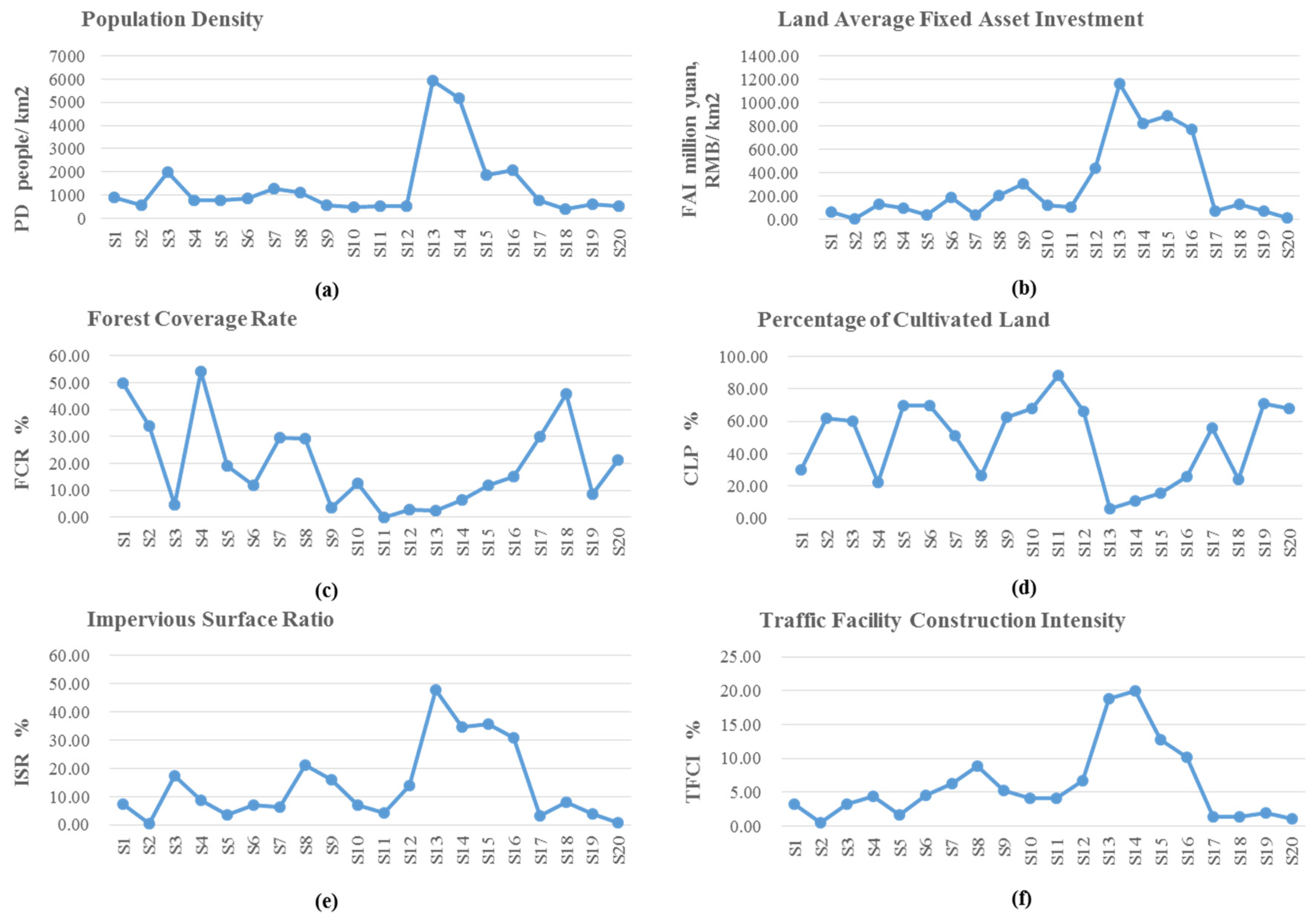
3.1. Descriptive Statistics of Water Quality and LDI Indexes

Table 3 describes the water quality parameter test results of river sampling sites in 20 small watersheds in Liangjiang New Area. It can be seen that the mean concentration of TN, NH3+-N and TP was inferior to the minimum allowable value of Class V water in the “National Surface Water Environmental Quality Standard” (GB3838-2002) [68], and about 70% of the sampling sites exceed the limit value of the Class IV water quality parameters. This shows that the overall water quality of the rivers in the Liangjiang New Area was poor, and the nutrient salt pollution was relatively serious. The nutrient pollution of N and P elements was particularly prominent.
Figure 3 shows the features of six LDI indexes in 20 small watersheds. It can be found that: The forest coverage rate (FCR) value and percentage of cultivated land (CLP) value of 20 watersheds were significantly different. In addition to S13, S14, S15, and S16 (Panxi River, Gailan River, Mao River, and Xiaojia River watersheds), impervious surface ratio (ISR) and traffic facility construction intensity (TFCI) values in different watersheds varied slightly, while population density (PD) and land average fixed asset investment (FAI) values varied much more little by contract. PD, FAI, SP, and TFCI are four indexes reflecting the total amount of urban development and construction, and their values reached the maximum value in the small watersheds where the proportion of construction land were relatively high, such as S13, S14, S15, and S16. Comparatively, the indexes of FCR and CLP, which reflect the amount of non-construction land in the city, were the lowest in those four small watersheds.

3.2. Correlation of LDI Indexes and Water Quality

According to the RDA results, the eigenvalue of the four ordination axes of RDA were 0.338, 0.088, 0.017, and 0.013, respectively, which explained 45.5% of water quality characteristic variance, among which the axis 1 and axis 2 comprehensively explained 93.5% of water quality-LDI indexes information (Table 4). The axis 1 of RDA ordination contains the most information of LDI indexes (Table 5), among which ISR has the largest positive correlation with the axis 1 (r = 0.41). This shows that the axis 1 of each sampling site mainly reflects the gradient changes of ISR.
In order to explore factors of each dimension as independent explanatory variables and common explanatory variables, social and economic factors, construction factors, and environmental factors were taken as main explanatory variables respectively, and factors of the other two dimensions were taken as concomitant variables for partial RDA analysis. According to the independent explanatory variable results of each dimension and the explanatory variable results of the three dimensions obtained in Table 4, the common explanatory part of the three dimensions is obtained by subtraction (Figure 4).

3.2.1. Correlation of Social and Economic Factors and Water Quality

As can be seen from Figure 4, social and economic factors independently explained 43.5% of water quality variance, with the largest independent variance explain in the three dimensions. From the test results of the importance and signification level of individual LDI index in Table 5, the influence of land average fixed asset investment (FAI) on river water quality reached a significant level (p < 0.050), and the amount of the explain for water quality characteristic variance accounted for 30.43% of the total information, which indicates that FAI is an important factor affecting river water quality. The index of population density (PD) did not reach the significant level (p > 0.050), indicating that PD had little effects on water quality in this research.

3.2.2. Correlation of Construction Factors and Water Quality

From Figure 4 that construction factors independently explains 35.4% of water quality variance, with a relatively high explain, which is inferior to social and economic factors’ independent explain in three dimensions. From Table 5, the influence of impervious surface ratio (ISR) on river water quality reached a significant level (p < 0.050), and the amount that could explain the water quality characteristic variance is the highest, accounting for 34.78% of the total information. This indicates that ISR is also one of the key factors affecting the water quality of rivers. The index of traffic facility construction intensity (TFCI) did not reach the significant level (p > 0.050), indicating that TFCI had little effect on water quality in this research.

3.2.3. Correlation of Environmental Factors and Water Quality

As shown in Figure 4, environmental factors accounted for only 14.3% of the variance in water quality independently, with the lowest explanation in the three dimensions. From Table 5, the influence of forest coverage rate (FCR) and percentage of cultivated land (CLP) on river water quality did not reach a significant level (p > 0.050), indicating that FCR and CLP had little effects on water quality in this research. Meanwhile, it is noticed that FCR and CLP were negatively correlated with axial 1 (r = −0.23, −0.24, respectively), showing these two indexes were opposite to the gradient change trend of water quality.

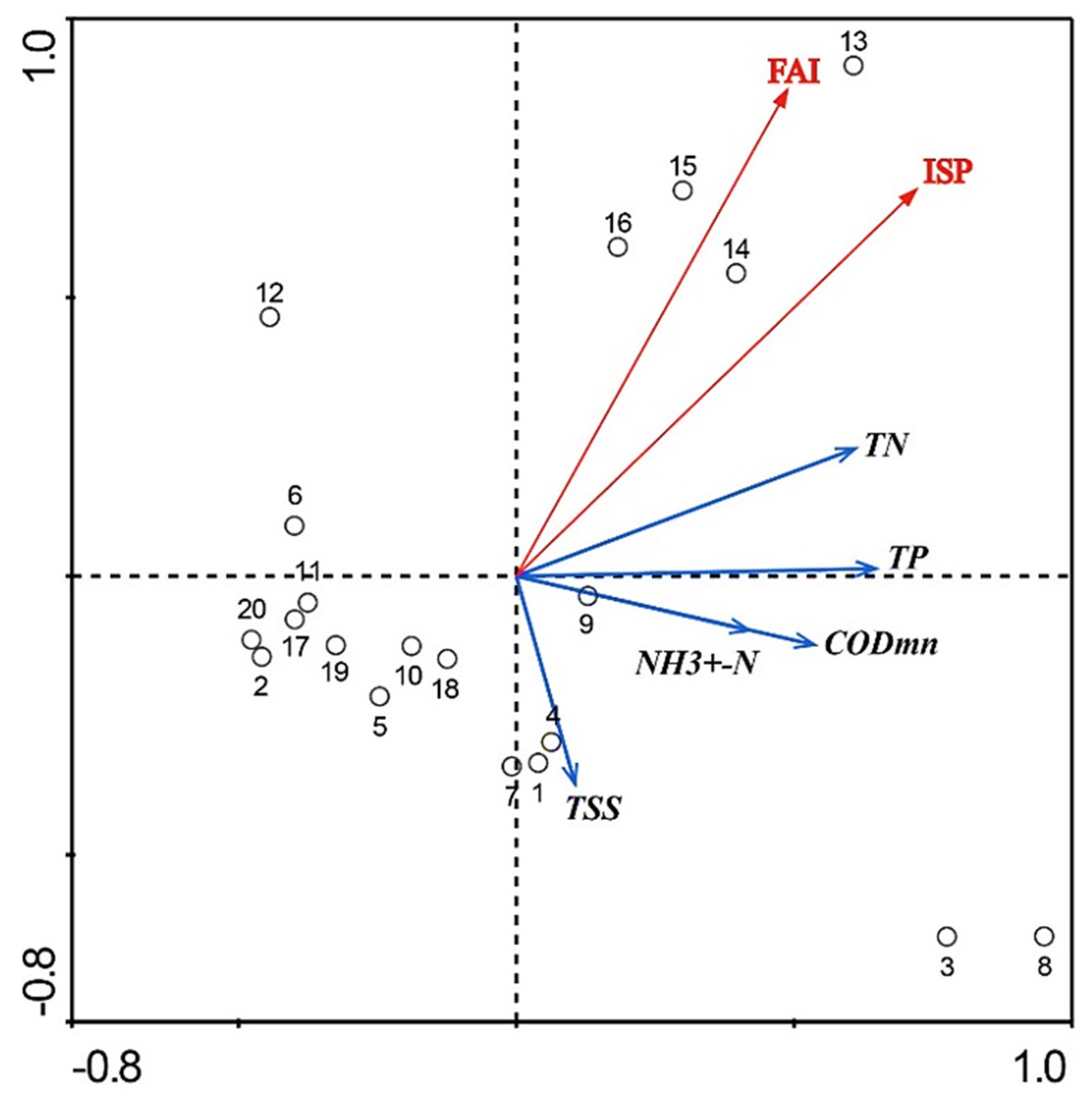
3.3. RDA Ordination Diagram of Indexes with Significant Effects

After the correlation test, the indexes with insignificant effects were screened out, and only the RDA results of the indexes with significant effects were retained. The RDA ordination diagram of impervious surface ratio (ISR) and land average fixed asset investment (FAI) generated from Canoco is shown in Figure 5. The correlation of them are determined by the cosine value of the angle between their axes (Table 6). The positive correlation between LDI indexes and river water quality indicates that this index plays a role in the deterioration of river water quality, and conversely, it plays a role in the purification of river water quality. It can be seen from Figure 5 and Table 6 that ISR and FAI have positive correlations with TN, TP, NH3+-N, and CODMN. The correlation with four water quality parameters is TN > TP NH3+-N = CODMN. The positive correlations of ISR with water quality parameters are all higher than the correlation between FAI and corresponding water quality parameters. ISR and FAI have negative correlations with TSS, and the negative correlation of FAI is higher than that of ISR.

4. Discussion

4.1. Effects of Social and Economic Factors on Water Quality

Land average fixed asset investment (FAI) was proved to be an important index that has a significant impact on river water quality (p = 0.040 *, explain of 30.43%). The size of this index is related to the intensity of human activities on the land, describing the reflection of the total fixed asset investment in industrial and real estate development in the watershed in 2014 in terms of the area of land per unit of the watershed. The total amount of fixed assets investment can accurately describe the economic benefits of the watershed and further reflect the active degree of the local administration of watershed in the investment of landscape development and construction. The larger the investment of fixed assets in industrial land, residential land, and commercial land, the greater the development and construction of the above-mentioned land types, and the higher the possibility of sewage and pollutants. In addition, the index allocates the total amount of fixed asset investment to the land per unit area, which can eliminate the errors caused by the large difference in watershed area to some extent. Interestingly, in this research, ISR and FAI were negatively correlated with TSS. The possible reason for this is that most of the construction land in the city is of smooth, hard, impervious ground, which is cleaned regularly, so there is not too much sediment accumulation.
What is more, it can be observed that in the study area, the FAI of Xiangxi River and Hou River watersheds are similar (204.73 million yuan, RMB/km2 and 192.22 million yuan, RMB/km2, respectively), and the watersheds are in similar positions, both of which are located in the upper reaches of Jialing River. However, the water quality of the watersheds varies greatly: The former had poor water quality with three water quality parameters below the standard, and the latter had better water quality with only TN concentration slightly higher than the minimum allowable value of class V water. It is speculated that this phenomenon may be related to the size of the watersheds: Hou River watershed with better water quality is 28 times larger than Xiangxi River watershed with worse water quality. Similar situations also occurred in Dongliang River and Zhaoyang River watersheds, as well as Zhangjia River and Heishui River watersheds. This proves to a certain extent that FAI has scale effect on water quality, that is, the area of the watersheds with similar FAI and adjacent locations is inversely proportional to the river water quality in the watershed.
Domestic sewage produced by urban population mainly affects river water quality by point source discharge. Although there is a positive correlation between population density (PD) and domestic pollution load [81], most domestic sewage in cities enters sewage treatment plants through interception. According to the local study of Mo et al. [82], there were 5 sewage treatment plants in Liangjiang New Area in 2012, with a sewage treatment rate of 87%. By April 2015, there were 10 sewage treatment plants in operation in Liangjiang New Area, with a total sewage treatment scale of 780,000 tons/day [83], which to a large extent alleviated the pressure of point source pollution on the water environment of the watersheds and greatly reduced the effect of population density on the river water quality. In addition, in urbanized areas, the concentration of population mainly affects water quality by converting land cover into impervious surfaces. However, some areas with higher population density, such as high-rise high-density residential areas, have small effects on water quality because they have less impervious surface area than low-density residential areas [84]. It can be seen that PD in urbanized areas may not have significant correlation with river water quality in this study area.
Social and economic factors have the largest independent explain of water quality variance, which can affect the water environment of a region through capital, technology, decision making, system, and other factors at multiple levels. Urban population aggregation and industrial spatial agglomeration caused by the regulation of social and economic factors have been proved to be the most fundamental cause of water environment degradation [19,85]. Therefore, adjusting social and economic factors on the decision making level is an important way to improve river water quality.

4.2. Effects of Construction Factors on Water Quality

Impervious surface ratio (ISR) was also proved to be a key index with significant influence on river water quality (p = 0.042 *, explain of 34.78%). ISR reflects the proportion of impervious surface area in various plots of construction land within the watershed, including residential land, commercial land, and industrial land. The linear land use for transportation is deducted from the calculation of this index, so the control of land use index is limited to the interior of each plot. As one of the significant features of urbanization and landscape development, the effect of impervious surface on water quality is mainly manifested as increasing non-point source pollution load [86]. The increase of impervious surface area of plot will increase the runoff of rainfall in a short time, and increase the flood frequency and total runoff in a long time. As a whole, the overall impervious surface ratio of watersheds is proportional to the runoff, and plays an important role in urban waterlogging [87].
It is worth noting that in the study area of this research, the ISR of Hou River and Zhangjia River watersheds is similar, and the values are relatively low, which is 6.87% and 6.93%, respectively. However, the area scale of the two watersheds is quite different: The former is 43 times larger than the latter. But in terms of water quality, both watersheds had a relatively good water environment, with only TN concentration slightly higher than the minimum value of class V water. Similarly, the ISR of the Gailan River, Mao River, and Xiaojia River watersheds is close and high (34.75%, 35.81%, and 30.96%, respectively), and the area of the last one is four and five times that of the former two. However, as for the water quality, the concentration of three parameters in all three watersheds was significantly higher than the minimum allowable value of class V water. It can be inferred that: In this research, ISR seems not to show the scale effect on water quality; and at different scales, there is an obvious positive correlation between ISR and river water quality. That is to say, reducing impervious surfaces within a watershed is a suitable adaptation strategy for improving river water quality at any scale [88].
Frequent traffic activity of motor vehicles is an important source of road pollutant accumulation [89]. Rainwater runoff is an important factor affecting water quality in mountainous urban areas with high road slope. Especially in the flood season from June to August, the early rainfall runoff of moderate rainfall and heavy rainfall events has a strong scour effect on pollutants on the roads with high slope, leading to the most obvious runoff pollution [90]. However, the water quality parameters adopted in this research was in April of 2014, which was not the flood season. Therefore, the runoff pollution of the road was not obvious, which may lead to the insignificant correlation between traffic facility construction intensity (TFCI) and water quality in our study.
Construction factors have a relatively large independent explain for water quality variance, and they mainly change the surface runoff and affect the river water quality by changing the land use and land cover, and have the most direct impact on the water environment degradation. Through planning and design strategies, the influence of construction factors on water quality can be effectively controlled.

4.3. Effects of Environmental Factors on Water Quality

Since 2000, Chongqing has responded to and implemented China’s policy of “Grain for green” (returning the cultivated land to forest or pasture). By 2014, the city had completed a total of 12,823.3 km2 of farmland conversion projects assigned by the state [91]. In this process, the possible classification error in land use statistics will lead to the uncertainty of the laws of the effects of forest land and cultivated land on water quality. At the same time, the forest converted from cultivated land in a short period of time may be a “source” rather than a “sink” due to the accumulation of pollutants in the soil, which also makes the effect on water quality uncertain. So in this research forest coverage rate (FCR) and percentage of cultivated land (CLP) were not significantly correlated with water quality parameters, which seems to be inconsistent with the conclusions of relevant studies [30,92,93,94]. In addition, as the water quality parameters collected in this research came from April, which was in the non-flood season, so the non-point source pollutants brought by agricultural activities had not been discharged in a large amount, which led to the result that the correlation between CLP and water quality was not significant. This is consistent with the conclusion of the relevant studies that the effect degree of cultivated land on water quality is seasonal [31,95].
Environmental factors have the least independent explain of water quality variance. The effect of environmental factors such as forest land and cultivated land on water quality mainly depends on the area of the land use and the distance from the water body [30,92,93,94], and the mechanism of environmental factors affecting water quality is relatively single and passive. In addition, relevant studies on the trend of land use change in Liangjiang New Area from 2009 to 2015 showed that the most important transformation direction of land in the study area was the conversion from cultivated land and forest to construction land. The area of cultivated land, forest, garden, villages and water is shrinking year by year, and the reduced land was mainly converted into transportation land and urban land [96]. Therefore, although FCR and CLP had no significant correlation with water quality in this research, given the tradeoff and the game between construction land and non-construction land in rapidly urbanized areas, improving FCR and guaranteeing the area of basic farmland is conductive to playing a role in the river water environment improvement by restraining the further expansion of construction land, most of which are impervious surfaces [30,92].

5. Conclusions

In this research, by selecting indexes that can well evaluate the landscape development intensity in urbanized areas, and exploring the correlation between indexes and river water quality parameters, the indexes that have a great impact on water quality were screened out. The aim of improving water quality of urban rivers then can be achieved by controlling the selected key indexes.
Impervious surface ratio (ISR) describes the scale of development and construction of urban built-up areas from the dimension of construction factors. In the process of rapid urbanization, the higher the impervious surface rate and infrastructure construction intensity are, the worse the water quality is. The control and guidance requirements of ISR are proposed from the planning and design level. On the one hand, control the construction land scale, which means limiting the growth of ISR. Firstly, the growth rate of urban built-up areas should be calculated according to the current scale of construction land based on the development goals of regional social and economic factors, such as the growth rate of population and economy [97], so as to control the immoderate and aimless growth of ISR by limiting the scale. Secondly, on the premise of maintaining the existing construction volume, the ISR can be controlled from the spatial layout of the land. For example, replacing the low-density single-family residential area mode with a high-density community mode, thereby reducing the area of the impervious surface [84].
On the other hand, the river water quality in small watersheds can be improved by reducing the significance of ISR on water quality, which means to reduce the interference of local hydrological circulation feedback effect in small watersheds. For example, under the premise of fixed scale of urban hard ground, one of the planning and design strategy is replacing the impervious ground pavement with permeable concrete and permeable bricks and reduce the significant degree of ISR’s influence on river water quality. Furthermore, the area saved from the compact land layout can be used to increase the natural spaces, which can effectively play the role of runoff interception, such as planning into rainwater gardens, rainwater harvesting tanks and biological pools [98,99,100]. Another sustainable method of runoff disposal is the design and use of infiltration facilities as an integral part of the drainage management of sewerage system of buildings or other paved surfaces, such as infiltration trench, infiltration shaft, and infiltration basin. The basic principle and functions are to divert rainwater to infiltration zone as quickly as possible and to infiltrate into the surrounding soil [99].
Land average fixed asset investment (FAI) describes the intensity of urban landscape development from the dimension of social and economic factors. The assemblage of population, capital, labor, technology, system, and other elements in different regions is one of the important factors that exert great pressure on regional water environment protection [85]. By calculating the threshold range of FAI for deterioration of river water quality, the economic growth rate as well as the amount of asset investment in the watershed can be regulated accordingly. By controlling the size of FAI at the decision making level, the index is within the threshold of deteriorating river water quality, thereby achieving the goal of improving river water quality. What is more, by monitoring the LDI indexes which are highly explanatory and correlated with the variance of river water quality, the future state of river water quality in the study area can be predicted, and the relevant indexes can be timely regulated, so as to deal with the risk and challenge of water quality deterioration in advance.
Furthermore, land use types such as forest, pasture, cultivated land and wetland, as environmental factors, reflect the current situation of the ecological environment of the watersheds, and are also important components of the landscape ecological security pattern of the watershed. They are also the key to maintain the health of the watershed ecosystem and the stability of the regional hydrological cycle. Relevant research shows that forests have a better purification ability to water quality than other environmental factors [31,40,92]. Therefore, the improvement of forest coverage rate (FRC) is also the key to improve river water quality. At the same time, considering the important role of riparian forest as a buffer zone in reducing channel margin erosion, controlling the inputs of fine sediments and nutrients, and protecting the ecological processes in headwater streams [101,102,103], we should first pay attention to the shaping of the natural spaces along the river when increasing the forest coverage rate. What is more, further research can be carried out from the approach of landscape security patterns, and to identify the key parts, points, and location that control water pollution.

Author Contributions

Conceptualization, Y.W. and W.Y.; methodology, W.Y. and J.S.; Software, W.Y.; validation, Y.W., W.Y. and C.C.; formal analysis, J.S.; investigation, W.Y. and J.S.; resources, Y.W. and W.Y.; data curation, W.Y. and J.S.; writing—original draft preparation, J.S. and Y.W.; writing—review and editing, C.C., J.S. and Y.W.; visualization, J.S.; supervision, Y.W., W.Y. and C.C.; project administration, Y.W.; funding acquisition, Y.W.

Funding

The research and activities pertaining to this paper were supported by China National R & D Program “Building strong ecological security patterns through elevating green infrastructure’s level of ecosystem services”, grant number 2017YFC0505705.

Acknowledgments

The authors appreciate so much the Shihu Deng, Chongqing Zhixing Hongtu Technology Co., Ltd. for providing the research data. Also, the authors would like to express their appreciations to the anonymous reviewers and the editors.

Conflicts of Interest

The authors declare no conflict of interest.

References

  1. Viji, J.; Priyanka, J.; Manish, R.; Pawan, L. Assessment of deterioration in water quality from source to household storage in semi-urban settings of developing countries. Environ. Monit. Assess. 2014, 186, 725–734. [Google Scholar] [CrossRef]
  2. Astel, A.; Biziuk, M.; Przyjazny, A.; Namieśnik, J. Chemometrics in monitoring spatial and temporal variations in drinking water quality. Water Res. 2006, 40, 1706–1716. [Google Scholar] [CrossRef] [PubMed]
  3. Tian, Y.; Jiang, Y.; Liu, Q.; Dong, M.; Xu, D.; Liu, Y.; Xu, X. Using a water quality index to assess the water quality of the upper and middle streams of the Luanhe River, northern China. Sci. Total Environ. 2019, 667, 142–151. [Google Scholar] [CrossRef] [PubMed]
  4. Xu, J.; Jin, G.; Tang, H.; Mo, Y.; Wang, Y.-G.; Li, L. Response of water quality to land use and sewage outfalls in different seasons. Sci. Total Environ. 2019, 696, 134014. [Google Scholar] [CrossRef]
  5. Xu, G.; Li, P.; Lu, K.; Tantai, Z.; Zhang, J.; Ren, Z.; Wang, X.; Yu, K.; Shi, P.; Cheng, Y. Seasonal changes in water quality and its main influencing factors in the Dan River basin. Catena 2019, 173, 131–140. [Google Scholar] [CrossRef]
  6. Bahar, M.M.; Ohmori, H.; Yamamuro, M. Relationship between river water quality and land use in a small river basin running through the urbanizing area of Central Japan. Limnology 2008, 9, 19–26. [Google Scholar] [CrossRef]
  7. Rodrigues, V.; Estrany, J.; Ranzini, M.; Cicco, V.D.; Hedo, J.; Lucas-Borja, M.E. Effects of land use and seasonality on stream water quality in a small tropical catchment: The headwater of Córrego Água Limpa, São Paulo (Brazil). Sci. Total Environ. 2017, 622–623, 1553–1561. [Google Scholar] [CrossRef] [Green Version]
  8. Williams, M.R.; King, K.W.; Macrae, M.L.; Ford, W.; Esbroeck, C.V.; Brunke, R.I.; English, M.C.; Schiff, S.L. Uncertainty in nutrient loads from tile-drained landscapes: Effect of sampling frequency, calculation algorithm, and compositing strategy. J. Hydrol. 2015, 530, 306–316. [Google Scholar] [CrossRef]
  9. Margriter, S.C.; Bruland, G.L.; Kudray, G.M.; Lepczyk, C. Using indicators of land-use development intensity to assess the condition of coastal wetlands in Hawaii. Landsc. Ecol. 2014, 29, 517–528. [Google Scholar] [CrossRef]
  10. Haidary, A.; Amiri, B.J.; Adamowski, J.; Fohrer, N.; Nakane, K. Assessing the Impacts of Four Land Use Types on the Water Quality of Wetlands in Japan. Water Resour. Manag. 2013, 27, 2217–2229. [Google Scholar] [CrossRef]
  11. Gu, Q.; Hu, H.; Ma, L.; Sheng, L.; Yang, S.; Zhang, X.; Zhang, M.; Zheng, K.; Chen, L. Characterizing the spatial variations of the relationship between land use and surface water quality using self-organizing map approach. Ecol. Indic. 2019, 102, 633–643. [Google Scholar] [CrossRef]
  12. Meneses, B.M.; Reis, R.; Vale, M.J.; Saraiva, R. Land use and land cover changes in Zêzere watershed (Portugal)—Water quality implications. Sci. Total Environ. 2015, 527–528, 439–447. [Google Scholar] [CrossRef] [PubMed]
  13. Zhao, J.; Lin, L.; Yang, K.; Liu, Q.; Qian, G. Influences of land use on water quality in a reticular river network area: A case study in Shanghai, China. Landsc. Urban Plan. 2015, 137, 20–29. [Google Scholar] [CrossRef]
  14. Giri, S.; Qiu, Z. Understanding the relationship of land uses and water quality in Twenty First Century: A review. J. Environ. Manag. 2016, 173, 41–48. [Google Scholar] [CrossRef] [PubMed] [Green Version]
  15. Muschalla, D. Optimization of integrated urban wastewater systems using multi-objective evolution strategies. Urban Water J. 2008, 5, 59–67. [Google Scholar] [CrossRef]
  16. Shoemaker, C.M.; Ervin, G.N.; DiOrio, E.W. Interplay of water quality and vegetation in restored wetland plant assemblages from an agricultural landscape. Ecol. Eng. 2017, 108, 255–262. [Google Scholar] [CrossRef]
  17. Khare, Y.P.; Martinez, C.J.; Toor, G.S. Water Quality and Land Use Changes in the Alafia and Hillsborough River Watersheds, Florida, USA. JAWRA J. Am. Water Resour. Assoc. 2012, 48, 1276–1293. [Google Scholar] [CrossRef]
  18. Mainali, J.; Chang, H. Landscape and anthropogenic factors affecting spatial patterns of water quality trends in a large river basin, South Korea. J. Hydrol. 2018, 564, 26–40. [Google Scholar] [CrossRef]
  19. Carstens, D.; Amer, R. Spatio-temporal analysis of urban changes and surface water quality. J. Hydrol. 2019, 569, 720–734. [Google Scholar] [CrossRef]
  20. Tang, J.; Li, X.; Cao, C.; Lin, M.; Qiu, Q.; Xu, Y.; Ren, Y. Compositional variety of dissolved organic matter and its correlation with water quality in peri-urban and urban river watersheds. Ecol. Indic. 2019, 104, 459–469. [Google Scholar] [CrossRef]
  21. Shi, B.; Bach, P.M.; Lintern, A.; Zhang, K.; Coleman, R.A.; Metzeling, L.; McCarthy, D.T.; Deletic, A. Understanding spatiotemporal variability of in-stream water quality in urban environments—A case study of Melbourne, Australia. J. Environ. Manag. 2019, 246, 203–213. [Google Scholar] [CrossRef] [PubMed]
  22. Kannel, P.R.; Lee, S.; Lee, Y.-S. Assessment of spatial–temporal patterns of surface and ground water qualities and factors influencing management strategy of groundwater system in an urban river corridor of Nepal. J. Environ. Manag. 2008, 86, 595–604. [Google Scholar] [CrossRef] [PubMed]
  23. Hwang, S.J.; Lee, S.W.; Son, J.Y.; Park, G.A.; Kim, S.J. Moderating effects of the geometry of reservoirs on the relation between urban land use and water quality. Landsc. Urban Plan. 2007, 82, 175–183. [Google Scholar] [CrossRef]
  24. Lee, S.W.; Hwang, S.J.; Lee, S.B.; Hwang, H.S.; Sung, H.C. Landscape ecological approach to the relationships of land use patterns in watersheds to water quality characteristics. Landsc. Urban Plan. 2009, 92, 80–89. [Google Scholar] [CrossRef]
  25. Shen, Z.; Hou, X.; Wen, L.; Aini, G.; Lei, C.; Gong, Y. Impact of landscape pattern at multiple spatial scales on water quality: A case study in a typical urbanised watershed in China. Ecol. Indic. 2015, 48, 417–427. [Google Scholar] [CrossRef]
  26. Paul, M.J.; Meyer, J.L. Streamsin the urban landscape. Annu. Rev. Ecol. Syst. 2001, 32, 333–365. [Google Scholar] [CrossRef]
  27. Tong, S.T.Y.; Chen, W. Modeling the relationship between land use and surface water quality. J. Environ. Manag. 2002, 66, 377–393. [Google Scholar] [CrossRef]
  28. Yu, S.; Xu, Z.; Wei, W.; Zuo, D. Effect of land use types on stream water quality under seasonal variation and topographic characteristics in the Wei River basin, China. Ecol. Indic. 2016, 60, 202–212. [Google Scholar] [CrossRef]
  29. Pratt, B.; Chang, H. Effects of land cover, topography, and built structure on seasonal water quality at multiple spatial scales. J. Hazard. Mater. 2012, 209–210, 48–58. [Google Scholar] [CrossRef]
  30. Ye, L.; Cai, Q.H.; Liu, R.Q.; Cao, M. The influence of topography and land use on water quality of Xiangxi River in Three Gorges Reservoir region. Environ. Geol. 2009, 58, 937–942. [Google Scholar] [CrossRef]
  31. Zhang, J.; Li, S.; Dong, R.; Jiang, C.; Ni, M. Influences of land use metrics at multi-spatial scales on seasonal water quality: A case study of river systems in the Three Gorges Reservoir Area, China. J. Clean. Prod. 2019, 206, 76–85. [Google Scholar] [CrossRef]
  32. Carey, R.O.; Migliaccio, K.W.; Li, Y.; Schaffer, B.; Kiker, G.A.; Brown, M.T. Land use disturbance indicators and water quality variability in the Biscayne Bay Watershed, Florida. Ecol. Indic. 2011, 11, 1093–1104. [Google Scholar] [CrossRef]
  33. Wijesiri, B.; Deilami, K.; Goonetilleke, A. Evaluating the relationship between temporal changes in land use and resulting water quality. Environ. Pollut. 2018, 234, 480–486. [Google Scholar] [CrossRef] [PubMed]
  34. Carroll, S.; Liu, A.; Dawes, L.; Hargreaves, M.; Goonetilleke, A. Role of Land Use and Seasonal Factors in Water Quality Degradations. Water Resour. Manag. 2013, 27, 3433–3440. [Google Scholar] [CrossRef] [Green Version]
  35. Oni, S.K.; Futter, M.N.; Molot, L.A.; Dillon, P.J. Adjacent catchments with similar patterns of land use and climate have markedly different dissolved organic carbon concentration and runoff dynamics. Hydrol. Process. 2014, 28, 1436–1449. [Google Scholar] [CrossRef]
  36. Dillon, P.J.; Kirchner, W.B. The effects of geology and land use on the export of phosphorus from watersheds. Water Res. 1975, 9, 135–148. [Google Scholar] [CrossRef]
  37. Xu, E.; Zhang, H. Aggregating land use quantity and intensity to link water quality in upper catchment of Miyun Reservoir. Ecol. Indic. 2016, 66, 329–339. [Google Scholar] [CrossRef]
  38. Teixeira, Z.; Teixeira, H.; Marques, J.C. Systematic processes of land use/land cover change to identify relevant driving forces: Implications on water quality. Sci. Total Environ. 2014, 470–471, 1320–1335. [Google Scholar] [CrossRef] [Green Version]
  39. Blüthgen, N.; Dormann, C.F.; Prati, D.; Klaus, V.H.; Kleinebecker, T.; Hölzel, N.; Alt, F.; Boch, S.; Gockel, S.; Hemp, A. A quantitative index of land-use intensity in grasslands: Integrating mowing, grazing and fertilization. Basic Appl. Ecol. 2012, 13, 207–220. [Google Scholar] [CrossRef]
  40. Julian, J.P.; Beurs, K.M.D.; Owsley, B.; Davies-Colley, R.J.; Ausseil, A.G.E. River water quality changes in New Zealand over 26 years: Response to land use intensity. Hydrol. Earth Syst. Sci. 2017, 21, 1149–1171. [Google Scholar] [CrossRef] [Green Version]
  41. Zhang, W.; Li, H.; Sun, D.; Zhou, L. A statistical assessment of the impact of agricultural land use intensity on regional surface water quality at multiple scales. Int. J. Environ. Res. Public Health 2012, 9, 4170–4186. [Google Scholar] [CrossRef] [PubMed] [Green Version]
  42. Miserendino, M.L.; Casaux, R.; Archangelsky, M.; Di, P.C.; Brand, C.; Kutschker, A.M. Assessing land-use effects on water quality, in-stream habitat, riparian ecosystems and biodiversity in Patagonian northwest streams. Sci. Total Environ. 2011, 409, 612–624. [Google Scholar] [CrossRef] [PubMed]
  43. Shrestha, S.; Bhatta, B.; Shrestha, M.; Shrestha, P.K. Integrated assessment of the climate and landuse change impact on hydrology and water quality in the Songkhram River Basin, Thailand. Sci. Total Environ. 2018, 643, 1610–1622. [Google Scholar] [CrossRef] [PubMed]
  44. Reiss, K.C.; Hernandez, E.; Brown, M.T. Application of the landscape development intensity (LDI) index in wetland mitigation banking. Ecol. Model. 2014, 271, 83–89. [Google Scholar] [CrossRef]
  45. Brown, M.T.; Vivas, M.B. Landscape development intensity index. Environ. Monit. Assess. 2005, 101, 289. [Google Scholar] [CrossRef]
  46. Lane, C.R.; Brown, M.T.; Murray-Hudson, M.; Vivas, M.B. The Wetland Condition Index (WCI): Biological Indicators of Wetland Condition for Isolated Depressional Herbaceous Wetlands in Florida; Report Submitted to the Florida Department of Environmental Protection (Contract #WM-683); Howard T. Odum Center for Wetlands, University of Florida: Gainesville, FL, USA, 2000. [Google Scholar]
  47. Mark, T.B.; Neal, P.; Alan, F. Spatial Modeling of Landscape Development Intensity and Water Quality in the St. Marks River Watershed; DEP Contract #GW138; Center for Wetlands, University of Florida: Gainesville, FL, USA, 1998. [Google Scholar]
  48. Brown, M.T.; Reiss, K.C. Landscape Development Intensity and Pollutant Emergy/Empower Density Indices as Indicators of Ecosystem Health. In Handbook of Ecological Indicators for Assessment of Ecosystem Health, 2nd ed.; CRC Press: New York, NY, USA, 2010; pp. 171–188. [Google Scholar]
  49. Bonzongo, J.C.J.; Donkor, A.K.; Attibayeba, A.; Gao, J. Linking landscape development intensity within watersheds to methyl-mercury accumulation in river sediments. Ambio 2016, 45, 196–204. [Google Scholar] [CrossRef]
  50. Mack, J.J. Landscape as a predictor of wetland condition: An evaluation of the Landscape Development Index (LDI) with a large reference wetland dataset from Ohio. Environ. Monit. Assess. 2006, 120, 221–241. [Google Scholar] [CrossRef]
  51. Chen, T.S.; Lin, H.J. Development of a framework for landscape assessment of Taiwanese wetlands. Ecol. Indic. 2013, 25, 121–132. [Google Scholar] [CrossRef]
  52. Chen, T.-S.; Lin, H.-J. Application of a Landscape Development Intensity Index for Assessing Wetlands in Taiwan. Wetlands 2011, 31, 745–756. [Google Scholar] [CrossRef]
  53. Liu, M.; Wang, Y.; Dai, Z.; Li, Q. GIS-Based Urban Land Development Intensity Impact Factors Analysis. In Artificial Intelligence and Computational Intelligence; AICI 2012. Lecture Notes in Computer Science, Volume 7530; Lei, J., Wang, F.L., Deng, H., Miao, D., Eds.; Springer: Berlin, Heidelberg, 2012. [Google Scholar]
  54. Hu, Z.-L.; Du, P.-J.; Guo, D.-Z. Analysis of Urban Expansion and Driving Forces in Xuzhou City Based on Remote Sensing. J. China Univ. Min. Technol. 2007, 17, 267–271. [Google Scholar] [CrossRef]
  55. Nina, S.; Matthias, B.; Anna, M.H.; Ewald, K.C. Driving forces and rates of landscape change as a promising combination for landscape change research—An application on the northern fringe of the Swiss Alps. Land Use Policy 2007, 24, 349–361. [Google Scholar] [CrossRef]
  56. Anna, M.H.; Matthias, B. Going beyond landscape change description: Quantifying the importance of driving forces of landscape change in a Central Europe case study. Land Use Policy 2009, 26, 640–648. [Google Scholar] [CrossRef]
  57. Lambin, E.F.; Geist, H.J.; Lepers, E. Dynamics of Land-Use and Land-Cover Change in Tropical Regions. Annu. Rev. Environ. Res. 2003, 28, 205–241. [Google Scholar] [CrossRef] [Green Version]
  58. Tate, C.M.; Cuffney, T.F.; McMahon, G.; Giddings, E.M.P.; Coles, J.F.; Zappia, H. Use of an urban intensity index to assess urban effects on streams in three contrasting environmental settings. Am. Fish. Soc. Symp. 2005, 47, 291–315. Available online: https://www.researchgate.net/publication/228678875 (accessed on 29 September 2019).
  59. Wang, S.; Fang, C.; Wang, Y.; Huang, Y.; Ma, H. Quantifying the relationship between urban development intensity and carbon dioxide emissions using a panel data analysis. Ecol. Indic. 2015, 49, 121–131. [Google Scholar] [CrossRef]
  60. Zhou, D.; Zhang, L.; Hao, L.; Sun, G.; Liu, Y.; Zhu, C. Spatiotemporal trends of urban heat island effect along the urban development intensity gradient in China. Sci. Total Environ. 2016, 544, 617–626. [Google Scholar] [CrossRef]
  61. Zhou, D.; Zhao, S.; Liu, S.; Zhang, L. Spatiotemporal trends of terrestrial vegetation activity along the urban development intensity gradient in China’s 32 major cities. Sci. Total Environ. 2014, 488–489, 136–145. [Google Scholar] [CrossRef]
  62. Wang, S.; Ma, H.; Zhao, Y. Exploring the relationship between urbanization and the eco-environment—A case study of Beijing–Tianjin–Hebei region. Ecol. Indic. 2014, 45, 171–183. [Google Scholar] [CrossRef]
  63. Chuanglin, F.; Jing, W. A Theoretical Analysis of Interactive Coercing Effects Between Urbanization and Eco-environment. Chin. Geogr. Sci. 2013, 23, 147–162. [Google Scholar] [CrossRef]
  64. Wu, J.; Zhong, X.; Peng, J.; Qin, W. Function classification of ecological land in a small area based on ecosystem service bundles: A case study in Liangjiang New Area, China. Acta Ecol. Sin. 2015, 35, 3808–3816. (In Chinese) [Google Scholar]
  65. National Bureau of Statistics. Chongqing Statistical Yearbook—2015; China Statistics Press: Beijing, China, 2015. (In Chinese)
  66. Liao, J. Research on the Response Relationship between River Water Quality and Land-Using in Mountainous City—Taking L-J lake Watershed for Example; Chongqing University: Chongqing, China, 2016; (In Chinese). Available online: http://cdmd.cnki.com.cn/Article/CDMD-10611-1016908149.htm (accessed on 3 October 2019).
  67. Lv, Z.; Qing, X.; Ren, Y.; Wang, X.; Pang, R. Effects of land use pattern on water quality in mountainous city—A case study of Chongqing City. J. Lake Sci. 2016, 28, 319–327. (In Chinese) [Google Scholar] [CrossRef] [Green Version]
  68. State Environmental Protection Administration of China, General Administration of Quality Supervision. Inspection and Quarantine of the PRC. In Water; Chinese Academy of Environmental Sciences, Ed.; China Environmental Science Press: Beijing, China, 2002. (In Chinese) [Google Scholar]
  69. State Environmental Protection Administration of China. Water and Wastewater Monitoring and Analysis Method, 4th ed.; China Environmental Science Press: Beijing, China, 2002. (In Chinese)
  70. Ministry of Land and Resources. (GB/T21010-2017) Current Land Use Condition Classification; China Quality and Standards Publishing & Media Co., Ltd.: Beijing, China, 2017. (In Chinese)
  71. Gong, J.; Chen, W.; Liu, Y.; Wang, J. The intensity change of urban development land: Implications for the city master plan of Guangzhou, China. Land Use Policy 2014, 40, 91–100. [Google Scholar] [CrossRef]
  72. Yao, D.-m.; Chen, Y.-f.; Zhang, F.-g.; Wang, Z.-w.; Zhou, W.-j. Research of the Land Developing Intensity Evaluation of Hainan Province. J. Hebei Agric. Sci. 2008, 12, 86–87. (In Chinese) [Google Scholar] [CrossRef]
  73. National Bureau of Statistics. China Statistical Yearbook—2015; China Statistics Press: Beijing, China, 2015. (In Chinese)
  74. Fu, J.; Jiang, D.; Huang, Y. China Population Grid Distribution Data Set. Acta Geogr. Sin. 2014, 69, 41–44. (In Chinese) [Google Scholar] [CrossRef]
  75. Ping, W.; Wu, W.; Zhu, B.; Wei, Y. Examining the impact factors of energy-related CO2 emissions using the STIRPAT model in Guangdong Province, China. Appl. Energy 2013, 106, 65–71. [Google Scholar] [CrossRef]
  76. Zhao, Y. Research on Change and Modulation of Urban Land Development Intensity in the Yangtze River Delta; Nanjing University: Nanjing, China, 2015. (In Chinese) [Google Scholar]
  77. Qiao, K.; Zhu, W.; Hu, D.; Hao, M.; Chen, S.; Cao, S. Examining the distribution and dynamics of impervious surface in different functional zones of Beijing. Acta Geogr. Sin. 2017, 72, 2018–2031. [Google Scholar] [CrossRef] [Green Version]
  78. Luo, Y.; Zhao, Y.; Yang, K.; Chen, K.; Pan, M.; Zhou, X. Dianchi Lake watershed impervious surface area dynamics and their impact on lake water quality from 1988 to 2017. Environ. Sci. Pollut. Res. 2018, 25, 29643–29653. [Google Scholar] [CrossRef]
  79. Braak, C.J.F.T.; Smilauer, P.J. CANOCO Reference Manual and User’s Guide to Canoco for Windows: Software for Canonical Community Ordination (Version 4.5); Centre for Biometry Wageningen: New York, NY, USA, 2002; pp. 113–180. [Google Scholar]
  80. Lepš, J.Š.P. Multivariate Analysis of Ecological Data Using CANOCO; Cambridge University Press: Cambridge, UK, 2003. [Google Scholar]
  81. Li, Y.; Xu, X.; He, J.; Zheng, Y.; Zhang, K.; Chen, Y.; Li, Z. Point source pollution control and problem in Lake Dianchi basin. J. Lake Sci. 2010, 22, 633–639. (In Chinese) [Google Scholar] [CrossRef]
  82. Mo, D. Study on the Healthy Hydrosocial Cycle—Case of Liangjiang New Area, Chongqing; Chongqing University: Chongqing, China, 2015. (In Chinese) [Google Scholar]
  83. Yan, K. The Building of City Water System Database in Liangjiang New Area of Chongqing Based on the Technology of GIS Chongqing University Chongqing. 2016. (In Chinese). Available online: http://cdmd.cnki.com.cn/Article/CDMD-10611-1016908499.htm (accessed on 7 October 2019).
  84. Stone, B. Paving over paradise: How land use regulations promote residential imperviousness. Landsc. Urban Plan. 2004, 69, 101–113. [Google Scholar] [CrossRef]
  85. Yan, W.; Zhou, Q.; Ye, L. Review of Urdan Land Use Planning and Water Environmental Effects. J. Chongqing Normal Univ. (Nat. Sci.) 2014, 31, 35–41. (In Chinese) [Google Scholar] [CrossRef]
  86. Liu, Z.; Li, Y.; Peng, J. Progress and Perspective of the Research on Hydrological Effects of Urban Impervious Surface on Water Environment. Prog. Geogr. 2011, 30, 275–281. (In Chinese) [Google Scholar] [CrossRef] [Green Version]
  87. Shao, Z.; Fu, H.; Li, D.; Altan, O.; Cheng, T. Remote sensing monitoring of multi-scale watersheds impermeability for urban hydrological evaluation. Remote Sens. Environ. 2019, 232, 111338. [Google Scholar] [CrossRef]
  88. Salerno, F.; Gaetano, V.; Gianni, T. Urbanization and climate change impacts on surface water quality: Enhancing the resilience by reducing impervious surfaces. Water Res. 2018, 144, 491–502. [Google Scholar] [CrossRef] [PubMed]
  89. Kayhanian, M.; Singh, A.; Suverkropp, C.; Borroum, S. Impact of Annual Average Daily Traffic on Highway Runoff Pollutant Concentrations. J. Environ. Eng. 2003, 129, 975–990. [Google Scholar] [CrossRef] [Green Version]
  90. Yan, W.-T.; Han, Y.; He, Q. Characterization of Stormwater Runoff Pollution in Mountain City. J. Civ. Archit. Environ. Eng. 2011, 33, 136–142. (In Chinese) [Google Scholar] [CrossRef]
  91. Guo, Y. Return Farmland to Forest in Chongqing: Bringing Green Water and Green Mountains. (In Chinese). Available online: http://guoqing.china.com.cn/2019-08/21/content_75121622.html (accessed on 23 September 2019).
  92. Sliva, L.; Williams, D.D. Buffer zone versus whole catchment approaches to studying land use impact on river water quality. Water Res. 2001, 35, 3462–3472. [Google Scholar] [CrossRef]
  93. Tang, Z.; Engel, B.A.; Pijanowski, B.C.; Lim, K.J. Forecasting land use change and its environmental impact at a watershed scale. J. Environ. Manag. 2005, 76, 35–45. [Google Scholar] [CrossRef]
  94. White, M.D.; Greer, K.A. The effects of watershed urbanization on the stream hydrology and riparian vegetation of Los Penasquitos Creek, California. Landsc. Urban Plan. 2006, 74, 125–138. [Google Scholar] [CrossRef]
  95. Shi, P.; Zhang, Y.; Li, Z.; Li, P.; Xu, G. Influence of land use and land cover patterns on seasonal water quality at multi-spatial scales. Catena 2017, 151, 182–190. [Google Scholar] [CrossRef]
  96. Fu, J. Study on Land Use Change of Liangjiang New Area in Chongqing. J. Green Sci. Technol. 2017, 180–182. (In Chinese) [Google Scholar] [CrossRef]
  97. Yan, W.; Zhou, J. Ecological Land Use Planning Towards Water Environment Protection at Urban Watershed: Ecological Practice Approaches, Spatial Planning Strategies and Development Transect Models. Urban Plan. Int. 2019, 34, 45–55. (In Chinese) [Google Scholar] [CrossRef]
  98. Wang, Y.; Zhang, H.; Wei, K. Experimental study of permeability in rainwater garden filtration system. J. Southeast Univ. (Nat. Sci. Ed.) 2016, 46, 1308–1312. [Google Scholar] [CrossRef]
  99. Markovič, G.; Zeleňáková, M.; Vranayová, Z.; Kaposztásová, D. Research of Infiltration Facility Efficiency and Quality of Rainwater Harvested from Surface Runoff in Real Conditions; Springer International Publishing: Cham, Switzerland, 2015. [Google Scholar] [CrossRef]
  100. Bakar, A.A.A.; Hassan, N.S. The effectiveness of corn cob activated carbon in rainwater harvesting filtration system. In Proceedings of the International Conference on Technology, Informatics, Management, Engineering & Environment, Bandung, Indonesia, 19–21 August 2014; pp. 86–89. [Google Scholar] [CrossRef]
  101. Tanaka, M.O.; Souza, A.L.T.d.; Moschini, L.E.; Oliveira, A.K.d. Influence of watershed land use and riparian characteristics on biological indicators of stream water quality in southeastern Brazil. Agric. Ecosyst. Environ. 2016, 216, 333–339. [Google Scholar] [CrossRef]
  102. Paula, F.R.d.; Gerhard, P.; Ferraz, S.F.d.B.; Wenger, S.J. Multi-scale assessment of forest cover in an agricultural landscape of Southeastern Brazil: Implications for management and conservation of stream habitat and water quality. Ecol. Indic. 2018, 85, 1181–1191. [Google Scholar] [CrossRef] [Green Version]
  103. Ferreira, A.; Paula, F.R.; Ferraz, S.F.B.; Gerhard, P.; Kashiwaqui, E.A.L.; Cyrino, J.E.P.; Martinelli, L.A. Riparian coverage affects diets of characids in neotropical streams. Ecol. Freshw. Fish 2012, 21, 12–22. [Google Scholar] [CrossRef]
Figure 1. Map of study area.
Sustainability 11 07120 g001
Figure 2. Spatial map of rivers and sampling sites and 20 watershed divisions in Liangjiang New Area of Chongqing.
Sustainability 11 07120 g002
Figure 3. Features of LDI indexes of 20 watersheds: (a) Feature of PD of 20 watersheds, (b) feature of fixed asset investment (FAI) of 20 watersheds, (c) feature of forest coverage rate (FCR) of 20 watersheds, (d) feature of cultivated land (CLP) of 20 watersheds, (e) feature of include impervious surface ratio (ISR) of 20 watersheds, and (f) feature of traffic facility construction intensity (TFCI) of 20 watersheds.
Sustainability 11 07120 g003
Figure 4. The diagram of the independent and common explains of the three dimension factors obtained by partial RDA analysis. The gray part represents the part that water quality variance is jointly explained by the factors of three dimensions, while the white part represents the independent explanation of water quality variance explained by the factors of each dimension.
Sustainability 11 07120 g004
Figure 5. The RDA ordination diagram of impervious surface ratio (ISR) and land average fixed asset investment (FAI). FAI is the amount of fixed asset investment per unit land area of corresponding land use type (million yuan, RMB/km2); ISR is the proportion of impervious surface area of the plot in the watershed area (%).
Sustainability 11 07120 g005
Table 1. Landscape development intensity (LDI) evaluation indexes.
DimensionIndex
LDI IndexesFormulaDescription
Social and economic factors (SEF)Population density (PD) PD = P A i Where, PD is the population per unit land area (people/km2); P is the population in the watershed; i is the number of sampling site within the watershed; A i is the watershed area of the sampling site i .
Land average fixed asset investment (FAI) FAI = ( I k A k I × A i I + R k A k R + A k C × ( A i R + A i C ) ) ÷ A i Where, FAI is the amount of fixed asset investment per unit land area of corresponding land use type (million yuan, RMB/km2); k is the number of the district, and i is the number of sampling site within the watershed; I k is the fixed asset investment of the whole society of industry in the district k ; A k I is the industrial land area of district k ; A i I is the industrial land area of the watershed where sampling site i within district k is located in; R k is the fixed asset investment of the whole society in the real estate development of district k ; A k R is the residential land area of district k ; A k C is the commercial land area of district k ; A i R is the residential land area of the watershed where sampling site i within district k is located in; A i C is the commercial land area of the watershed where sampling site i within district k is located in; A i is the watershed area of the sampling site i .
Construction factors (CF)Impervious surface ratio (ISR) ISR = C i T i A i × ( 1 0.3 ) Where, ISR is the proportion of impervious surface area of the plot in the watershed area (%); i is the number of sampling site within the watershed; C i is the total construction land area in the watershed Where sampling site i is located; T i is the area of transportation land in the watershed where the sampling site i is located; A i is the watershed area of the sampling site i ; 0.3 is the minimum green land rate of the main urban area in the “Technical Provisions of Chongqing Urban Planning Management (2018)”.
Urban traffic facility construction intensity (TFCI) TFCI = T i A i Where, TFCI is the proportion of the area of transportation land in the watershed area (%); i is the number of sampling site within the watershed; T i is the area of transportation land in the watershed where the sampling site i is located; A i is the watershed area of the sampling site i .
Environmental factors (EF) Forest coverage rate (FCR) FCR = F i A i Where, FCR is the proportion of forest area to watershed area (%); i is the number of sampling site within the watershed; F i is the forest area in the watershed where the sampling site is located; A i is the watershed area of the sampling site i .
Percentage of cultivated land (CLP) CLP = P i A i Where: CLP is the percentage of cultivated land in the watershed area (%); i is the number of sampling site within the watershed; P i is the cultivated land area in the watershed where the sampling site i is located; A i is the watershed area of the sampling site i .
Table 2. The lengths of gradient of Detrended Canonical Correspondence Analysis (DCA) of the water quality parameters.
Lengths of Gradient
Axe 1Axe 2 Axe 3Axe 4
1.1050.8460.8230.848
Table 3. Descriptive statistics of water quality parameters of 20 watersheds in Liangjiang New Area of Chongqing. Abbreviations: Total soluble solid (TSS), chemical oxygen demand (CODMN), total nitrogen (TN), ammonia nitrogen (NH3+-N), and total phosphorus (TP).
Water QualityNumber of Sample SitesAverage (mg/L)Minimum
(mg/L)
Maximum
(mg/L)
SDClass IV Standard (mg/L)Class V Standard (mg/L)
TSS2027.49 6.33 114.07 32.45 ≤60≤150
CODMN204.460.57 22.26 4.59 ≤10≤15
TN206.73 1.08 15.63 3.95 ≤1.5≤2
NH3+-N 203.87 0.86 17.62 5.37 ≤1.5≤2
TP200.50 0.04 2.07 0.50 ≤0.3≤0.4
Table 4. Redundancy analysis (RDA) results for LDI indexes and water parameters.
Axis1234Total Inertia
Eigenvalues0.3380.0880.0170.0131.000
Water quality—LDI indexes correlations0.6890.7010.6520.474
Cumulative percentage variance of water quality data33.842.644.245.5
Cumulative percentage variance of water quality—LDI indexes relation74.293.597.1100.0
Sum of all eigenvalues 1.000
Sum of all canonical eigenvalues0.455
Table 5. Importance and signification level of individual LDI indexes and its correlation coefficients of first two RDA axes.
LDI IndexRankImportanceVariance Explains %p-ValueCorrelation with AX1Correlation with AX2
ISR10.1634.78 0.042 *0.410.45
FAI20.1430.43 0.040 *0.260.50
PD30.0613.04 0.2920.370.29
FCR40.048.70 0.434−0.23−0.23
TFCI50.036.52 0.4140.280.50
CLP50.036.52 0.492−0.24−0.35
Note: * Denotes significant relationships at a probability level of <0.05.
Table 6. Correlation matrix of LDI indexes and single river water quality parameters.
LDI IndexesTSSTPTNCODMNNH3+-N
FAI−0.7070.5000.7660.2760.276
ISR−0.4690.7310.9210.5450.545

