Green Activity-Based Costing Production Planning and Scenario Analysis for the Aluminum-Alloy Wheel Industry under Industry 4.0

Abstract

The industrial revolution has grown to the fourth generation, or so-called Industry 4.0. The literature on Industry 4.0 is quite extensive and involves many different dimensions; however, production costs under Industry 4.0 have seldom been discussed. On the other hand, environmental problems are increasingly serious nowadays. Activity-Based Costing is a mature accounting method that can easily trace direct and indirect product costs, based on activities, as well as trace the carbon tax to products, which may lead to different product combinations, in order to reduce environment problems. Thus, the purpose of this paper is to propose a green activity-based costing production planning model under Industry 4.0. In order to make the paper more realistic, we suggest three models with five possible scenarios: normal and material cost fluctuation, material cost discount, and carbon tax with the related cost function. The Aluminum-Alloy Wheel industry was chosen as the illustrative industry to present the results. The model provides managers with a way to deal with the cost problem under Industry 4.0 and to be able to handle the environmental issues in making production decisions. This paper also provides suggestions for governments that have not considered carbon taxation.

1. Introduction

With maturing information, improved communication, and industrial technology, the industrial revolution has grown to the fourth generation, so-called Industry 4.0 [1]. In order to meet the trend, corporations around the world are now facing the huge changes from the traditional factory to the intelligent factory [2]. On the other hand, people around the world are now facing environment problems, such as the ozone hole [3], global warming with its attendant melting arctic ice [4], the emergence of extreme weather [5], etc.; all of these are the result of human destruction of the environment. The green issues have been of concern for many years; governments, corporates, and scholars around the world have also spent much time in exploring different types of green issues.

The current studies on Industry 4.0 have been growing rapidly since the Hannover Fair in Germany (April 2011). The related papers on these issues involve many different dimensions. In engineering, the issues of concern include how to implement, apply or re-engineer [6,7,8,9,10,11,12,13]. In computer science, scholars are not only concerned about the application of the technology of Industry 4.0 [14,15,16], but also the Internet of Things (IoT), Internet of Services (IoS), Cyber-Physical Systems (CPS), and so on. They are also interested in adding various Information Technology (IT) elements to improve communication between humans and machines, as well as data utilization [17,18,19,20,21,22,23,24,25]. In business, management and accounting, the topics include management, control and business strategies [26,27,28,29,30], such as supply chain management, life cycle management, shop floor control, and production control.

The discussions on green issues have continued for more than two decades, from the Kyoto Protocol announced in 1997 to the Paris Agreement announced in 2015, and beyond; the literature also covers various fields. Some of which investigate the relation between society factors and carbon emissions, for example, Begum et al. [31] used econometric approaches to investigate the dynamic impacts on CO2 emissions with GDP growth, energy consumption, and population growth in Malaysia. They found that both per capita energy consumption and per capita GDP has a positive impact with per capita carbon emissions. Friedlingstein et al. [32] and Meinshausen et al. [33] investigated the 2 °C limitation of global warming, they both point out that the current emission of greenhouse gas may exceed the limit and provide a suggestion or a comprehensive probabilistic analysis for further help. There also exist technological ways to reduce the emission quantity of greenhouse gases [34,35].

There are also researchers using mathematical programming to calculate the emission costs in different fields, such as, airlines [36,37], green buildings [38,39,40,41], the electrical and electronic industry [42,43,44], the pulp and paper industry [45], the pharmaceutical industry [46], and the automotive industry [47]. These papers use the Activity-Based Costing method to collect the carbon cost based on activities, they also combine different ways to make the data more realistic, such as stepwise linear function, fuzzy method, and multiple criteria decision making (MCDM).

Both Industry 4.0 and green issue studies have developed to a certain degree; however, cost calculations of green issues under Industry 4.0 have not yet emerged. Moreover, cost issues are always the mainly concern of the entire enterprise, and these concerns differ for each company. Thus, this paper aims to fill this gap by using the Activity Based Costing (ABC) method to collect data, which could increase the accuracy of cost-related data to control the costs of projects [44,48,49,50] after the implementation of Industry 4.0, as well as the taxation of carbon tax on each product to address green issues. This paper also tries to provide different models and possible scenarios to deal with complicated real world business situations, such as material cost fluctuations, price discounts with high quantity purchases, etc.

As illustrated above, this paper selects the Aluminum-Alloy Wheel industry as the example industry, and designs three kinds of models with five possible business scenarios, which include normal, material cost fluctuation, material cost discount, and the carbon tax scenario for further scenario analysis. Considering the cost issues in Industry 4.0, we use labor cost as the linkage. The results show different optimal solutions, based on each scenario. Further explanations for each model and scenario are also proposed.

The remaining sections of this paper are organized, as follows: Section 2 discusses the research background; the literature on Industry 4.0, the green production approach, and environmental protection in the Aluminum-Alloy Wheel industry will be introduced. Section 3 presents a green production-planning model under ABC and Industry 4.0; in this section, the cost of each activity can be calculated, as based on the proposed model and assumed scenarios. Section 4 deals with the example data, which show the results based on Section 3. A brief discussion and conclusions are given in Section 5.

2. Literature Review

2.1. Brief Introduction to Industry 4.0

The term “Industry 4.0” was revealed for the first time at the Hannover Fair in April 2011 [1]. According to the dream car report [51], the origin of this term can be traced back to the vision of the industry of the future by the Communication Promoters Group of the Industry Science Research Alliance. With the promotion of this group, the federal government adopted the project “Industry 4.0” in November 2011 as part of its High-Tech Strategy action plan. At the same time, the Communication Promoters Group initiated the Working Group Industry 4.0, and the first implementation recommendations on Industry 4.0 were developed from January to October 2012; they also accomplished the final report, which included eight fields of action, and proposed it to German Chancellor Angela Merkel at the Hannover Fair in 2013.

The term “Industry 4.0” is a collective concept which contains technologies and concepts of value chain organization [9], such as CPS, IoT, IoS, Smart Factory, and so on. With CPS, the real world and virtual world can be connected together, for example, the refrigerator, washing machine, or other physical objects with a sensor, storage or other intelligent components can deliver the data through the internet to communicate with each other. CPS is also a key factor as a technological enabler of Industry 4.0 [51]. With IoT, objects with internet components, such as Wi-Fi devices, can be easily connected together [52]. The IoT is also a key component in Industry 4.0; it not only can help CPS communicate with each other, but also provide information to humans in real time [9].

The cost issues related to Industry 4.0 already exist in the literature. Ślusarczyk [53] offered an overview on Industry 4.0 and illustrated the expected level of cost reduction, which included weighted average with 3.6% decrease, transportation and logistics with 3.2% decrease, metals with 3.2% decrease, industrial manufacturing with 3.6% decrease, forest, paper, and packaging with 4.2% decrease, engineering and construction with 3.4% decrease, electronics with 3.7% decrease, automotive with 3.9% decrease, and aerospace, defense, and security with 3.7% decrease. Lee et al. [54] illustrated the trends of manufacturing service transformation in big data environments. The author made some conclusions and mentioned that “labor costs will reduce due to the new trend of industry” and “costs will be reduced by energy-saving, optimized maintenance scheduling, and supply chain management”.

2.2. Industry 4.0 and Aluminum-Alloy Wheel Industry

Although literature regarding the impact of the introduction of Industry 4.0 on the aluminum-alloy wheel industry is scarce, current application has already been shown in exhibitions around the world. In the 2018 Taipei Intelligent Machinery & Manufacturing Technology Show (iMTduo), the Aluminum-Alloy Wheel industry first presented their applications of Industry 4.0. These applications included Automatic Virtual Metrology (AVM), Augmented and Virtual Reality (AVR), and Intelligent Predictive Maintenance (IPM). With AVM, real time data is sent to the cloud, where anyone can monitor the production process in real time; it also can reduce waste and defect loss during the production process. With AVR and IPM, engineers can obtain the current status and remaining life of each machine part, as well as the ability to conduct remote maintenance.

2.3. Green Production and Environmental Protection in the Aluminum-Alloy Wheel Industry

Green issues have led to many entities trying to reduce carbon emissions. In the aluminum-alloy industry, reducing the material weight is a popular method; for example, Yilmaz et al. [55] used three kinds of aluminum alloy to reduce the weight of vehicle doors. Other scholars also employed a lightweight approach to reduce fuel consumption in order to reduce emission quantities [56,57,58,59]. Another relevant way, but still related to weight, employed by the aluminum alloy wheel industry involves structural changes or using different casting methods. Deschamps et al. [60] examined the interplay between improving the alloys and the part’s geometry in seeking to reduce the weight; Peng et al. [61] added other materials in the casting process to reduce the weight.

3. Green Production Planning Model under ABC and Industry 4.0

3.1. A Production Process for a Typical Aluminum-Alloy Wheel Company

The traditional aluminum alloy wheel companies’ production process is simplified, as shown in Figure 1. In this figure, the oval signifies the input/output of an aluminum alloy wheel, where the input will be aluminum ingot or aluminum alloy and the output will be saleable products; the square means the production process of the aluminum alloy wheel. The overall process can be divided into four parts: Casting, Heat Treatment, Computer Numerical Control (CNC) Processing, and Painting. The CNC Processing can be broken down into first time and second time processing, the use of second time processing will depend on different product types. For example, the typical car wheel may only need the first time CNC process, but the customized vehicle wheel may need both the first time and second time of CNC processing.

This section is divided into subheadings, which provide concise and precise descriptions of the experimental results, as well as their interpretations and the experimental conclusions that can be drawn.

3.2. Assumptions

In this paper, as assumed, the example of company’s profit comes from three types of green products: Car rims (i = 1), Truck rims (i = 2), and Customized car rims (i = 3). In order to be more realistic, this paper proposes three models with five different business scenarios. Where Model A includes the normal scenario and the material fluctuation scenario, which includes rising and falling material costs; Model B is a material discount scenario; and Model C is an environment scenario. Other assumptions used in this green production-planning model are listed below:

• All activities in this green ABC model are divided into unit-level and batch-level.
• The related resources driven and activity driver have been chosen by the example company.
• The unit-selling prices of all products remain the same in the relevant period.
• The material cost remains the same in the relevant period during the normal and fluctuation scenarios, but when the total purchasing material quantity exceeds that of the first segment, the purchase receives a 1.4% discount for all material, and a 4.2% discount for all material when the purchase quantity exceeds that of the second segment.
• The direct labor hours according to government policy can be extended by using first overtime work and second overtime work.
• The carbon tax is taxed at different rates of different emission quantities.
• The direct labor resources and machine hour resources cannot use outsourcing to expand.

The remainder of this section is, as follows. In Section 3.3, Model A, the ABC model without other business scenarios is introduced. It includes objective function, unit-level labor cost function, batch-level activity cost function, and other sales and production constraints. In Section 3.4, Model B, the material discount scenario is introduced. The objective function and other functions and constraints are based on the Model A mentioned in Section 3.3; a discount function and constraint are added in this scenario. Lastly, Model C considers the carbon tax scenario. The objective function and another constraint are based on Model B, as mentioned in Section 3.4, and the added carbon tax function and constraint are illustrated in Section 3.5.

3.3. Model A: ABC Model without Other Business Scenarios

Model A considers the basic business situation, and contains the objective function with Equation (1_A), the constraints of unit-level direct labor cost function with Equations (2) to (7), the constraints of batch-level activity cost functions for material handling and setup activities with Equations (8) to (11), and other sale and production constraints with Equation (12) and Equation (13). The following subsection introduces the objective function in detail, as well as the associated constraints.

3.3.1. Objective Function

The objective function of the green production-planning model under ABC and Industry 4.0 is as follows:

The company’s maximized profit π = the sales revenue of each product − total direct material consumption cost − labor hour cost − unit-level activity cost − batch-level activity cost − carbon tax − other fixed cost

$$\begin{gathered} \mathsf{\pi }={\displaystyle \sum }_{\mathrm{i}=1}^{\mathrm{n}}{P}_i{X}_i-{\displaystyle \sum }_{\mathrm{i}=1}^{\mathrm{n}}{\displaystyle \sum }_{\mathrm{k}=1}^2{C}_k{q}_{ik}{X}_i-[{LC}_1+{\sigma }_1({LC}_2-{LC}_1)+{\sigma }_2({LC}_3-{LC}_1)] \\ {-d}_j{\eta }_j{B}_j-{\displaystyle \sum }_{\mathrm{i}=\mathrm{1}}^n{d}_j{\gamma }_{ij}{B}_{ij}-F \end{gathered}$$

(1_A)

where

π	The company’s profit
Pi	Unit prices when selling one unit of product i
Xi	Total produced quantity of product i
Ck	Costs of material k when each unit consumed
qik	The consumption quantity of material k when producing one unit of product i
LC1, LC2, LC3	Total direct labor cost for normal labor hours (LC1), first overtime (LC2) and second overtime (LC3) work
σ0, σ1, σ2	A special ordered set of type 2 (SOS2) variable, which must be a set of positive variables; at most two variables in ordering can be non-zero [62]
dj	The activity cost when executing one unit of activity j
ηj	The batch-level activity (j ∈ B) driven requirement for material handling activity
γij	The batch-level activity (j ∈ B) driven requirement for product i at a setup activity
Bj	The quantity of batch-level activity (j ∈ B) at material handling activity
Bij	The quantity of batch-level activity (j ∈ B) for product i at setup activity
F	The company’s reaming fixed costs

The detailed description of the above model will be introduced in the subsection below; however, the direct material cost is simpler than the others so we included it here instead of in an independent subsection. The term ${{\displaystyle \sum }}_{i=1}^n{{\displaystyle \sum }}_{k=1}^2{C}_k{q}_{ik}{X}_i$ in the second set of Equation (1_A) represents total direct material cost. Based on the assumption proposed in Section 3.2, this model’s material cost under normal scenario will be the fixed direct material costs at any quantity. Other cost functions and constraints: the detailed description of other functions and constraints, such as labor cost function, batch-level activity function, etc., are described in the following sections.

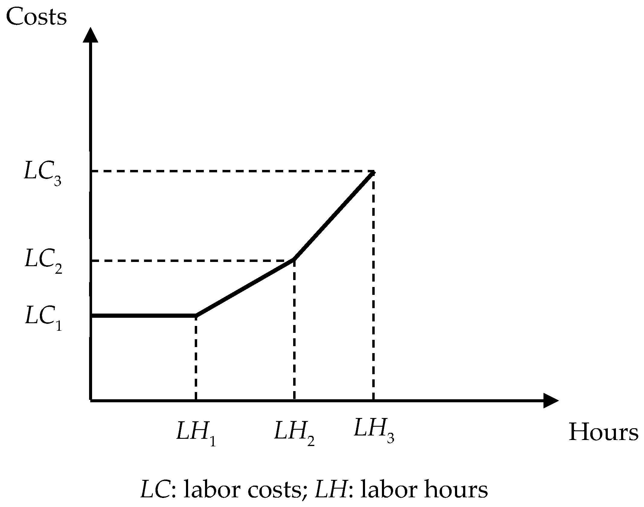
3.3.2. Unit-Level Direct Labor Cost Function

The term $\left[L{C}_1+{\sigma }_1\left(L{C}_2-L{C}_1\right)+{\sigma }_2\left(L{C}_3-L{C}_1\right)\right]$ in the third set Equation (1_A) represents the unit-level direct labor cost. Equations (2) to (7) represent the constraints of the direct labor resources. The direct labor resources and their costs are separated into normal, first overtime, and second overtime work hours. The relevant work hours and wage rates can be composed into three segments of piecewise linear function, as shown in Figure 2. In Equations (2) to (7), (β₁, β₂) is a special ordered set of type 1 (SOS1) variable, so, when one of the variables is set to one, another variable must be exactly zero; (σ₀, σ₁, σ₂) is an SOS2 variable, which must be a set of positive variables; at most, two variables in the ordering can be non-zero [62]. If β₁ = 1, then β₂ = 0 (Equation (7)), σ₀, σ₁ ≤ 1 (Equations (3), (4)), σ₂ = 0 (Equation (5)), and σ₀ + σ₁ = 1 (Equation (6)). This means the direct labor hours and cost are σ₀LH₁ + σ₁LH₂ and σ₀LC₁ + σ₁LC₂, respectively. It also means that the point (σ₀LH₁ + σ₁LH₂, σ₀LC₁ + σ₁LC₂) is located at the second part of the unit-level direct labor cost function with the first overtime work; this point is also a combination of (LH₁, LC₁) and (LH₂, LC₂). On the other hand, if β₂ = 1, then β₁ = 0 (Equation (7)), σ₁, σ₂ ≤ 1 (Equations (4),(5)), σ₀ = 0 (Equation (3)), and σ₁ + σ₂ = 1 (Equation (6)). This means the direct labor hours and cost are σ₁LH₂ + σ₂LH₃ and σ₁LC₂ + σ₂LC₃, respectively. It also means that the point (σ₁LH₂ + σ₂LH₃, σ₁LC₂ + σ₂LC₃) is located at the third part of the unit-level direct labor cost function with the second overtime work, and this point is also a combination of (LH₂, LC₂) and (LH₃, LC₃). The first segment of the unit-level direct labor cost function was set to a fixed cost, which means: (1) no matter how many labor hours were used, the cost remains the same; and (2) no matter whether β₁ = 1 or β₂ = 1, the cost will always be added.

Constraints

$${\displaystyle \sum }_{\mathrm{i}=1}^{\mathrm{n}}(l_{i1}+l_{i2}+l_{i3}+{\theta }_i{l}_{i4}+l_{i5})X_i\le {LH}_1+{\sigma }_1({LH}_2-{LH}_1)+{\sigma }_2(L{H}_3-{LH}_1)$$

(2)

$${\sigma }_0-{\beta }_1\le 0$$

(3)

$${\sigma }_1-{\beta }_1-{\beta }_2\le 0$$

(4)

$${\sigma }_2-{\beta }_2\le 0$$

(5)

$${\sigma }_0+{\sigma }_1+{\sigma }_2=1$$

(6)

$${\beta }_1+{\beta }_2=1$$

(7)

where

li1, li2, li3, li5	The usage of labor hours at the first to third and fifth activity when producing one unit of product i
θili4	The usage of labor hours at the fourth activity when producing one unit of product i, and multiplying a coefficient use to determine how much work should be done in the fourth activity
LH1, LH2, LH3	Maximum capacity of direct labor hours at normal (LH1), first overtime (LH2) and second overtime (LH3) work hours
β1, β2	An SOS1 variable, when one of the variables is set to one, another variable must be exactly zero [62].

3.3.3. Batch-Level Activity Cost Function for Material Handling and Setup Activities

The terms $d_j{\eta }_j{B}_j$ and ${{\displaystyle \sum }}_{i=1}^n{d}_j{\gamma }_{ij}{B}_{ij}$ in the fourth and fifth set of Equation (1_A) represent batch-level activity cost functions for material handling and setup activities. Equations (8) and (9) are the constraints of material handling, and Equation (10) and (11) are the constraints of setup activities. We assumed that the material handling stage only considers the procedure from raw material storage location to factory, but the setup activities were considered at each activity. For example, the setup hours are used to measure the setup activity, where T_j represents the setup hours that can be used, γ_ij represents the setup hours needed for j activity for product i; M_ij represents i product’s setup unit in each setup batch.

$${\displaystyle \sum }_{\mathrm{i}=1}^{\mathrm{n}}{q}_{i1}{X}_i\le {\varnothing }_j{B}_j (j=6)$$

(8)

$${\eta }_j{B}_j\le T_j (j=6)$$

(9)

where

∅j	The quantity per batch of batch-level activity (j ∈ B) at material handling activity
Tj	The capacity of batch-level activity (j ∈ B)

$$X_i\le M_{ij}{B}_{ij} (j=7,i=1\dots 3)$$

(10)

$${\displaystyle \sum }_{i=1}^n{\gamma }_{ij}{B}_{ij}\le T_j (j=7)$$

(11)

where

Mij	The quantity per batch of batch-level activity (j ∈ B) for product i at setup activity

3.3.4. Other Sale and Production Constraints

The constraints in this part do not influence the profit directly, but will indirectly influence the profit because of the limitation of the resources. Equations (12) and (13) represent the machine hour constraints for activities 1, 2, and 5 and for activities 3 and 4 so-called CNC, respectively. In Equation (12), when the factory produces one unit of product i, it will need h_i hours at activity j. Each activity has its own capacity MH_j. In Equation (13), when the factory produces one unit of product i, it will need h_i3 hours and additional reprocessing hours with coefficient θ_ih_i4 at activity CNC; Activity 3 and 4 shared the capacity MH_CNC.

$${\displaystyle \sum }_{\mathrm{i}=1}^{\mathrm{n}}{h}_{ij}{X}_i\le {MH}_j (j=1,2,5)$$

(12)

$${\displaystyle \sum }_{\mathrm{i}=1}^{\mathrm{n}}\left(h_{i3}{X}_i+{\theta }_i{h}_{i4}\right)\le {MH}_{CNC}$$

(13)

where

hij	The requirement hours when producing a single unit of product i at activity j
MHj	The total available machine hours of activity j
hi3	The requirement hours when producing a single unit of product i at the third activity
θihi4	The requirement hours when producing a single unit of product i at the fourth activity, and multiplying a coefficient use to determine how much work should be done in the fourth activity
MHCNC	The total capacity of machine hours of the third and fourth activities

3.4. Model B: ABC Model with Material Discount

Model B considers material discount from the basic business situation of Model A. Model B includes the objective function with Equation (1_B), which was changed based on Model A. The related constraints associated with material discount are Equations (14) to (18). The constraints associated with other cost functions from Equations (2) to (13) remain the same. That is, Model B includes the objective function with Equation (1_B) and the related constraints with Equations (2) to (18). The following subsection introduces the objective function and material discount function in detail.

3.4.1. Objective Function

In this subsection, the material discount business scenario is considered and the objective function which was changed based on Equation (1_A), is also proposed. In Model B, assume that only the first material has the material quantity discount.

$$\begin{gathered} \mathsf{\pi }={\displaystyle \sum }_{i=1}^n{P}_i{X}_i-({DC}_1{Q}_1+{DC}_2{Q}_2+{DC}_3{Q}_3+{\displaystyle \sum }_{i=1}^n{C}_2{q}_{i2}{X}_i) \\ -[{LC}_1+{\sigma }_1\left({LC}_2-{LC}_1\right)+{\sigma }_2\left({LC}_3-{LC}_1\right)]-d_j{\eta }_j{B}_j-{\displaystyle \sum }_{i=1}^n{d}_j{\gamma }_{ij}{B}_{ij}-F \end{gathered}$$

(1_B)

where

C2	Unit costs of the second material
qi2	The consumption quantity of the second material when producing a single unit of product i
DC1, DC2, DC3	Unit costs of the first material at normal (DC1), first (DC2) and second (DC3) discount situations
Q1, Q2, Q3	The consumption quantity of first material at normal (Q1), first (Q2) and second (Q3) discount situations

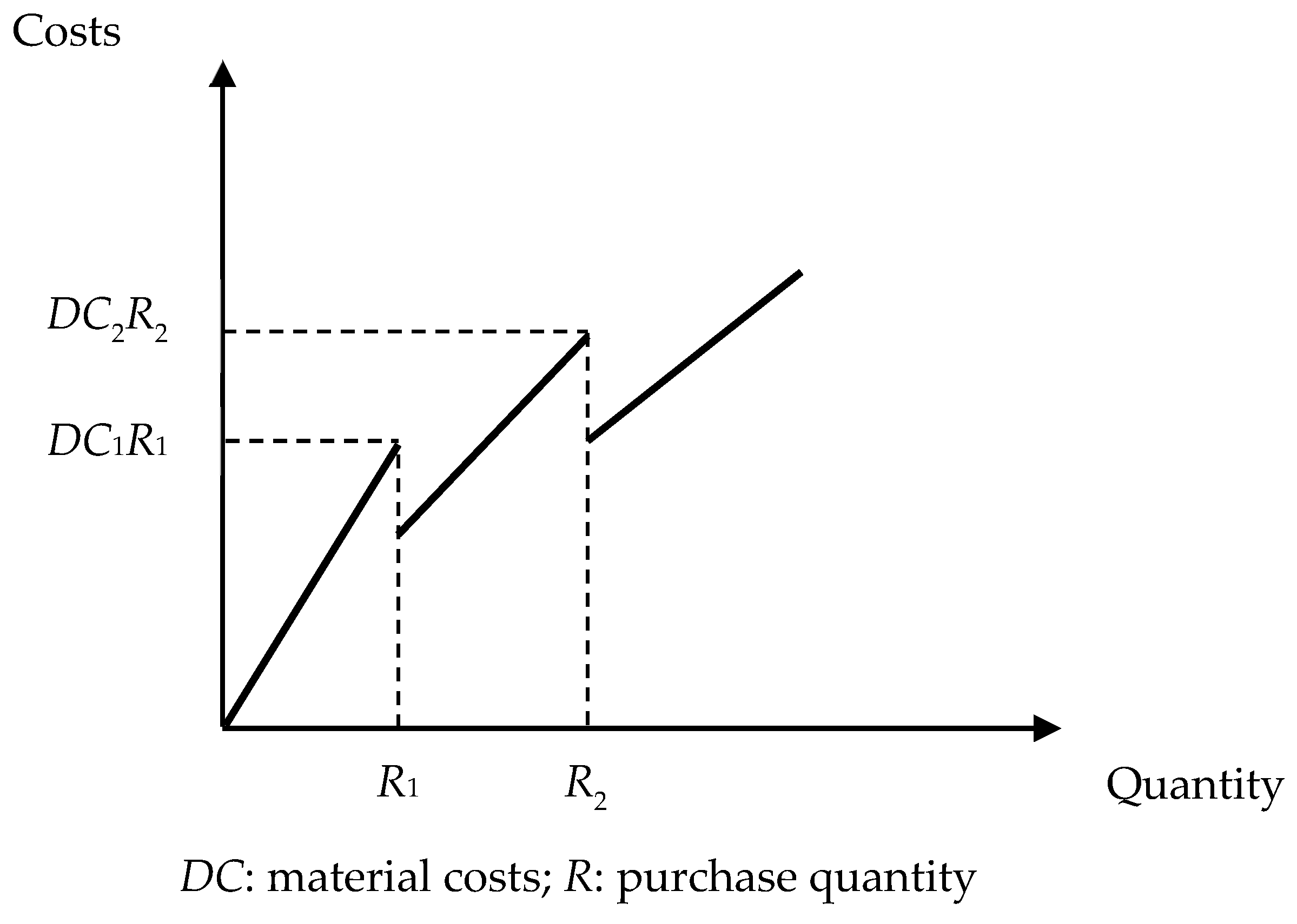
3.4.2. Material Discount Function

The material discount is a very common business scenario in the real world. This study uses three segments of piecewise linear function, as shown in Figure 3. In Equations (14) to (18), (φ₀, φ₁, φ₂) is an SOS1 variable; when one of the variables is set to one, another variable must be exactly zero. If φ₁ = 1, then φ₂, φ₃ = 0 (Equation (18)), Q₂, Q₃ = 0 (Equations (15) and (17)), Q₁ ≥ 0, Q₁ ≤ φ₁R₁ (Equation (16)). This means that the material quantity and cost are Q₁ and DC₁Q₁, respectively, and are on the first segment of the material cost function. On the other hand, if φ₂ = 1, then φ₁, φ₃ = 0 (Equation (18)), Q₁, Q₃ = 0 (Equations (16) and (17)), Q₂ ≥ φ₂R₁, Q₂ ≤ φ₂R₂ (Equation (15)). This means that the material quantity and cost are Q₂ and DC₂Q₂, respectively, and are on the second segment of the material cost function. The third segment of the material cost function does not set the bundle, which means the quantity more than R₂ will be at the same cost DC₃Q₃.

Constraints

$${\displaystyle \sum }_{\mathrm{i}=1}^{\mathrm{n}}{q}_{i1}{X}_i=Q_1+Q_2+Q_3$$

(14)

$$0\le Q_1\le {\phi }_1{R}_1$$

(15)

$${\phi }_2{R}_1<Q_2\le {\phi }_2{R}_2$$

(16)

$${\phi }_3{R}_2<Q_3$$

(17)

$${\phi }_1+{\phi }_2+{\phi }_3=1$$

(18)

where

R1, R2	Maximum purchase quantity of material at normal (R1) and first discount (R2) situation
φ1, φ2, φ3	An SOS1 variable; when one of the variables is set to one, another variable must be exactly zero [62].

3.5. Model C: ABC Model with Material Discount and Carbon Tax

Model C considers carbon tax with a material discount and the basic business situation. Model C contains the objective function with Equation (1_C), which was changed based on Model B. The related constraints with the carbon tax function are Equations (19) to (24). Other cost functions from Equation (2) to Equation (18) remain the same. That is, Model C includes the objective function with Equation (1_C) and the related constraints with Equation (2) to (24). The following subsection introduces the objective function and carbon tax function in detail.

3.5.1. Objective Function

In this subsection, the material discount and carbon tax business scenario is considered, and the objective function which was changed based on Equation (1_B), is also proposed.

$$\begin{gathered} \mathsf{\pi }={\displaystyle \sum }_{i=1}^n{P}_i{X}_i-({DC}_1{Q}_1+{DC}_2{Q}_2+{DC}_3{Q}_3+{\displaystyle \sum }_{i=1}^n{C}_2{q}_{i2}{X}_i) \\ -\left[{LC}_1+{\sigma }_1\left({LC}_2-{LC}_1\right)+{\sigma }_2\left({LC}_3-{LC}_1\right)\right]-d_j{\eta }_j{B}_j-{\displaystyle \sum }_{i=1}^n{d}_j{\gamma }_{ij}{B}_{ij} \\ -({\delta }_1{CCE}_1+{\delta }_2{CCE}_2)-F \end{gathered}$$

(1_C)

where

CCE1, CCE2	The CO2 emission cost at the first extended (CCE1) situation and second extended (CCE2) situation
δ0, δ1, δ2	An SOS2 variable, which must be a set of positive variables; at most two variables in the ordering can be non-zero [62]

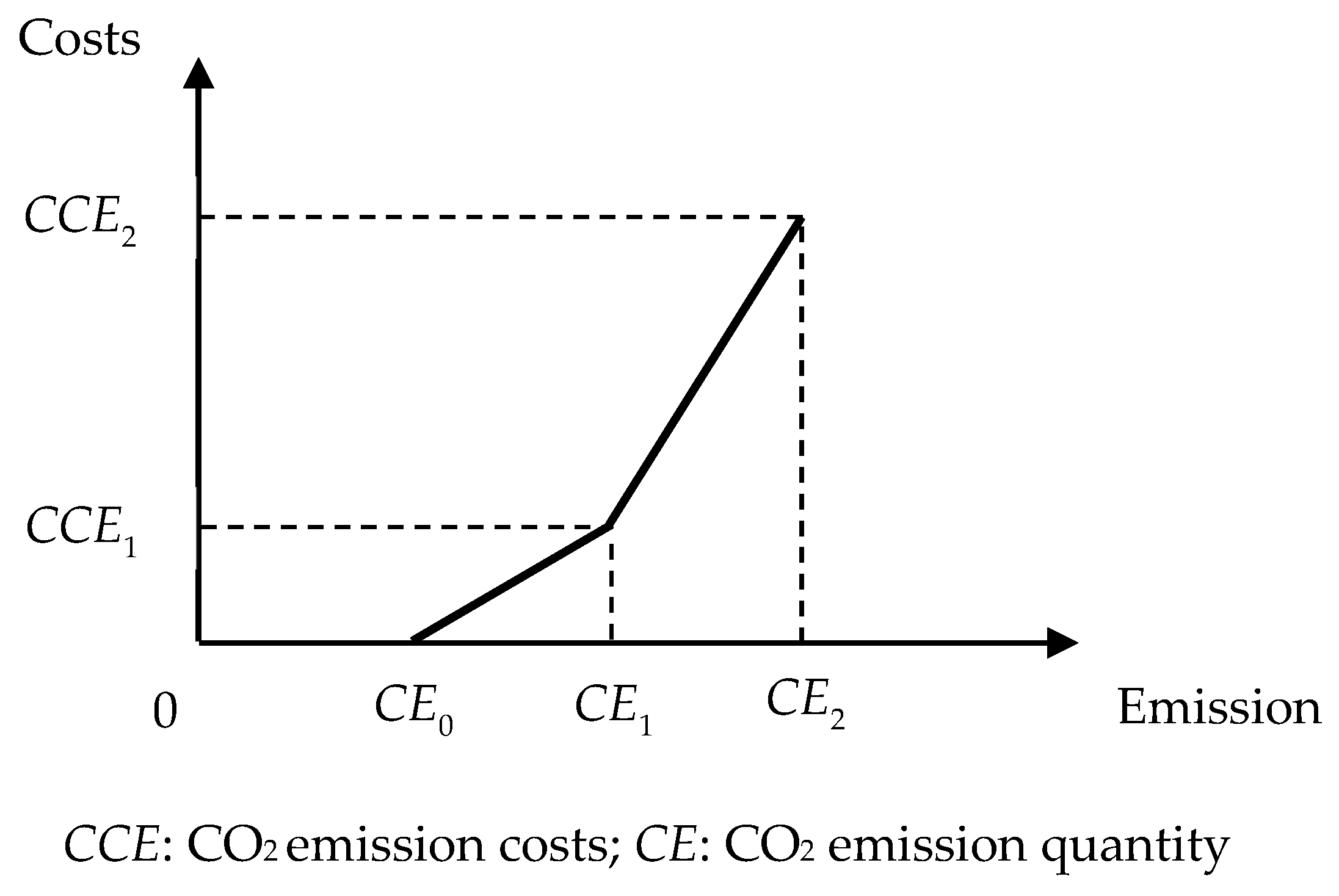
3.5.2. Carbon Tax Function

The carbon tax is considered in this paper. This study also uses three segments of piecewise linear function shown in Figure 4. In Equations (19) to (24), (λ₁, λ₂) is an SOS1 variable; when one of the variables is set to one, another variable must be exactly zero. If λ₁ = 1, then λ₂ = 0 (Equation (24)), δ₀, δ₁ ≤ 1 (Equations (20), (21)), δ₂ = 0 (Equation (22)), and δ₀ + δ₁ = 1 (Equation (23)). This means that the emission quantity and cost are δ₁CE₁ and δ₁CCE₁, respectively. It also means that the point (δ₁CE₁, δ₁CCE₁) is on the second segment of the carbon tax function. On the other hand, if λ₂ = 1, then λ₁ = 0 (Equation (24)), δ₁, δ₂ ≤ 1 (Equations (21), (22)), δ₀ =0 (Equation (20)), and δ₁ + δ₂ = 1 (Equation (23)). This means that the emission quantity and cost are δ₁CE₁ + δ₂CE₂ and δ₁CCE₁ + δ₂CCE₂, respectively. It also means that the point (δ₁CE₁ + δ₂CE₂, δ₁CCE₁ + δ₂CCE₂) is on the of carbon tax function. The first segment of the carbon tax function was set to a free cost, which means: (1) no matter how much carbon was emitted, the cost remains the same; and (2) no matter λ₁ = 1 or λ₂ = 1, the cost will always be free.

Constraints

$${\displaystyle \sum }_{\mathrm{i}=1}^{\mathrm{n}}{e}_i{X}_i\le {CE}_0+{\delta }_1({CE}_1-{CE}_0)+{\delta }_2({CE}_2-{CE}_0)$$

(19)

$${\delta }_0-{\lambda }_1\le 0$$

(20)

$${\delta }_1-{\lambda }_1-{\lambda }_2\le 0$$

(21)

$${\delta }_2-{\lambda }_2\le 0$$

(22)

$${\delta }_0+{\delta }_1+{\delta }_2=1$$

(23)

$${\lambda }_1+{\lambda }_2=1$$

(24)

where

ei	The CO2 emission quantity when producing one unit of product i
CE0, CE1, CE2	The CO2 emission quantity at normal (CE0), first extended (CCE1) situation and second extended (CCE2) situation
λ1, λ2	An SOS1 variable; when one of the variable is set to one, another variable must be exactly zero [62]

4. Illustration

In this section, a numerical example is proposed to find the optimal production combination in each model proposed. Company L was chosen as our example company, as an international company that not only sells basic aluminum alloy wheels, but also customized ones.

Following the global trend, Company L decided to implement Industry 4.0; however, this entails changing the production line process and entailing costs. Thus, this paper presents mathematical decision models to help Company L find the best product combination based on Industry 4.0 under an ABC model. LINGO is the best software to solve such complex mathematical decision models.

4.1. Example Data and Optimal Decision Analysis

Company L mainly produces three kinds of products: Car Rims, Truck Rims, and customized Car Rims. Due to the basic product, car rims and truck rims are set with the minimal requirements. Each product consumes two kinds of material: aluminum ingots (m = 1) and pigment (m = 2), where aluminum ingots encounter material discounts and material fluctuation. Each product requires eight kinds of primary activity, six for the unit-level activity, and two for the batch-level activity. Because of Industry 4.0, the labor hours can be efficaciously reduced. The example data are presented in

Table 1. Example data.

							Products
					j		Car Rims	Truck Rims	Customized Car Rims	Available Capacity
Minimize Requirement						Xi	3000	3000	-
Selling Price						Pi	4000	6000	8000
Unit-level Direct Material
aluminum ingots (m = 1)	normal situation		C1 = $70/unit			qi1	10	20	10
	material fluctuation with higher cost		C1 = $100/unit
	material fluctuation with lower cost		C1 = $50/unit
pigment (m = 2)			C2 = $50/unit			qi2	2	3	4
Unit-level activity	Machine hours	Casting			1	hi1	2	3	2	MH1 = 46,200
		Heat Treatment			2	hi2	3	4	3	MH2 = 50,400
		CNC Processing			3	hi3	1	1	1	MHCNC = 18,900
		CNC 2nd Processing			4	θihi4	0	0	0.9
		Painting			5	hi5	0.1	0.1	0.2	MH5 = 2070
	Labor hours	Casting			1	li1	1.2	1.7	1.2
		Heat Treatment			2	li2	1.5	2	1.5
		CNC Processing			3	li3	1	1	1.6
		CNC 2nd Processing			4	θili4	0	0	1
		Painting			5	li5	0.3	0.3	0.7
Batch-level activity	Handling		d6 = $2,500/batch		6	ηj	1			T6 = 17,600
						∅j	100
	Setup		d7 = $200/batch		7	γi	1	1	2.5	T7 = 17,600
						Mi	2	2	1
Carbon tax		CCE1 = $10,000,000	CCE2 = $50,000,000			ei	1	1.5	2.5
Emission quantity		CE1 = 25,000	CE2 = 50,000
Rate		400/m.t.	1000/m.t.
Direct labor constraint-Cost		LC1 = $5,852,000	LC2 = $9,735,000		LC3 = $19,800,000
Labor hours		LH1 = 44,000	LH2 = 55,000		LH3 = 99,000
Wage rate		$133/h	$177/h		$200/h
Material cost with discount		$14,000,000	$34,500,000
Quantity		R1 = 200,000	R2 = 500,000		>500,000
Cost		DC1 = $70	DC2 = $69		DC3 = $67

, the normal labor hours LH₁ total 44,000 with a wage rate of $133 per hour and costs of 5,852,000 (LC₁). It is possible to increase labor hours by using overtime work. Labor hours LH₂ and LH₃ represent the first and second time overtime work, the additional labor hours are 11,000 and 55,000 with wage rates $177 and $200 per hour and costs of 9,735,000 (LC₂) and 19,800,000 (LC₃), respectively. Each activity has its own capacity: 46,200 hours for casting (MH₁), 50,400 for heat treatment (MH₂), CNC 1^st and 2^nd processing shared same machine hours, 18,900 hours (MH_CNC), 2,070 hours for painting (MH₅), 17,600 batches for material handling (T₆) and 17,600 batches for setup (T₇).

4.2. Data Analysis with Different Business Scenarios

In this subsection, the maximum profit was derived by using LINGO; the data are presented in Table 1. The material aluminum ingots contain three kinds of prices, the C₁ = $70/unit was used in the Model A (normal scenario), Model B, and Model C; the C₁ = $100/unit was used in Model A material fluctuation with increasing price; and the C₁ = $50/unit was used in Model A material fluctuation with decreasing price. Each business scenario with its objective function and the related constraints of various cost functions is presented in

Table A1. Objective function and constraints for Model A: scenario 1.

Objective function
Maximum π = 4000*X1 + 6000*X2 + 8000*X3 − (700 + 100)*X1 − (1400 + 150)*X2 − (700 + 200)*X3 − 5852000 − 3883000*σ1 − 7408000*σ2 − 2500*B6 − 200*B17 − 200*B27 − 1000*B37 − F
Constraints
subject to direct labor hour: 4*X1 + 5*X2 + 6*X3 ≤ 44000 + 11000*σ1 + 55000*σ2 σ0 − β1 ≤ 0 σ1 − β1 − β2 ≤ 0 σ2 − β2 ≤ 0 σ0 + σ1 + σ2 = 1 β1 + β2 = 1	subject to machine hour: j = 1: 2*X1 + 3*X2 + 2*X3 ≤ 46200 j = 2: 3*X1 + 4*X2 + 3*X3 ≤ 50400 j = 3,4: (1+0)*X1 + (1+0)*X2 + (1+0.9)*X3 ≤ 18900 j = 5: 0.1*X1 + 0.1*X2 + 0.2*X3 ≤ 2070
subject to batch level - material movement: 10*X1 + 20*X2 + 10*X3 ≤ 100*B6 1*B6 ≤ 17600	subject to minimize requirement: X1 ≥ 3000 X2 ≥ 3000
subject to batch level - setup hour: X1 ≤ 2*B17 X2 ≤2*B27 X3 ≤ 1*B37 1*B17 + 1*B27 + 2.5*B37 ≤ 17600

,

Table A2. Objective function and constraints for Model A: scenario 2a.

Objective function
Maximum π = 4000*X1 + 6000*X2 + 8000*X3 − (1000 + 100)*X1 − (2000 + 150)*X2 − (100 + 200)*X3 − 5852000 − 3883000*σ1 − 7408000*σ2 − 2500*B6 − 200*B17 − 200*B27 − 1000*B37 − F
Constraints
subject to direct labor hour: 4*X1 + 5*X2 + 6*X3 ≤ 44000 + 11000*σ1 + 55000*σ2 σ0 − β1 ≤ 0 σ1 − β1 − β2 ≤ 0 σ2 − β2 ≤ 0 σ0 + σ1 + σ2 = 1 β1 + β2 = 1	subject to machine hour: j = 1: 2*X1 + 3*X2 + 2*X3 ≤ 46200 j = 2: 3*X1 + 4*X2 + 3*X3 ≤ 50400 j = 3,4: (1+0)*X1 + (1+0)*X2 + (1+0.9)*X3 ≤ 18900 j = 5: 0.1*X1 + 0.1*X2 + 0.2*X3 ≤ 2070
subject to batch level - material movement: 10*X1 + 20*X2 + 10*X3 ≤ 100*B6 1*B6 ≤ 17600	subject to minimize requirement: X1 ≥ 3000 X2 ≥ 3000
subject to batch level - setup hour: X1 ≤ 2*B17 X2 ≤ 2*B27 X3 ≤ 1*B37 1*B17 + 1*B27 + 2.5*B37 ≤ 17600

,

Table A3. Objective function and constraints for Model A: scenario 2b.

Objective function
Maximum π = 4000*X1 + 6000*X2 + 8000*X3 − (500 + 100)*X1 − (1000 + 150)*X2 − (500 + 200)*X3 − 5852000 − 3883000*σ1 − 7408000*σ2 − 2500*B6 − 200*B17 − 200*B27 − 1000*B37 − F
Constraints
subject to direct labor hour: 4*X1 + 5*X2 + 6*X3 ≤ 44000 + 11000*σ1 + 55000*σ2 σ0 − β1 ≤ 0 σ1 − β1 − β2 ≤ 0 σ2 − β2 ≤ 0 σ0 + σ1 + σ2 = 1 β1 + β2 = 1	subject to machine hour: j = 1: 2*X1 + 3*X2 + 2*X3 ≤ 46200 j = 2: 3*X1 + 4*X2 + 3*X3 ≤ 50400 j = 3,4: (1+0)*X1 + (1+0)*X2 + (1+0.9)*X3 ≤ 18900 j = 5: 0.1*X1 + 0.1*X2 + 0.2*X3 ≤ 2070
subject to batch level - material movement: 10*X1 + 20*X2 + 10*X3 ≤ 100*B6 1*B6 ≤ 17600	subject to minimize requirement: X1 ≥ 3000 X2 ≥ 3000
subject to batch level - setup hour: X1 ≤ 2*B17 X2 ≤ 2*B27 X3 ≤ 1*B37 1*B17 + 1*B27 + 2.5*B37 ≤ 17600

,

Table A4. Objective function and constraints for Model B: scenario 3.

Objective function
Maximum π = 4000*X1 + 6000*X2 + 8000*X3 − 70*Q1 − 69*Q2 − 67*Q3 − 100*X1 − 150*X2 − 200*X3 − 5852000 − 3883000*σ1 − 7408000*σ2 − 2500*B6 − 200*B17 − 200*B27 − 1000*B37 − F
Constraints
subject to direct labor hour: 4*X1 + 5*X2 + 6*X3 ≤ 44000 + 11000*σ1 + 55000*σ2 σ0 − β1 ≤ 0 σ1 − β1 − β2 ≤ 0 σ2 − β2 ≤ 0 σ0 + σ1 + σ2 = 1 β1 + β2 = 1	subject to machine hour: j = 1: 2*X1 + 3*X2 + 2*X3 ≤ 46200 j = 2: 3*X1 + 4*X2 + 3*X3 ≤ 50400 j = 3,4: (1+0)*X1 + (1+0)*X2 + (1+0.9)*X3 ≤ 18900 j = 5: 0.1*X1 + 0.1*X2 + 0.2*X3 ≤ 2070
subject to batch level - material movement: 10*X1 + 20*X2 + 10*X3 ≤ 100*B6 1*B6 ≤ 17600	subject to minimize requirement: X1 ≥ 3000 X2 ≥ 3000
subject to batch level - setup hour: X1 ≤ 2*B17 X2 ≤ 2*B27 X3 ≤ 1*B37 1*B17 + 1*B27 + 2.5*B37 ≤ 17600	subject to direct material discount: 10*X1 + 20*X2 + 10*X3 = Q1 + Q2 + Q3 0 ≤ Q1 ≤ φ1*200000 φ2*200000 < Q2 ≤ φ2*500000 φ3*500000 < Q3 φ1 + φ2 + φ3 = 1

and

Table A5. Objective function and constraints for Model C: scenario 4.

Objective function
Maximum π = 4000*X1 + 6000*X2 + 8000*X3 − 70*Q1 − 69*Q2 − 67*Q3 − 100*X1 − 150*X2 − 200*X3 − 5852000 − 3883000*σ1 − 7408000*σ2 − 2500*B6 − 200*B17 − 200*B27 − 1000*B37 − 10000000*δ1 − 50000000*δ2 − F
Constraints
subject to direct labor hour: 4*X1 + 5*X2 + 6*X3 ≤ 44000 + 11000*σ1 + 55000*σ2 σ0 − β1 ≤ 0 σ1 − β1 − β2 ≤ 0 σ2 − β2 ≤ 0 σ0 + σ1 + σ2 = 1 β1 + β2 = 1	subject to CO2 emission: 1*X1 + 1.5*X2 + 2.5*X3 ≤ 0 + 25000*δ1 + 25000*δ2 δ0 − λ1 ≤ 0 δ1 − λ1 − λ2 ≤ 0 δ2 − λ2 ≤ 0 δ0 + δ1 + δ2 = 1 λ1 + λ2 = 1
subject to batch level - material movement: 10*X1 + 20*X2 + 10*X3 ≤ 100*B6 1*B6 ≤ 17600	subject to minimize requirement: X1 ≥ 3000 X2 ≥ 3000
subject to batch level - setup hour: X1 ≤ 2*B17 X2 ≤ 2*B27 X3 ≤ 1*B37 1*B17 + 1*B27 + 2.5*B37 ≤ 17600	subject to direct material discount: 10*X1 + 20*X2 + 10*X3 = Q1 + Q2 + Q3 0 ≤ Q1 ≤ φ1*200000 φ2*200000 < Q2 ≤ φ2*500000 φ3*500000 < Q3 φ1 + φ2 + φ3 = 1
subject to machine hour: j = 1: 2*X1 + 3*X2 + 2*X3 ≤ 46200 j = 2: 3*X1 + 4*X2 + 3*X3 ≤ 50400 j = 3, 4: (1+0)*X1 + (1+0)*X2 + (1+0.9)*X3 ≤ 18900 j = 5: 0.1*X1 + 0.1*X2 + 0.2*X3 ≤2070

.

Table 2. Optimal solution for Model A.

Scenario 1: ABC Model without other business scenario

π = 38,471,730; X1 = 3000; X2 = 6730; X3 = 4826; β1 = 0; β2 = 1; σ0 = 0; σ1 = 0.5544091; σ2 = 0.4455909; B6 = 2129; B17 = 1500; B27 = 3365; B37 = 4826

Scenario 2a: ABC Model with material fluctuation (material cost increase)

π = 32,159,560; X1 = 3000; X2 = 5910; X3 = 5257; β1 = 0; β2 = 1; σ0 = 0; σ1 = 0.5888182; σ2 = 0.4111818; B6 = 2008; B17 = 1500; B27 = 2955; B37 = 5257

Scenario 2b: ABC Model with material fluctuation (material cost decrease)

π = 42,728,930; X1 = 3000; X2 = 6730; X3 = 4826; β1 = 0; β2 = 1; σ0 = 0; σ1 = 0.5544091; σ2 = 0.4455909; B6 = 2129; B17 = 1500; B27 = 3365; B37 = 4826

[Note] The models for Scenario 1, 2a, and 2b are shown in Table A1, Table A2 and Table A3 of Appendix A, respectively.

,

Table 3. Optimal solution for Model B.

Scenario 3: ABC Model with material discount

π = 38,684,590; X1 = 3000; X2 = 6730; X3 = 4826; φ1 = 0; φ2 = 1; φ3 = 0; Q1 = 0; Q2 = 212,860; Q3 = 0; β1 = 0; β2 = 1; σ0 = 0; σ1 = 0.5544091; σ2 = 0.4455909; B6 = 2129; B17 = 1500; B27 = 3365; B37 = 4826

[Note] The models for Scenario 3 is shown in Table A4 of Appendix A.

and

Table 4. Optimal solution for Model C.

Scenario 4: ABC model with material discount and carbon tax

π = 31,001,270; X1 = 3014; X2 = 5894; X3 = 5258; φ1 = 0; φ2 = 1; φ3 = 0; Q1 = 0; Q2 = 200,600; Q3 = 0; β1 = 0; β2 = 1; σ0 = 0; σ1 = 0.5892273; σ2 = 0.4107727; B6 = 2006; B17 = 1507; B27 = 2947; B37 = 5258; λ1 = 0; λ2 = 1; δ0 = 0; δ1 = 1; δ2 = 0

[Note] The models for Scenario 4 is shown in Table A5 of Appendix A.

show the optimal solution for each scenario.

4.2.1. Model A: ABC Model without Other Business Scenarios and ABC Model with Material Fluctuation Scenario

The optimal solution of the ABC Model without other business scenarios is shown in Table 2. The maximum profit π was 38,471,730; three kinds of product with production quantities of 3000, 6730, and 4826, respectively; labor hours at less than half of the third segment (σ₁ = 0.5544091; σ₂ = 0.4455909; β₂ = 1), which means it is at the second overtime work hours. The result indicates that only product 1 involves minimal requirements; although the material and other resources used are smaller than the other two products, the profit provided by product 1 is too little to cover the costs. This scenario provides the basic view and different overtime work situation, which means managers can use this example data to optimize their distribution of human resources.

The ABC Model with material fluctuation scenario is price adjusted based on Model A. This paper divides this scenario into two parts: the ABC Model with material cost increase and the ABC Model with material cost decrease. Here, we assume that the cost of the main material, meaning aluminum ingots, will fluctuate based on the real-world situation; the price was based on the international average price of $70 per kilogram, $50 at lowest price and $100 at highest price. The maximum profit π with the lowest material cost: 42,728,930, and with highest material cost: 32,159,560. The major difference in this scenario is product combination: three kinds of product with production quantities of 3000, 6730, 4826 at lowest price and 3,000, 5,910, 5,257 at highest price. As we can see, the material costs directly affect the production quantity and profit. With the lowest material cost, the product combination is the same as in the normal scenario but with 11% profit increment; with the highest material cost, the product quantity X₂ decreases by 820 units, the product quantity X₃ increases by 431 units, and the profit decreases by 16.4%. This scenario provides a guideline when a corporation has less power to deal with price contracts and faces material fluctuations; it also helps them to adjust their production quantity and other resources when the material cost is moving higher or lower.

4.2.2. Model B: ABC Model with material discount scenario

This scenario is an extension of Model A; assume that the corporation has the power to deal with contract prices. Three kinds of price and quantity combinations were set to $70 per unit from 1 to 200000 units, $69 per unit from 200001 to 500000 units, and $67 per unit after 500001 units. As shown in Table 3, the maximum profit π was 38,684,590, and the first discount segment was activated with quantity 212,860 (φ₂ = 1); three kinds of materials and other resources, such as labor hours and machine hours are the same as in the normal scenario. Although the only difference is the profit, this scenario provides a guideline to deal with product combinations when managers face such situations.

4.2.3. Model C: ABC Model with Material Discount and Carbon Tax Scenario

This scenario is an extention of Model B where carbon taxes are also considered. According to the results in Table 4, three kinds of product quantity: 3,014, 5,894, and 5,258 units, differ from the other scenarios; maximum profit π was 31,001,270; the material discount level is as same as in the material discount scenario, but the material quantity decreased to 200,600 units; the carbon emission level is exactly at the boundary of the second to third segments (λ₂ = 1; δ₁ = 1). The results indicate that the emission cost not only affects the profit but also the product combination, since product 1 with 1 unit of emission quantity, 1.5 units for product 2, and 2.5 units for product 3. Although product 3 entails high emissions, the product quantities still rise to the maximum profit. This scenario includes the carbon tax situation, which is facing big challenges as in the real world now. It can also help managers to rearrange their production strategies in order to maximize their profit and minimize the impact on the environment.

4.3. Summary

This subsection offers a brielf summary of all the assumed scenarios. First, the product combinations are different among each scenario. In Model A, only the material costs are different, while other resources remain the same; Model B is very similar to model A, but adds the material discount cost function. The three scenario material costs in Model A are $70, $100, and $50 respectively, while in Model B, the first discount segment with material cost of $69 is activated. If costs are below or remain at the average price, the company can continue using such product combinations to make the maxinum profit. Model C is more complicated, and may not be suitable for this pattern, as it requires further consideration of the added carbon tax on each product.

Second, the labor hour usage among each model has little difference, each model uses the second overtime rate of 1.66 times the wage rate. Under Industry 4.0, the requirements of labor resources will gradually decrease, and be replaced by machines; althought the current human resources are seemingly insufficient, it is not recommended that the company add human resources, but instead select machine capacity.

Third, in these models, the bottle neck occurs at the batch-level setup activity. In this paper, 1, 1, and 2.5 times the setup activity for each product has been assumed. The example company mainly uses laborers for setup activity. As in human resources, the adoption of Industry 4.0 will gradually replace human laborers, thus, at that time, many activities will depend on machines, and bottle necks will shift to machine hours.

Finally, the carbon tax cost function has been added in Model C. In this scenario, the profit is significantly decreased. However, the carbon tax is just a beginning, as governments around the world must consider both carbon tax and carbon rights. The continued development of society will bring more environmental damage, which will lead to increased environmental protection costs.

5. Discussion and Conclusions

Industry 4.0 was a hot issue when it was first announced at the Hannover Fair in April 2011; green issues were also recognized as urgent problems that need to be dealt with, and have already lasted for more than two decades.

In this paper, the green activity-based costing production-planning model under Industry 4.0 was proposed. In order to meet the real world situation, this paper proposed three models with five scenarios, which include, Model A: ABC Model without other business scenarios and ABC Model with the material fluctuation scenario; Model B: ABC Model with the material discount scenario; and Model C: ABC model with both the material discount and carbon tax scenario. These models includes several kinds of cost functions, such as the direct labor cost function, direct material cost function, batch-level activity cost function, and carbon tax function. LINGO software was chosen, as it is the best software to solve such complex mathematical decision models, in order to deal with the example data based on these scenarios. This paper provides a way for managers to not only be able to deal with the complex cost problem based on Industry 4.0, but also to handle the environmental issues in making production decisions.

Although this paper provides various scenarios to deal with the possible situations in the real world, there are still some limitations. First, in this ABC model, additional labor hours cannot be used when normal labor hours have not been fully used. Second, the carbon emission costs only consider the cost of usage quantity, while carbon rights and carbon tax have already started to be considered in some countries. Due to these limitations, we suggest that future research considers both carbon tax and carbon rights. We also suggest that countries should engage in comprehensive consideration of the carbon tax system, which will not only create additional taxation, but will also have benefit on lowering global warming.

References

1. Ferber, S. Industry 4.0—Germany Takes First Steps toward the Next Industrial Revolution. 2012. Available online: https://blog.bosch-si.com/industry40/industry-40-germany-takes-first-steps-toward-next-industrial-revolution/2012 (accessed on 30 Jan. 2019).
2. Advantech. Cross-System Integration of an Intelligent Factory. 2016. Available online: https://www.advantech.com/success-stories/article/e4363b7e-2e87-4019-83d2-d314038a23f9 (accessed on 30 Jan. 2019).
3. Crutzen, P.J.; Arnold, F. Nitric acid cloud formation in the cold Antarctic stratosphere: A major cause for the springtime ‘ozone hole’. Nature 1986, 324, 651–655. [Google Scholar] [CrossRef]
4. Vinnikov, K.Y.; Robock, A.; Stouffer, R.J.; Walsh, J.E.; Parkinson, C.L.; Cavalieri, D.J.; Mitchell, J.F.; Garrett, D.; Zakharov, V.F. Global warming and Northern Hemisphere sea ice extent. Science 1999, 286, 1934–1937. [Google Scholar] [CrossRef] [PubMed]
5. Francis, J.A.; Vavrus, S.J. Evidence linking Arctic amplification to extreme weather in mid-latitudes. Geophys. Res. Lett. 2012, 39, 1–6. [Google Scholar] [CrossRef]
6. Roy, R.; Stark, R.; Tracht, K.; Takata, S.; Mori, M. Continuous maintenance and the future—Foundations and technological challenges. CIRP Ann. Manuf. Technol. 2016, 65, 667–688. [Google Scholar] [CrossRef]
7. Zhou, K.; Liu, T.; Zhou, L. Industry 4.0: Towards future industrial opportunities and challenges. In Proceedings of the 2015 12th International Conference on Fuzzy Systems and Knowledge Discovery (FSKD), Zhangjiajie, China, 15–17 August 2015; pp. 2147–2152. [Google Scholar]
8. Kang, H.S.; Lee, J.Y.; Choi, S.; Kim, H.; Park, J.H.; Son, J.Y.; Kim, B.H.; Noh, S.D. Smart manufacturing: Past research, present findings, and future directions. Int. J. Precis. Eng. Manuf. Green Technol. 2016, 3, 111–128. [Google Scholar] [CrossRef]
9. Hermann, M.; Pentek, T.; Otto, B. Design principles for industrie 4.0 scenarios. In Proceedings of the 2016 49th Hawaii International Conference on System Sciences (HICSS), Koloa, HI, USA, 5–8 January 2016; pp. 3928–3937. [Google Scholar]
10. Lee, J.; Bagheri, B.; Kao, H.A. A Cyber-Physical Systems architecture for Industry 4.0-based manufacturing systems. Manuf. Lett. 2015, 3, 18–23. [Google Scholar] [CrossRef]
11. Schlechtendahl, J.; Keinert, M.; Kretschmer, F.; Lechler, A.; Verl, A. Making existing production systems Industry 4.0-ready: Holistic approach to the integration of existing production systems in Industry 4.0 environments. Prod. Eng. 2014, 9, 143–148. [Google Scholar] [CrossRef]
12. Monostori, L. Cyber-physical production systems: Roots, expectations and R&D challenges. Procedia CIRP 2014, 17, 9–13. [Google Scholar]
13. Shrouf, F.; Ordieres, J.; Miragliotta, G. Smart factories in Industry 4.0: A review of the concept and of energy management approached in production based on the Internet of Things paradigm. In Proceedings of the 2014 IEEE International Conference on Industrial Engineering and Engineering Management (IEEM), Selangor, Malaysia, 9–12 December 2014; pp. 697–701. [Google Scholar]
14. Ungurean, I.; Gaitan, N.-C.; Gaitan, V.G. An IoT architecture for things from industrial environment. In Proceedings of the 2014 10th International Conference on Communications (COMM), Bucharest, Romania, 29–31 May 2014; pp. 1–4. [Google Scholar]
15. Mosterman, P.J.; Zander, J. Industry 4.0 as a Cyber-Physical System study. Softw. Syst. Model. 2016, 15, 17–29. [Google Scholar] [CrossRef]
16. Jazdi, N. Cyber physical systems in the context of Industry 4.0. In Proceedings of the 2014 IEEE International Conference on Automation, Quality and Testing, Robotics (AQTR), Cluj-Napoca, Romania, 22–24 May 2014. [Google Scholar]
17. Gorecky, D.; Schmitt, M.; Loskyll, M.; Zühlke, D. Human-machine-interaction in the industry 4.0 era. In Proceedings of the 2014 12th IEEE International Conference on Industrial Informatics (INDIN), Porto Alegre, Brazil, 27–30 July 2014; pp. 289–294. [Google Scholar]
18. Longo, F.; Nicoletti, L.; Padovano, A. Smart operators in industry 4.0: A human-centered approach to enhance operators’ capabilities and competencies within the new smart factory context. Comput. Ind. Eng. 2017, 113, 144–159. [Google Scholar] [CrossRef]
19. O’Donovan, P.; Leahy, K.; Bruton, K.; O’Sullivan, D.T.J. Big data in manufacturing: A systematic mapping study. J. Big Data 2015, 2, 20. [Google Scholar] [CrossRef]
20. Pacaux-Lemoine, M.P.; Trentesaux, D.; Zambrano Rey, G.; Millot, P. Designing intelligent manufacturing systems through Human-Machine Cooperation principles: A human-centered approach. Comput. Ind. Eng. 2017, 111, 581–595. [Google Scholar] [CrossRef]
21. Paelke, V. Augmented reality in the smart factory: Supporting workers in an industry 4.0. environment. In Proceedings of the Emerging Technology and Factory Automation (ETFA), Barcelona, Spain, 16–19 September 2014. [Google Scholar]
22. Posada, J.; Toro, C.; Barandiaran, I.; Oyarzun, D.; Stricker, D.; De Amicis, R.; Pinto, E.B.; Eisert, P.; Döllner, J.; Vallarino, I., Jr. Visual Computing as a Key Enabling Technology for Industrie 4.0 and Industrial Internet. IEEE Comput. Graph. Appl. 2015, 35, 26–40. [Google Scholar] [CrossRef] [PubMed]
23. Shafiq, S.I.; Sanin, C.; Toro, C.; Szczerbicki, E. Virtual engineering object (VEO): Toward experience-based design and manufacturing for industry 4.0. Cybern. Syst. 2015, 46, 35–50. [Google Scholar] [CrossRef]
24. Varghese, A.; Tandur, D. Wireless requirements and challenges in Industry 4.0. In Proceedings of the 2014 International Conference on Contemporary Computing and Informatics (IC3I), Mysore, Karnataka, India, 27–29 November 2014; pp. 634–638. [Google Scholar]
25. Zhan, Z.H.; Liu, X.F.; Gong, Y.J.; Zhang, J.; Chung, H.S.H.; Li, Y. Cloud computing resource scheduling and a survey of its evolutionary approaches. ACM Comput. Surv. 2015, 47, 63. [Google Scholar] [CrossRef]
26. Agarwal, N.; Brem, A. Strategic business transformation through technology convergence: Implications from General Electric’s industrial internet initiative. Int. J. Technol. Manag. 2015, 67, 196–214. [Google Scholar] [CrossRef]
27. Foidl, H.; Felderer, M. Research Challenges of Industry 4.0 for Quality Management. In Proceedings of the Innovations in Enterprise Information Systems Management and Engineering, Munich, Germany, 16–17 November 2015; pp. 121–137. [Google Scholar]
28. Ivanov, D.; Dolgui, A.; Sokolov, B.; Werner, F.; Ivanova, M. A dynamic model and an algorithm for short-term supply chain scheduling in the smart factory industry 4.0. Int. J. Prod. Res. 2016, 54, 386–402. [Google Scholar] [CrossRef]
29. Kovács, G.; Kot, S. New logistics and production trends as the effect of global economy changes. Pol. J. Manag. Stud. 2016, 14, 115–126. [Google Scholar] [CrossRef]
30. Zawadzki, P.; Zywicki, K. Smart product design and production control for effective mass customization in the industry 4.0 concept. Manag. Prod. Eng. Rev. 2016, 7, 105–112. [Google Scholar] [CrossRef]
31. Begum, R.A.; Sohag, K.; Abdullah, S.M.S.; Jaafar, M. CO2 emissions, energy consumption, economic and population growth in Malaysia. Renew. Sustain. Energy Rev. 2015, 41, 594–601. [Google Scholar] [CrossRef]
32. Friedlingstein, P.; Andrew, R.M.; Rogelj, J.; Peters, G.P.; Canadell, J.G.; Knutti, R.; Luderer, G.; Raupach, M.R.; Schaeffer, M.; Van Vuuren, D.P.; et al. Persistent growth of CO2 emissions and implications for reaching climate targets. Nat. Geosci. 2014, 7, 709–715. [Google Scholar] [CrossRef] [Green Version]
33. Meinshausen, M.; Meinshausen, N.; Hare, W.; Raper, S.C.B.; Frieler, K.; Knutti, R.; Frame, D.J.; Allen, M.R. Greenhouse-gas emission targets for limiting global warming to 2 °C. Nature 2009, 458, 1158–1162. [Google Scholar] [CrossRef] [PubMed] [Green Version]
34. Bond, T.C.; Doherty, S.J.; Fahey, D.W.; Forster, P.M.; Berntsen, T.; Deangelo, B.J.; Flanner, M.G.; Ghan, S.; Kärcher, B.; Koch, D.; et al. Bounding the role of black carbon in the climate system: A scientific assessment. J. Geophys. Res. D Atmos. 2013, 118, 5380–5552. [Google Scholar] [CrossRef] [Green Version]
35. Bond, T.C.; Streets, D.G.; Yarber, K.F.; Nelson, S.M.; Woo, J.H.; Klimont, Z. A technology-based global inventory of black and organic carbon emissions from combustion. J. Geophys. Res. D Atmos. 2004, 109. [Google Scholar] [CrossRef] [Green Version]
36. Tsai, W.H.; Lee, K.C.; Liu, J.Y.; Lin, H.L.; Chou, Y.W.; Lin, S.J. A mixed activity-based costing decision model for green airline fleet planning under the constraints of the European Union Emissions Trading Scheme. Energy 2012, 39, 218–226. [Google Scholar] [CrossRef]
37. Lee, K.C.; Tsai, W.H.; Yang, C.H.; Lin, Y.Z. An MCDM approach for selecting green aviation fleet program management strategies under multi-resource limitations. J. Air Transport Manag. 2018, 68, 76–85. [Google Scholar] [CrossRef]
38. Tsai, W.H.; Yang, C.H.; Huang, C.T.; Wu, Y.Y. The impact of the carbon tax policy on green building strategy. J. Environ. Plan. Manag. 2017, 60, 1412–1438. [Google Scholar] [CrossRef]
39. Tsai, W.H.; Yang, C.H.; Chang, J.C.; Lee, H.L. An Activity-Based Costing decision model for life cycle assessment in green building projects. Eur. J. Oper. Res. 2014, 238, 607–619. [Google Scholar] [CrossRef]
40. Tsai, W.H.; Lin, S.J.; Liu, J.Y.; Lin, W.R.; Lee, K.C. Incorporating life cycle assessments into building project decision-making: An energy consumption and CO2 emission perspective. Energy 2011, 36, 3022–3029. [Google Scholar] [CrossRef]
41. Tsai, W.H.; Lin, S.J.; Lee, Y.F.; Chang, Y.C.; Hsu, J.L. Construction method selection for green building projects to improve environmental sustainability by using an MCDM approach. J. Environ. Plan. Manag. 2013, 56, 1487–1510. [Google Scholar] [CrossRef]
42. Tsai, W.H.; Tsaur, T.S.; Chou, Y.W.; Liu, J.Y.; Hsu, J.L.; Hsieh, C.L. Integrating the activity-based costing system and life-cycle assessment into green decision-making. Int. J. Prod. Res. 2015, 53, 451–465. [Google Scholar] [CrossRef]
43. Tsai, W.-H.; Lin, T.W.; Chou, W.-C. Integrating activity-based costing and environmental cost accounting systems: A case study. Int. J. Bus. Syst. Res. 2010, 4, 186–208. [Google Scholar] [CrossRef]
44. Tsai, W.H.; Hung, S.J. Treatment and recycling system optimisation with activity-based costing in WEEE reverse logistics management: An environmental supply chain perspective. Int. J. Prod. Res. 2009, 47, 5391–5420. [Google Scholar] [CrossRef]
45. Tsai, W.H.; Shen, Y.S.; Lee, P.L.; Chen, H.C.; Kuo, L.; Huang, C.C. Integrating information about the cost of carbon through activity-based costing. J. Clean. Prod. 2012, 36, 102–111. [Google Scholar] [CrossRef]
46. Tsai, W.H.; Chang, J.C.; Hsieh, C.L.; Tsaur, T.S.; Wang, C.W. Sustainability concept in decision-making: Carbon tax consideration for joint product mix decision. Sustainability (Switzerland) 2016, 8, 1232. [Google Scholar] [CrossRef]
47. Tsai, W.H.; Chen, H.C.; Leu, J.D.; Chang, Y.C.; Lin, T.W. A product-mix decision model using green manufacturing technologies under activity-based costing. J. Clean. Prod. 2013, 57, 178–187. [Google Scholar] [CrossRef]
48. Kamal Abd Rahman, I.; Omar, N.; Zainal Abidin, Z. The applications of management accounting techniques in Malaysian companies: An industrial survey. J. Financ. Report. Account. 2003, 1, 1–12. [Google Scholar] [CrossRef]
49. Tang, S.; Wang, D.; Ding, F.Y. A new process-based cost estimation and pricing model considering the influences of indirect consumption relationships and quality factors. Comput. Ind. Eng. 2012, 63, 985–993. [Google Scholar] [CrossRef]
50. Zhang, R.; Zhang, L.; Xiao, Y.; Kaku, I. The activity-based aggregate production planning with capacity expansion in manufacturing systems. Comput. Ind. Eng. 2012, 62, 491–503. [Google Scholar] [CrossRef]
51. Verein, I.C. Industrie 4.0. In Controlling im Zeitalter der intelligenten Vernetzung. Dream Car der Ideenwerkstatt im ICV; Internationaler Controller Verein eV: Wörthsee, Germany, 2015. [Google Scholar]
52. Xia, F.; Yang, L.T.; Wang, L.; Vinel, A. Internet of things. Int. J. Commun. Syst. 2012, 25, 1101–1102. [Google Scholar] [CrossRef]
53. Ślusarczyk, B. Industry 4.0: Are we ready? Pol. J. Manag. Stud. 2018, 17, 232–248. [Google Scholar] [CrossRef]
54. Lee, J.; Kao, H.-A.; Yang, S. Service innovation and smart analytics for industry 4.0 and big data environment. Procedia Cirp 2014, 16, 3–8. [Google Scholar] [CrossRef]
55. Yilmaz, T.G.; Tüfekçi, M.; Karpat, F. A study of lightweight door hinges of commercial vehicles using aluminum instead of steel for sustainable transportation. Sustainability (Switzerland) 2017, 9, 1661. [Google Scholar] [CrossRef]
56. Elsayed, A.; Ravindran, C.; Murty, B.S. Effect of aluminum-titanium-boron based grain refiners on AZ91E magnesium alloy grain size and microstructure. Int. J. Metalcast. 2011, 5, 29–41. [Google Scholar] [CrossRef]
57. Sharma, M.K.; Mukhopadhyay, J. Evaluation of Forming Limit Diagram of Aluminum Alloy 6061-T6 at Ambient Temperature. In Light Metals 2015; Springer: Berlin, Germany, 2015; pp. 309–314. [Google Scholar]
58. Stanton, M.; Masters, I.; Bhattacharya, R.; Dargue, I.; Aylmore, R.; Williams, G. Modelling and validation of springback in aluminium U-Profiles. Int. J. Mater. Form. 2010, 3, 163–166. [Google Scholar] [CrossRef]
59. Wang, N.; Yamaguchi, T.; Nishio, K. Interfacial microstructure and strength of aluminum alloys/steel spot welded joints. Nippon Kinzoku Gakkaishi 2013, 77, 259–267. [Google Scholar] [CrossRef]
60. Deschamps, A.; Martin, G.; Dendievel, R.; Van Landeghem, H.P. Lighter structures for transports: The role of innovation in metallurgy. C. R. Phys. 2017, 18, 445–452. [Google Scholar] [CrossRef]
61. Peng, L.; Fu, P.; Wang, Y.; Ding, W. Computer Simulation and Experimental Validation of Low Pressure Sand Casting Process of Magnesium Alloy V6 Engine Block. In Proceedings of the 5th International Conference on Thermal Process Modeling and Computer Simulation, Orlando, FL, USA, 16–18 June 2014; pp. 26–33. [Google Scholar]
62. Williams, H.P. Model Building in Mathematical Programming; John Wiley & Sons: London, UK, 2013. [Google Scholar]
Figure 1. Aluminum alloy wheel production process.
Sustainability 11 00756 g001
Figure 2. Direct labor cost function.
Sustainability 11 00756 g002
Figure 3. Direct material cost function.
Sustainability 11 00756 g003
Figure 4. Carbon tax function.
Sustainability 11 00756 g004