The Moderating Effect of Innovation on the Relationship between Urbanization and CO₂ Emissions: Evidence from Three Major Urban Agglomerations in China

Abstract

This study investigates the relationship between urbanization, innovation, and CO₂ emissions, with particular attention paid to the issue of how innovation influences the effect of urbanization on CO₂ emissions in urban agglomerations, considering the spatial spillover effect between cities. Therefore, based on panel data on 48 cities in the three major urban agglomerations in China from 2001–2015, a spatial econometric model is used to estimate the effect of urbanization and innovation on CO₂ emissions. The empirical results indicate that the relationship between urbanization and CO₂ emissions follows a U-shaped curve in the Beijing-Tianjin-Hebei (BTH), an N-shaped curve in the Yangtze River Delta (YRD) and an inverted N-shaped pattern in the Pearl River Delta (PRD). Additionally, innovation shows a significantly positive effect on reducing CO2 emissions in the YRD, but does not exert a significantly direct effect on CO₂ emissions in the BTH and the PRD. More importantly, innovation played an important moderating role between urbanization and CO₂ emissions in the YRD and PRD, suggesting that reducing the positive impacts of urbanization on CO₂ emissions depends on innovative development. In addition, urban CO₂ emissions presented a clearly negative spatial spillover effect among the cities in the three urban agglomerations. These findings and the following policy implications will contribute to reducing CO₂ emissions.

1. Introduction

Urbanization is regarded as an interrelated transformation of the economy, land use, society and the concentration of population and economic activities in an urban area [1,2,3]. However, rapid urbanization brings about a range of environmental problems, including an increase in CO₂ emissions. The concentration of population and the release of the rural labor force in the process of urbanization provides the possibility of scaled production and the application of new technologies, thereby leading to a change in the economic structure from low-energy-intensity industries to high-energy-intensity industries, as well as increasing transport energy use because of city expansion and rural-urban migration growth [4,5,6]. Parikh and Shukla [7] argued that the movement from rural to urban areas enables the population to access more products and services with a high energy demand, significantly increasingly energy consumption and greenhouse gas emissions. Using a Chinese dataset, Sheng and Guo [8] found that urbanization increase CO₂ emissions and the increasing rate of CO₂ emissions have an obviously positive correlation with the speed of urbanization. However, Ji [9] hold that the development of urbanization can reduce energy consumption because of the effect of agglomeration economy. Dodman [10] pointed out that densely-populated cities use less energy and have lower emissions due to highly developed public transport systems. Based on data from OECD countries, Liddle [11] identified a significantly negative relationship between high population density and energy consumption per capita emissions in transport and building. Especially, Poumanyvong and Kaneko [12] found that urbanization significantly reduces the total energy consumption in low-income countries but contributes to increasing total energy consumption for middle- and high-income countries, which means that the effect of urbanization on energy consumption and CO₂ emissions may highly depend on the stage of regional urbanization. Thus, Martínez-Zarzoso and Maruotti [13] and He et al. [14] investigated the possibility of a nonlinear urbanization-CO₂ emissions relationship at the country and province levels, and found that there is an inverted-U shaped relationship for CO₂ emissions in developing countries and China. Further, with the implementation of the reform and opening-up policies in 1978, China’s urbanization rates have increased from 17.92% to 56.1% in 2015, amounting to an average rate of 1.03% per year. Rapid urbanization in China also exerted enormous pressure with regard to energy consumption and CO₂ emissions [8]. According to statistics, China’s CO₂ emissions accounted for 29% of the total global emissions in 2015, and China has been the largest CO₂-emitting country since 2006 [15]. In particular, the new round of urbanization via urban agglomeration has become an important means for governments to promote continuous economic growth in China [16]. Therefore, research on the impact of urbanization on CO₂ emissions in urban agglomerations is vitally important to help the China government reduce energy consumption and CO₂ emissions.

Innovation is considered an important factor in promoting economic sustainable development and reducing its negative effect on emissions by improving energy efficiency in order to address the pressure from increasing CO₂ emissions [17,18,19]. Using provincial level panel estimation, Zhang et al. [17] examined the effect of innovation on CO₂ emissions from innovation performance, output, resources and environment and found that most innovation measures effectively reduce CO₂ emissions in China. Wang et al. [20] argued that regional energy intensity presents considerable differences because of economic development, and compared the differences in the impact of energy technology innovation on CO₂ emissions in the east, center, and west of China. In a broad sense, innovation includes not only technological advances and energy-efficient products and production processes, but also new societal management and business models that improve energy efficiency and reduce the adverse environmental effects associated with production, product lifecycle, and human activities [21,22]. Some innovations may improve the efficiency of energy consumption and reduce the CO₂ emissions of economic activities in cities, in addition to affecting the environmental impacts of urbanization as well as the relevant energy demand and CO₂ emissions by changing living environments, lifestyles and needs. For example, environmentally friendly transportation, heating systems, and green buildings effectively improve energy efficiency and reduce CO₂ emissions in cities [23,24]. Advances in renewable energy, waste recycling, and transportation facilitate cities in reducing energy consumption and achieving sustainable development with low CO₂ emissions [25]. On the other hand, declining energy service prices and increasing energy efficiency benefiting from technological progress may increase the consumption of energy and energy-intensive goods, thereby ultimately increasing total CO₂ emissions, which is called the rebound effect [26], and urbanization may amplify the rebound effect of innovation on energy consumption. Therefore, apart from directly affecting energy consumption and CO₂ emissions, innovation may play a moderating role in the relationship between urbanization and CO₂ emissions.

Both urbanization and innovation may directly affect CO₂ emissions (Figure 1a) and innovation may have direct effects on urbanization, in addition to indirect impacts on CO₂ emissions via the moderating effect (Figure 1b). Although Liang et al. [27] and Wang [28] found that technological progress is a key factor in reducing energy consumption in the process of urbanization in China by decomposing the changes in energy consumption, few studies have examined and accounted for the moderating effect of innovation on the relationship between urbanization and CO₂ emissions, which is crucial for understanding the interaction effect between urbanization and innovation on CO₂ emissions and following the path of green, low-carbon and sustainable development. Specifically, this study considers innovation as a moderating variable that modifies the effect of urbanization on CO₂ emissions in addition to directly affecting CO₂ emissions (Figure 1c).

In general, this study contributes to the literature in several ways. First, by using three city-level datasets, this study examines the relationship between urbanization and CO₂ emissions and pays particular attention to the moderating effect of innovation on the relationship between urbanization and CO₂ emissions in China’s three major urban agglomerations, which are the core areas for urbanization and innovation in China. However, a single indicator is unlikely to allow a complete understanding of and to capture the effect of urbanization and innovation on CO₂ emissions [29,30]. Therefore, this study first establishes a comprehensive index system for urbanization and innovation using the entropy method. Second, because CO₂ emissions may be indirectly transferred through trade linkage and industrial transfer, energy consumption is affected by the competition and incentives from neighboring regions, this study employs the spatial econometric model to investigate the spatial spillover effect of CO₂ emissions between cities in the three urban agglomerations.

This paper is organized as follows: Section 2 presents the sample used in this study, the spatial econometric model, the variables, and the data. Section 3 shows the empirical findings, and the discussion of results is presented in Section 4. Section 5 presents the conclusions and policy implications.

2. Materials and Methods

2.1. Study Area

The Beijing-Tianjin-Hebei (BTH), the Yangtze River Delta (YRD), and the Pearl River Delta (PRD), which are located in the eastern coastal region, are the three national-level urban agglomerations in China. The three urban agglomerations encompass 48 cities: 13 in the BTH, 26 in the YRD and 9 in the PRD (Figure 2). These area account for 5.03% of China’s land mass and contributed 38.86% of the national gross domestic product (GDP) and 21.63% of national governmental revenue in 2015 (

Table 1. Statistics of the three urban agglomerations in 2015.

	BTH		YRD		PRD		Total 1
Category		% 2		%		%		%
Land area (km2)	214,863	2.24	212,867	2.22	54,947	0.57	482,677	5.03
Population (millions)	100.23	7.25	129.07	9.33	32.51	2.35	261.81	18.93
Population density (person/km2)	466.48	323.87	606.36	420.99	591.67	410.79
GDP (billion dollars) 3	1057.31	10.16	2047.02	19.67	940.60	9.04	4044.93	38.86
GDP per capita (dollars)	10,548.95	138.97	15,859.19	208.93	28,932.31	381.15
Urbanization (%) 4	0.68	118.83	0.69	121.07	0.84	147.05
Finance income (billion yuan)	145.45	6.33	255.45	11.11	96.55	4.20	497.45	21.63
Patents (piece)	161,503	10.11	525,239	32.89	213,200	13.35	899,942	56.35
R&D expenditure (millions)	33,910.98	15.84	56,424.06	26.36	25,745.46	12.03	116,080.49	54.23
R&D personnel (1000 man-years)	447.93	11.92	1048.28	27.89	465.49	12.38	1961.70	52.19

¹ The total is the sum of the three urban agglomerations. ² % is the ratio to the nation. ³ These data are transformed to dollars based on the average exchange rate in 2018, i.e., 6.62 RMB per dollar. ⁴ In Table 1, urbanization is measured as the ratio of the resident population to the total population in urban areas.

). More importantly, as the main form of China’s New Urbanization, not only are the three urban agglomerations the highest level of regional urbanization, but they are also the primary users of innovation resources and procurers of innovation outputs. In 2015, the population density of the BTH, the YRD and the PRD was approximately 3.23, 4.21 and 4.11 times that of the national density, respectively, while the population urbanization of the BTH, YRD and PRD was 1.18, 1.21 and 1.47 times that of the national population urbanization level, respectively. The three urban agglomerations represent more than half of the nation’s patents granted, R&D expenditure and R&D personnel. These numbers show that the three urban agglomerations are an appropriate area to investigate the relationships among urbanization, innovation, and CO₂ emissions.

2.2. Variable Measurement and Data Description

2.2.1. Estimating City-Level CO₂ Emissions

Precisely calculating CO₂ emissions at the city level over long time scales is complicated because of the lack of official statistical data in China. On the other hand, although energy balance tables contain 10 categories of energy consumption, there are only three types of fossil energy consumption data at the city level provided in the China City Statistical Yearbook. Therefore, according to the calculation method of Fang et al. [31], this study uses the consumption statistics of gas, electricity, and liquefied petroleum gas to estimate the CO₂ emissions data at the city level over the study period. The calculation formula of CO₂ emissions is as follows:

$$CE={\theta }_1{f}_{1}gas+f_{2}ELE+{\theta }_2{f}_{3}LPG$$

(1)

where $\theta$ and $f$ are the low calorific value and CO₂ emissions coefficient of fossil fuels, respectively. According to IPCC Guidelines [32], the low calorific value (${\theta }_1$) and emissions coefficient ($f_1$) of natural gas are 38,979 KJ/m³ and 56,100 kg/TJ, respectively; the emissions coefficient ($f_2$) of electricity is 10,069 t/B kWh; and the low calorific value (${\theta }_2$) and emissions coefficient ($f_3$) of liquefied petroleum are 50,241 kJ/kg and 63,100 kg/TJ, respectively.

2.2.2. The Development Level of Urbanization and Innovation

To comprehensively understand the effect of urbanization and innovation on CO₂ emissions, this paper establishes a relatively comprehensive system for urbanization and innovation measurement indicators based on the studies of Chen et al. [3] and Liu et al. [33], rather than a single index, as in previous studies. The weight of each indicator was determined by the synthesis of the entropy method [3] (

Table 2. The index system of urbanization.

Subsystem	Index	Weight
Demographic Urbanization	Percentage of non-agricultural population (%)	0.1074
	Percentage of secondary and tertiary industry employment (%)	0.0028
	Urban population density (persons/km2)	0.0762
Land Urbanization	Percentage of built-up areas in the total land area (%)	0.0487
	Per capita area of public green space (km2)	0.0669
	Per capita area of paved roads (m2)	0.1058
Economic Urbanization	Per capita GDP (yuan)	0.0730
	Percentage of the value added of the secondary and tertiary industries to GDP (%)	0.1195
	Per capita local financial revenue (yuan)	0.0497
Social Urbanization	Per capita consumption level of residents (yuan)	0.0764
	Number of hospital beds per 10,000 people	0.1212
	Number of doctors per 10,000 people	0.1153
	Number of buses per 10,000 people	0.0371

and

Table 3. The index system of innovation.

Subsystem	Index	Weight
Innovation Input	R&D expenditure (10,000 yuan)	0.0929
	Full-time equivalent of R&D personnel (man-years)	0.1421
	Ratio of expenditure on science and technology to finance expenditures	0.2511
Innovation Output	Number of patents granted (piece)	0.1206
	Number of invention patents granted (piece)	0.0504
	International scientific papers (piece)	0.0456
Innovation Environment	Number of subscribers of Internet services (10,000 people)	0.0621
	Number of undergraduates per 10,000 people	0.2353

). As shown in Table 2, there are four dimensions of independent variables, with demographic urbanization reflecting the concentration of the population in urban areas, land urbanization reflecting the change in landscape, economic urbanization reflecting the drift of the economic structure toward nonagriculture, and social urbanization reflecting the change in lifestyle. Moreover, we selected three dimensions of independent variables to measure the development of innovation (Table 3). Specifically, innovation input and output reflect the capability of innovation investment and the productivity of innovation, respectively, and the innovation environment reflects the ability to support and ensure innovation.

2.3. Model Specification

Based on the IPAT model, Dietz and Rosa [34] established the STIRPAT model to analyze the environmental pressure exerted by human activities due to population, affluence, and technology. The standard STIRPAT model is as follows:

$$I=\mathrm{a}{P}^{{\beta }_1}{A}^{{\beta }_2}{T}^{{\beta }_3}e$$

(2)

where $I$ is the environment impact; a is constant term; $P$, $A$ and $T$ are the population scale, affluence and the technology level, respectively, and e is the error term. After taking the logarithms of Equation (1), the following form is obtained:

$$lnI=a+{\beta }_{1}lnP+{\beta }_{2}lnA+{\beta }_{3}lnT+e$$

(3)

where $\beta$ represents the elasticity of environment impact by influencing the factors. Although the STIRPAT model provides a means for us to understand the linear relationship between environmental impacts and the forces driving them, it is difficult to examine the nonlinear relationship between them, such as EKC hypothesis. Therefore, York et al. [35] further developed the STIRPAT model by introducing GDP per capita quadratic term, urbanization quadratic terms, and other factors to comprehensively investigate the effect of human activities on the environment. Following the above researches, this study expanded the STIRPAT model by incorporating urbanization and innovation levels to investigate the effect of urbanization and innovation on CO₂ emissions. Especially, this study constructs a comprehensive measure index to capture the effect of urbanization from demographical, land, economic, and social urbanization. As a result, in this study, the effect of urbanization includes the influence of population and economic performance. Besides, the investment helps promote Chinese economic growth and plays an important role in extensive economic development models, thereby affecting energy demand and utilization efficiency [36]. At the same time, foreign direct investment (FDI) is also a factor that affects CO₂ emissions through technology spillover [29,37]. The extended STIPRAT model can be established as follows:

$$lnCEP{C}_{it}=a+{\beta }_{1}lnUr{b}_{it}+{\beta }_{2}lnInno{v}_{it}+{\beta }_{3}lnFD{I}_{it}+{\beta }_{4}lnIN{V}_{it}+e_{it}$$

(4)

where $CEPC$ is the CO₂ emissions per capita; $Urb$ is the development level of urbanization; $Innov$ is the development level of innovation; FDI is foreign direct investment level expressed by the ratio of FDI to GDP; INV is the investment level captured by the ratio of investment in fixed assets to GDP. In order to validate the EKC hypothesis between urbanization and CO₂ emissions in the three urban agglomerations, this study decomposed urbanization into linear and quadratic terms as follows:

$$lnCEP{C}_{it}=a+{\beta }_{1}lnInno{v}_{it}+{\beta }_{2}lnUr{b}_{it}+{\beta }_3{\left(lnUr{b}_{it}\right)}^2+{\beta }_{4}lnFD{I}_{it}+{\beta }_{5}lnIN{V}_{it}+{\epsilon }_{it}$$

(5)

However, increasing studies suggest that there is an N-shaped relationship between economic growth and CO₂ emissions in China [38,39]. Thus, to examine the potential N-shaped relationship between urbanization and CO₂ emissions, the urbanization cubed term can be introduced into Equation (5) as follows:

$$lnCEP{C}_{it}=a+{\beta }_{1}lnInno{v}_{it}+{\beta }_{2}lnUr{b}_{it}+{\beta }_3{\left(lnUr{b}_{it}\right)}^2+{\beta }_4{\left(lnUr{b}_{it}\right)}^3+{\beta }_{5}lnFD{I}_{it}+{\beta }_{6}lnIN{V}_{it}+{\epsilon }_{it}$$

(6)

If ${\beta }_4$ in Equation (6) is significant, then this result implies an N-shaped relationship between urbanization and CO₂ emissions. If ${\beta }_4$ in Equation (6) is not significant but ${\beta }_3$ in Equation (5) is significant, then this result suggests a U-shaped/inverted U-shaped relationship between urbanization and CO₂ emissions. If ${\beta }_4$ in Equation (6) and ${\beta }_3$ in Equation (5) are both not significant, but ${\beta }_2$ in Equation (4) is significant, then this result indicates a linear relationship between urbanization and CO₂ emissions. The theoretical analysis indicates that innovation may moderate the impact of urbanization on CO₂ emissions in the previous section. Thus, if there is a linear relationship between urbanization and CO₂ emissions, Equation (4) is extended to incorporate the interaction term between urbanization and innovation to test the moderating effect of innovation as follows:

$$lnCEP{C}_{it}=a+{\beta }_{1}lnInno{v}_{it}+{\beta }_{2}lnUr{b}_{it}+{\beta }_3\left(lnUr{b}_{it}\right)\ast \left(lnInn{o}_{it}\right)+{\beta }_{4}lnFD{I}_{it}+{\beta }_{5}lnIN{V}_{it}+{\epsilon }_{it}$$

(7)

On the other hand, if there is a U-shaped or N-shaped relationship between urbanization and CO₂ emissions, the interaction term between innovation and urbanization squared, and innovation and urbanization cubed should be introduced in Equations (5) and (6) to examine the moderating effect of innovation as follows:

$$\begin{array}{cc}\hfill lnCEP{C}_{it}=a+& {\beta }_{1}lnInno{v}_{it}+{\beta }_{2}lnUr{b}_{it}+{\beta }_3{\left(lnUr{b}_{it}\right)}^2+{\beta }_4\left(lnUr{b}_{it}\right)\ast \left(lnInno{v}_{it}\right)\hfill \\ & +{\left(lnUr{b}_{it}\right)}^2\ast \left(lnInno{v}_{it}\right)+{\beta }_{6}lnFD{I}_{it}+{\beta }_{7}lnIN{V}_{it}+{\epsilon }_{it}\hfill \end{array}$$

(8)

$$\begin{array}{ll}lnCEP{C}_{it}=a+& {\beta }_{1}lnInno{v}_{it}+{\beta }_{2}lnUr{b}_{it}+{\beta }_3{\left(lnUr{b}_{it}\right)}^2+{\beta }_4{\left(lnUr{b}_{it}\right)}^3+{\beta }_5\left(lnUr{b}_{it}\right)\\ & \ast \left(lnInno{v}_{it}\right)+{\beta }_6{\left(lnUr{b}_{it}\right)}^2\ast \left(lnInno{v}_{it}\right)+{\beta }_7{\left(lnUr{b}_{it}\right)}^3\ast \left(lnInno{v}_{it}\right)\\ & +{\beta }_{8}lnFD{I}_{it}+{\beta }_{9}lnIN{V}_{it}+{\epsilon }_{it}\end{array}$$

(9)

Due to industrial transfer, cooperation, the increasing mobility of the factor of production, and the fiercer regional competition between cities under the developed transportation network, CO₂ emissions spillover or diffuse into neighboring regions from local cities and are not restricted to the local city [37]. In particular, in urban agglomerations, which are considered a network of cities with higher population densities, a higher concentration of industry, compact spatial configurations and close socioeconomic ties based on highly developed transport and communication infrastructures [16], the high level of urban integration strengthens the spatial spillover effect on CO₂ emissions. Therefore, it is necessary to introduce the spatial econometric model to estimate and analyze the spatial spillover effect on CO₂ emissions between cities in urban agglomerations. The model is as follows [40]:

$$ln{y}_{it}=\alpha +\rho {\displaystyle \sum }_{j=1,j\ne \mathrm{i}}^{\mathrm{N}}{\mathrm{W}}_{ij}ln{\mathrm{y}}_{jt}{+X}_{it}\beta +{\displaystyle \sum }_{j=1}^{\mathrm{N}}{W}_{ij}{X}_{jt}{\theta +u}_i{+v}_t+\phi {\displaystyle \sum }_{j=1,j\ne \mathrm{i}}^{\mathrm{N}}{W}_{ij}{\epsilon }_{jt}+{\mu }_{\mathrm{it}}$$

(10)

where ${\epsilon }_{it}$ is the error term and $u_i$ and $v_t$ are the vectors of spatial and time fixed effects, respectively. $\rho$ is the spatial lag coefficient, $\phi$ is the spatial error coefficient, and ${\mathrm{W}}_{\mathrm{ij}}$ is the spatial weight matrix. $\mathrm{X}$ is the vector of independent variables. If $\theta =0$, $\phi =0$, and $\rho \ne 0$, then Equation (9) is a spatial autoregressive (SAR) model as follows:

$$ln{y}_{it}=\alpha +\rho {\displaystyle \sum }_{j=1,j\ne \mathrm{i}}^{\mathrm{N}}{\mathrm{W}}_{ij}ln{\mathrm{y}}_{jt}{+X}_{it}\beta {+u}_i{+v}_t$$

(11)

if $\theta =0$, $\phi \ne 0$, and $\rho =0$, then Equation (9) is a spatial error model (SEM) as follows:

$$ln{y}_{it}{=\alpha +\mathrm{X}}_{it}\beta {+u}_i{+v}_t+\phi {\displaystyle \sum }_{j=1,j\ne \mathrm{i}}^{\mathrm{N}}{\mathrm{W}}_{\mathrm{ij}}{\epsilon }_{jt}+{\mu }_{\mathrm{it}}$$

(12)

In this study, the geographical distance matrix is constructed to measure the spatial relationship between cities in the urban agglomerations as follows:

$$W_{zv}=\{\begin{array}{cc}1/d_{zv}^2& z\ne v\hfill \\ 0& z=v\hfill \end{array}$$

(13)

where $d_{zv}$ is the distance between cities, calculated using latitude and longitude data.

2.4. Data

This paper includes a balanced panel dataset of 48 cities in China over the period of 2001–2015. The original data were collected from the China City Statistical Yearbook 2002–2016; the China Statistical Yearbook on Science and Technology 2002–2016, the China Statistical Yearbook 2002–2016; the Statistics Bureau of Hebei, Zhejiang, Jiangsu and Guangdong province; and the Department of Science and Technology of Hebei, Zhejiang, Jiangsu, Anhui and Guangdong provinces. Papers from SCI&SSCI journals were collected from the Web of Science database (Web of Science: www.isiknowledge.com).

Table 4. Variable descriptions.

Name	Explanation	Mean	Max	Min	Std. Dev.
CEPC	CO2 emissions per capita (kg/capita)	259.141	2683.599	18.622	315.803
Innov	Synthetic evaluation (%)	11.9	66.1	0.3	78.4
Urb	Synthetic evaluation (%)	25.7	78.4	10.4	11.0
Invest	Ratio of investment in fixed assets to GDP (%)	52.5	244.6	11.0	24.4
FDI	Percentage of FDI to GDP (%)	4.1	47.6	0.1	3.6

shows the descriptive statistics associated with these variables.

3. Results

3.1. Spatiotemporal Variation in CO₂ Emissions, Urbanization and Innovation

The average CO₂ emissions per capita in the three urban agglomerations from 2001 to 2015 are shown in Figure 3. In general, the average CO₂ emissions per capita of the BTH and YRD showed a steadily increasing trend over the studied period. The annual growth rates of the BTH and YRD were 5.48% and 10.14%, respectively. Although CO₂ emissions per capita of the PRD were always higher than those of that the other two urban agglomerations over the study period, it showed a fluctuating growing trend and can be divided into two phases: a rapid-growth phase from 2001 to 2006 and a slow-reduction phase from 2007 to 2015. One possible reason is the change of energy structure. In the PRD, the average consumption of liquefied petroleum gas increased by 374.79% in the first phase decreased by 17.24%, while the average consumption of natural gas increased by 5771% over the studied period. However, CO₂ emissions of natural gas exceed liquefied petroleum gas, thereby decreasing CO₂ emissions in the PRD.

Figure 4 plots the CV (the coefficient of variation) to show spatial evolution characteristics of CO₂ emissions per capita in the three urban agglomerations during the study period. Figure 5 details the CO₂ emissions per capita of the 48 sample cities in the three urban agglomerations in 2001, 2006, 2010, and 2015. As shown in Figure 4 and Figure 5, CV index showed a little change and was always at a low level, demonstrating that there were relatively small differences between cities in CO₂ emissions per capita in the BTH, and Beijing has been the largest city of CO₂ emissions per capita over the study period, followed by Tangshan (which is an important industrial base) after 2010. In the YRD, CV index steadily increased during the study period, indicating that the inter-city difference was expanding. In spatial distribution, there were two high CO₂ emissions per capita agglomeration zones in the center (Maanshan-Nanjing-Zhenjiang-Taizhou-Wuxi-Suzhou-Shanghai) and southeastern coast (Jiaxing-Hangzhou-Shaoxing-Ningbo-Taizhou) of the YRD. In the PRD, CV index significantly decreased after 2003, meaning inter-city difference steadily decreased. As shown in Figure 4, cities on both sides of the Pearl River Estuary, including Dongguan, Shenzhen and Zhuhai achieved the highest CO₂ emissions per capita in the PRD. It is noteworthy that the CO₂ emissions per capita of Zhaoqing had a significant decline from 2010 to 2015 because the consumption of liquefied petroleum gas was reduced by 78%, thereby reducing CO₂ emissions.

Figure 6 and Figure 7 shows the change in average urbanization level and CV index of urbanization for the three urban agglomerations. The average urbanization scores in the three urban agglomerations also showed a steady increase. For the PRD, the average urbanization level increased from 0.245 to 0.470 during the studied period and was always higher than that in other urban agglomerations. As shown in Figure 7, CV index of the PRD was always higher than the BTH and the YRD, which indicates that although cities have a high level in urbanization, the development of urbanization was remarkably imbalanced between cities in the PRD. For example, the maximum urbanization level in Shenzhen was more than 3.6 times that of the minimum city, Zhaoqing in 2015. At the same time, in BTH and YRD, the average urbanization level increased from 0.161 to 0.259 and 0.176 to 0.317, respectively. In addition, the CV index of urbanization in the three urban agglomerations showed a slowly decreasing trend, demonstrating that the difference of urbanization between cities had shrunk in the three urban agglomerations.

Figure 8 and Figure 9 show the change in average innovation level and CV index of innovation for the three urban agglomerations. Likewise, the innovation level of the three urban agglomerations showed a steadily growth between 2001 and 2015. The gap in innovation development between urban agglomerations was smaller between 2001 and 2006 and later, the PRD had the highest average innovation level, followed by the YRD. In particular, the average innovation level of the BTH was far behind that of the other two urbanizations, but the CV of the BTH remained above levels in the YRD and PRD, which suggests that the development of the BTH was unbalanced and at a low level. For example, as for the maximum innovation level in the BTH, Beijing was more than 28.12 times that of the minimum city, Hengshui in 2015.

3.2. Relationship between Urbanization and CO₂ Emissions

Before conducting a spatial econometric model, the Lagrange multiplier (LM) test should be conducted to accurately choose the SAR or SEM. As shown in

Table 5. Spatial econometric model test of the BTH.

	Model 1		Model 2		Model 3		Model 4
	Statistical Value	p-Value	Statistical Value	p-Value	Statistical Value	p-Value	Statistical Value	p-Value
LM-lag test	10.608	0.030	9.329	0.033	16.820	0.007	6.100	0.081
R-LM-lag test	11.537	0.028	6.834	0.041	10.350	0.075	7.079	0.040
LM-err test	0.214	0.644	0.333	0.564	0.073	0.788	0.094	0.759
R-LM-err test	0.307	0.580	0.084	0.773	0.008	0.929	0.741	0.389
Hausman	48.693	0.000	34.599	0.000	28.755	0.000	54.664	0.000
LR-test spatial fixed effects	285.204	0.000	289.501	0.000	289.755	0.000	305.441	0.000
LR-test time fixed effects	59.863	0.000	54.468	0.000	53.935	0.000	69.798	0.000

and

Table 6. Spatial econometric model test of the PRD

	Model 9		Model 10		Model 11		Model 12
	Statistical Value	p-Value	Statistical Value	p-Value	Statistical Value	p-Value	Statistical Value	p-Value
LM-lag test	4.295	0.038	3.504	0.061	3.844	0.050	4.909	0.027
R-LM-lag test	5.416	0.012	4.660	0.020	3.203	0.073	3.884	0.049
LM-err test	2.349	0.125	2.066	0.151	1.668	0.196	2.189	0.139
R-LM-err test	0.471	0.492	0.222	0.638	1.02	0.311	1.165	0.280
Hausman	53.989	0.000	69.841	0.000	66.147	0.000	149.272	0.000
LR-test spatial fixed effects	29.999	0.000	29.935	0.000	31.390	0.000	40.858	0.000
LR-test time fixed effects	34.244	0.003	34.082	0.003	35.849	0.002	38.745	0.001

, the Lagrange multiplier spatial error test (LM-err) test and the robust Lagrange multiplier spatial error (R-LM-err) test of the BTH and PRD were not significant. The Lagrange multiplier spatial lag (LM-lag) test and the robust Lagrange multiplier spatial lag (R-LM-lag) test of the BTH and YRD were, however, not significant at 1%, 5% or 10% level. As shown in

Table 7. Spatial econometric model test of the YRD.

	Model 5		Model 6		Model 7		Model 8
	Statistical Value	p-Value	Statistical Value	p-Value	Statistical Value	p-Value	Statistical Value	p-Value
LM-lag test	11.729	0.001	10.730	0.001	11.669	0.001	10.017	0.002
R-LM-lag test	18.000	0.000	20.369	0.000	18.814	0.000	21.204	0.000
LM-err test	2.298	0.130	1.367	0.242	1.998	0.158	0.653	0.419
R-LM-err test	8.569	0.003	11.007	0.001	9.143	0.002	11.841	0.001
Hausman	36.804	0.000	20.378	0.002	16.245	0.023	437.001	0.000
LR-test spatial fixed effects	674.104	0.000	674.062	0.000	675.639	0.000	671.073	0.000
LR-test time fixed effects	73.008	0.000	78.228	0.000	76.913	0.000	81.511	0.000

, LM-err test was not significant and LM-lag test, R-LM-lag were significant at 1% or 5% level in the YRD. The results of the LM test indicate that the SAR model should be employed in the three urban agglomerations. Then, the Hausman test indicates that in this study, fixed effects should be chosen, and the LR-test of spatial and time fixed effects indicates that both the spatial and time fixed effects should simultaneously be controlled in the model for the three urban agglomerations. Therefore, according to the test results, this study should use the spatial and time fixed SAR model in the BTH, YRD and PRD.

Model 1, Model 2 and Model 3 in

Table 8. Spatial econometric estimation results of the BTH.

	Model 1		Model 2		Model 3		Model 4
		t-Value		t-Value		t-Value		t-Value
Ln Innov	−0.025	(−0.411)	−0.052	(−0.845)	−0.054	(−0.875)	−0.776	(−0.288)
Ln Urb	1.032	(4.271) ***	−1.884	(−2.115) **	−6.978	(−0.270)	0.963	(0.145)
(ln Urb)2			0.478	(1.742) *	2.127	(0.255)	−0.059	(−0.050)
(ln Urb)3					−0.176	(−0.198)
Ln Invest	−0.435	(−5.021) ***	−0.383	(−4.221) ***	−0.387	(−4.086) ***	−0.379	(−3.948) ***
In FDI	−0.103	(−2.914) **	−0.099	(−2.806) ***	−0.101	(−2.824) ***	−0.093	(−2.562) ***
(ln Urb)*(ln Innov)							0.307	(0.182)
(ln Urb)2*(ln Innov)							−0.020	(−0.076)
$\rho$	−0.954	(−5.121) ***	−0.936	(−5.050) ***	−0.906	(−4.891) ***	−0.973	(−5.233) ***
R2	0.6393		0.6442		0.6424		0.6472
log-likelihood	−35.192		−33.395		−33.912		−32.372
Observations	195		195		195		195

*, ** and *** denote significance at the 10%, 5% and 1% levels, respectively.

presents the relationship between urbanization development and CO₂ emissions in the BTH based on Equations (4)–(6). The estimated coefficients of the urbanization cubed term did not pass the test of significance in Model 3, but $\beta lnUrb$ and $\beta lnUr{b}^2$ in Model 2 of Equation (5) were significantly negative and positive, respectively, implying that the relationship between CO₂ emissions and urbanization did not validate the traditional environmental Kuznets curve hypothesis but followed a U-shaped curve in the BTH. That is, with the development of urbanization, CO₂ emissions of cities initially decreased and then increased (Figure 10a) to an extent. In the BTH, the turning point was 1.969 (the urbanization level was 7.164%) and all cities had passed the turning point, suggesting that urbanization and CO₂ emissions are in the positive correlation stage.

In Model 7 of

Table 9. Spatial econometric estimation results of the YRD.

	Model 5		Model 6		Model 7		Model 8
		t-Value		t-Value		t-Value		t-Value
Ln Innov	0.122	(1.461)	0.099	(1.200)	−0.123	(−1.963) **	54.453	(3.348) ***
Ln Urb	0.996	(4.145) ***	5.868	(3.308) ***	30.792	(3.227) ***	9.574	(0.174)
(ln Urb)2			−0.768	(−2.771) ***	−9.506	(−3.080) ***	1.986	(0.104)
(ln Urb)3					0.958	(2.885) ***	−0.775	(−0.356)
Ln Invest	−0.322	(−2.778) ***	−0.429	(−3.534) ***	−0.254	(−2.998) ***	−0.359	(−3.007) ***
In FDI	−0.040	(−0.788)	−0.060	(−1.163)	0.055	(1.372)	−0.079	(−1.558)
(ln Urb)*(ln Innov)							−48.145	(−3.064) ***
(ln Urb)2*(ln Innov)							13.774	(2.706) ***
(ln Urb)3*(ln Innov)							−1.265	(−2.285) **
$\rho$	−0.999	(−5.000) ***	−1.000	(−5.067) ***	−0.412	(−2.282) **	−0.999	(−5.145) ***
R2	0.4188		0.4306		0.4521		0.4702
log-likelihood	−380.655		−376.582		−361.795		−361.749
Observation	390		390		390		390

*, ** and *** denote significance at the 10%, 5% and 1% levels, respectively.

, $\beta lnUrb$ and $\beta lnUr{b}^3$ were both significantly positive, and $\beta Ur{b}^2$ was significantly negative, demonstrating that CO₂ emissions per capita did not support a U-shaped or inverted U-shaped curve relationship with urbanization, but it showed an N-shaped pattern in the YRD. As shown in Figure 10b, with the development of urbanization, CO₂ emissions first increased, then declined, and then increased again. According to the estimated results of Model 7, the first turning point was 2.832 (the urbanization level was 16.979%) and the second turning point was 3.784 (the urbanization level was 43.992%). Although all cities of the YRD continued past the first turning point before 2005 and were to the right of the second turning point, most cities, such as Shanghai, Nanjing, Wuxi, Changzhou and Suzhou, were close to overtaking the second turning point, suggesting that the YRD will begin to show a positive relationship between urbanization and CO₂ emissions.

Similarly, according to Model 11 of

Table 10. Spatial econometric estimation results of the PRD.

	Model 9		Model 10		Model 11		Model 12
		t-Value		t-Value		t-Value		t-Value
Ln Innov	0.060	(0.707)	0.065	(0.746)	0.016	(0.178)	49.490	(3.611) ***
Ln Urb	0.771	(2.277) **	1.227	(0.686)	−20.112	(−1.942) **	82.375	(3.225) ***
(ln Urb)2			−0.067	(−0.259)	6.196	(2.061) **	−24.153	(−3.168) ***
(ln Urb)3					−0.604	(−2.091) **	2.353	(3.124) ***
Ln Invest	−0.014	(−0.117)	−0.048	(−0.273)	−0.051	(−0.294)	−0.156	(−0.880) ***
In FDI	0.421	(3.570) ***	0.432	(3.484) ***	0.516	(4.016) ***	0.394	(3.171) ***
(ln Urb)*(ln Innov)							−43.715	(−3.769) ***
(ln Urb)2*(ln Innov)							12.744	(3.912) ***
(ln Urb)3*(ln Innov)							−1.225	(−4.034) ***
$\rho$	−0.634	(−3.266) ***	−0.617	(−3.183) ***	−0.629	(−3.256) ***	−0.641	(−3.318) ***
R2	0.8346		0.8399		0.8397		0.8631
log-likelihood	−21.124		−21.582		−19.429		−8.521
Observation	135		135		135		135

*, ** and *** denote significance at the 10%, 5% and 1% levels, respectively.

, $\beta lnUrb$ and $\beta lnUr{b}^3$ were both significantly negative, and $\beta Ur{b}^2$ was significantly positive, which means that urbanization and innovation showed an inverted N-shaped relationship in the PRD (Figure 10c). In other words, with the increase in urbanization, CO₂ emissions first decreased, then grew and subsequently decreased again. In the PRD, the two inflection points were 2.649 (the urbanization level was 14.139%) and 4.189 (the urbanization level was 65.957%). All cities of the PRD had passed the first turning point before 2006, and except for Shenzhen and Dongguan, which passed the second point in 2007 and 2014, respectively, these cities are to the left of the second turning point, indicating that a positive relationship exists between urbanization and CO₂ emissions in the PRD remains.

3.3. The Moderating Effect of Innovation between Urbanization and CO₂ Emissions

The empirical results of Model 2 and Model 7 show that innovation exerted a positive effect on decreasing CO₂ emissions in the BTH and YRD, although the effect was not significant in the BTH. However, in the PRD, innovation had a positive but nonsignificant effect on increasing CO₂ emissions. Then, according to the relationship between urbanization and CO₂ emissions in the three urban agglomerations, Equation (8) was applied to evaluate the roles of innovation in moderating the effect of urbanization on CO₂ emissions in the BTH, and Equation (9) was applied to evaluate this relationship in the YRD and PRD. The results are reported in Model 4 of Table 8, Model 8 of Table 9 and Model 12 of Table 10. As indicated in Model 4 of Table 8, the coefficients of the interaction terms between urbanization and innovation and between urbanization squared and innovation was 0.307 and −0.02, respectively. As shown in Figure 11a, innovation reduces the positive effect of urbanization on increasing CO₂ emissions in the early-mid urbanization phase and then amplifies the positive effect of urbanization on increasing CO₂ emissions for the BTH. But this finding was not significant, suggesting that in the BTH, innovation does not play an important role in moderating the effect of urbanization. However, in the YRD, the interaction term between urbanization and innovation, and between urbanization cubed and innovation were both significantly negative, whereas the coefficient of the interaction term between urbanization squared and innovation was positive. This result confirms that innovation plays an important role in moderating the effect of urbanization on CO₂ emissions in the YRD. The specific variation of the relationship between urbanization and the CO₂ emissions driven by innovation is shown in Figure 11b, which suggests that the effect of urbanization on CO₂ emissions changes monotonically with innovation. In other words, by comparing the results without considering the effect of innovation, the positive effect of urbanization development on increasing CO₂ emissions declines with the increasing level of innovation in a city, especially in the mid-latter stage of urbanization of the YRD. Similar results were also found in the PRD. According to the results of Model 12, the coefficients of the interaction terms between urbanization and innovation and between urbanization cubed and innovation were both significant negative, whereas the coefficient of the interaction term between urbanization squared and innovation was significantly positive. As shown in Figure 11c, although the changes in CO₂ emissions caused by urbanization were slight when considering the effect of innovation in the early stages of urbanization, the relationship between urbanization and CO₂ emissions presented a significantly decreasing trend with the development of innovation in the mid-latter period of urbanization. In short, as in the YRD, the development of innovation significantly attenuated the contributing effect of urbanization on increasing CO₂ emissions in the PRD.

3.4. Spatial Spillover Effect

As shown in Model 2 of Table 5, Model 7 of Table 6, and Model 11 of Table 7, both spatial lag coefficients ($\rho$) were significant, indicating that there was a spatial spillover effect of CO₂ emissions between cities in the three urban agglomerations. In the BTH, the spatial lag coefficient ($\rho$) of the SAR in model 2 was significantly negative, implying that the CO₂ emissions reduction of local cities are closely associated with increasing neighboring CO₂ emissions. Similar results were found in the YRD and PRD, and the spatial lag coefficient ($\rho$) of the SAR model in Model 7 and 11 were negative and significant. This result means that a 1% increase in CO₂ emissions in a neighboring city will lead to a 0.936%, 0.412% and 0.629% CO₂ emissions reduction in the local area of the three urban agglomerations.

To reduce CO₂ emissions, an analysis of other factors is also important. The coefficient of investment was significantly negative in Model 2 and Model 7, indicating that an increase in investment can reduce CO₂ emissions for the BTH and YRD. The reason may be that in areas of high urbanization and economic growth, the pressure of environment protection has turned the focus of investment to clean-coal facilities and high-technology industries, thereby reducing energy consumption from investment. A 1% increase in FDI will cause a clear reduction in CO₂ emissions of 0.099% for the BTH. However, a 1% increase in FDI will cause a significant growth in CO₂ emissions of 0.055% and 0.516% for the YRD and PRD, although it is not significant in the YRD. This result indicates that FDI significantly decreases the energy consumption and CO₂ emissions of cities through technology spillover effects in the BTH; however, in the PRD (as an area that are attractive for FDI in China), FDI is mainly focused on labor-intensive industries, thus turning the PRD into a ‘haven for pollution’.

4. Discussion

The first findings of this study indicated that a nonlinear relationship occurs between urbanization and CO₂ emissions in the three urban agglomerations. Compared with previous researches, such as Zhang and Lin [41], who used the urbanization rate (ratio of the urban population to the total population) to investigate the relationship between urbanization and CO₂ emissions, or research that explored the effect of urbanization on CO₂ emissions for the three urban agglomerations at the provincial level [42], this paper researched the relationship between urbanization and CO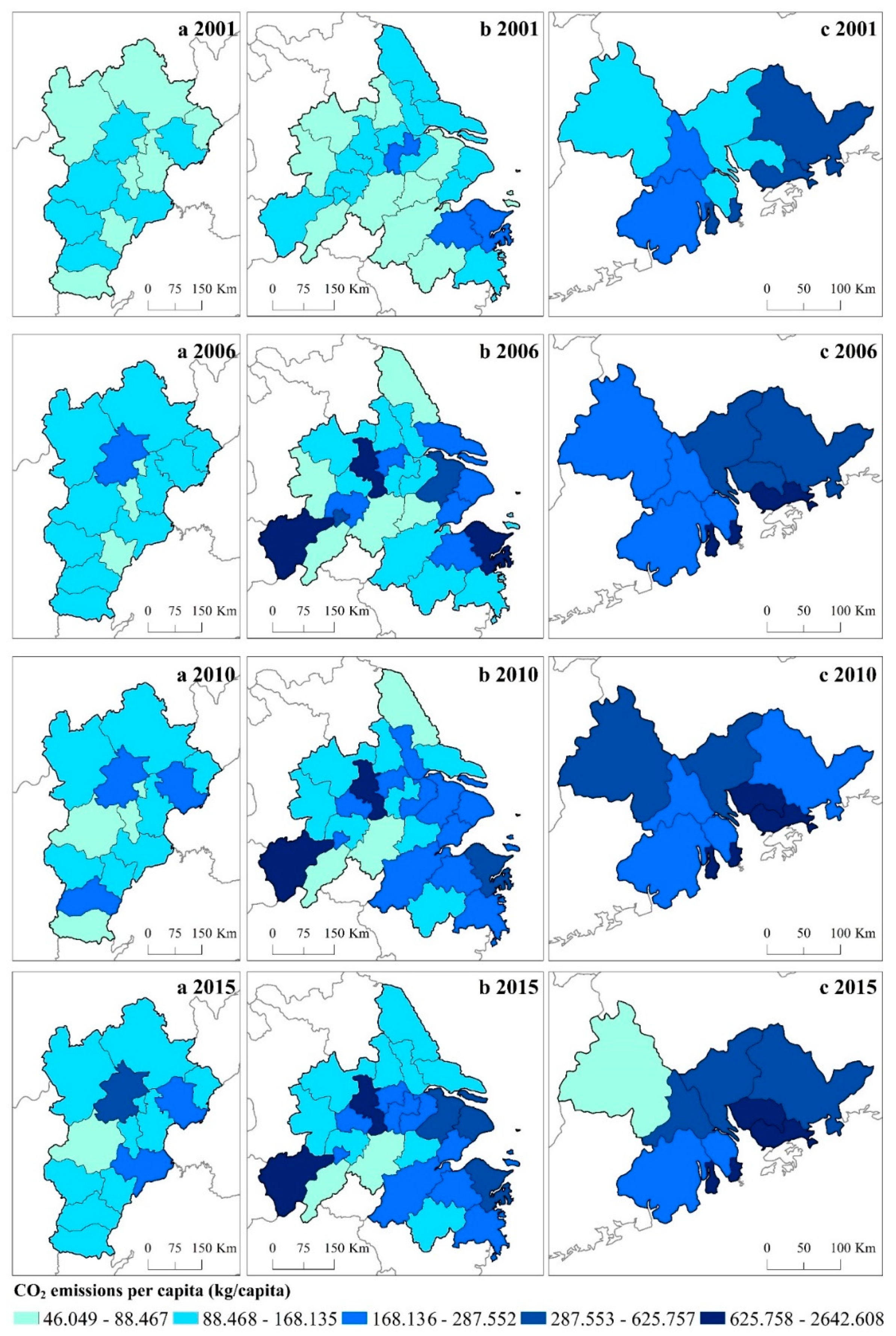₂ emissions in the three urban agglomerations at the city level via the construction of a comprehensive system to capture the effect of urbanization. The findings show that most cities of the three urban agglomerations are at or will enter the stage of exacerbating CO₂ emissions as urbanization progresses, which will place enormous pressure on emissions reduction in China, where urbanization is regarded as a main measure to promote economic development. Therefore, how to maintain a balance between continuing economic growth and reducing CO₂ emissions is directly related to achieving sustainable development in China. Besides, the research results about relationship between CO₂ emissions and urbanization based on different models or data were inconsistent, suggesting that the effect of urbanization on CO₂ emissions is complex and should be further analyzed in future.

The present study demonstrates that for innovation, which were found to exert a positive effect on reducing CO₂ emissions in previous studies such as those by Zhang et al. [17] and Su et al. [36], only significantly decreased CO₂ emissions were observed in the YRD among the three urban agglomerations. Innovation did not have a significant positive and direct effect on reducing CO₂ emissions in the PRD, which is partly because the PRD is an important base of manufacturing and export in the world, and compared with companies in the BTH and YRD, those in the PRD have stronger autonomous innovation ability, while university and scientific research institution innovations are obviously lagging far behind [16]. The former has a greater focus on new technology, products, and facilities to obtain economic benefits rather than environmental profits in the race for economic growth, whereas the latter focuses more on fundamental research, including emission reduction technology [43,44]. Therefore, the high level of innovation did not have a significant or direct contribution to reducing CO₂ emissions in the PRD.

However, the findings in this study indicate that innovation has an indirect and significant positive effect on reducing CO₂ emissions by alleviating the impacts of urbanization on CO₂ emissions in the YRD and PRD. This result is consistent with Liang et al. [27] and Wang [28], who found that technological advantages allow a region to reduce residential and production energy consumption in the process of urbanization. Therefore, for the YRD and PRD, innovation, such as green construction and buildings, new energy and energy-saving transport can effectively reduce energy consumption and improve the energy efficiency of large-scale infrastructure and residential housing construction, the daily life of urban residents, and other activities in the process of urbanization, thereby decreasing CO₂ emissions originating from urbanization. In addition, the intensity of the moderating effect of innovation is positively related to the development level of urbanization, which is probably because in the early stage of urbanization, innovation promotes the speed and scale of urbanization, such as changing the economic structure from agriculture to secondary industry while in the mid-latter period of urbanization, innovation has a significant effect on improving the quality and efficiency of urbanization. In the BTH, however, innovation has neither significantly direct nor indirect effects on reducing CO₂ emissions. One explanation for this finding is that with the exception of Beijing and Tianjin, the cities of the BTH belonging to Hebei Province presented a relatively low level of innovation and urbanization, and the industrial structure of these cities is dominated by heavy industries. Therefore, the development of urbanization will consume considerable energy, but the necessary technology to reduce energy consumption or improve energy efficiency in this process is lacking.

In addition, compared with the research results of Han et al. [37] and Liu et al. [45], who found a significant positive spatial spillover effect on CO₂ emissions because of the demonstration effect, the results presented in this study confirm that there is a significantly negative spatial spillover effect on CO₂ emissions for the three urban agglomerations, which may be related to the indirect transfer of CO₂ emissions from a local city to neighboring cities via the import of high energy-consuming products from neighboring cities because of the close cooperation and trade ties in urban agglomerations. For example, Wu et al. [46] found that household consumption of Beijing, Shanghai and Tianjin highly depend on the flow of products from other regions, and Chen et al. [47] also found that in the BTH, Hebei Province contributes significant energy consumption to Beijing and Tianjin. Another possible reason is that due to the warning effect, local cities will strengthen environmental regulations and governance to reduce energy consumption and CO₂ emissions to avoid public pressure, supervision and evaluations from higher-level authorities when CO₂ emissions increase in neighboring cities [44].

5. Conclusions and Policy Implications

By using city-level datasets on China’s three major urban agglomerations over the 2001–2015 period, this study examines the moderating effect of innovation on influencing the urbanization-CO₂ emissions nexus using a spatial econometric model. Concretely, this study investigates whether innovation tends to attenuate or amplify the positive effect of urbanization on increasing CO₂ emissions and whether there is a spatial spillover effect on CO₂ emissions between cities in urban agglomerations based on a comprehensive evaluation system for measuring the development of urbanization and innovation. The main conclusions are as follows.

Evidence from the empirical analysis indicates that urbanization is a critical factor affecting CO₂ emissions and that CO₂ emissions present a nonlinear relationship with urbanization in the three urban agglomerations. Specifically, CO₂ emissions and urbanization are linked by a U-shaped relationship in the BTH and present an N-shaped and inverted N-shaped pattern in the YRD and PRD, respectively. In particular, for the three urban agglomerations, CO₂ emissions are increasing or will increase with the further development of urbanization.

Innovation has a positive effect on reducing CO₂ emissions for the YRD and a nonsignificant effect on CO₂ emissions in the BTH and YRD. However, when innovation is considered the moderating variable, the regression results with the interaction term between urbanization and innovation suggest that innovation significantly attenuates the positive effect of urbanization on increasing CO₂ emissions for the YRD and PRD. In other words, innovation has an important indirect effect on reducing CO₂ emissions by moderating urbanization.

The spatial econometric model results suggest a significant spatial spillover effect of CO₂ emissions between cities for the three urban agglomerations. For the three urban agglomerations, the CO₂ emissions of a local city have a negative relationship with those of neighboring regions because of the indirect transfer of CO₂ emissions and the warning effect in urban agglomerations. In addition, investment shows a significantly positive effect on reducing CO₂ emissions for the BTH and YRD, respectively. Furthermore, FDI exerts a significantly positive and negative effect on decreasing CO₂ emissions for the BTH and PRD, respectively.

Based on the analysis above, this study proposes the following policies:

Under the pressure of the international community to reduce CO₂ emissions and the positive effect of urbanization on economic development, China must properly handle the complex effect of urbanization in order to reduce CO₂ emissions, while achieving economic growth. Therefore, the quality of urbanization must be improved, and the large flatbread development pattern must be changed. More importantly, the potential of innovation, including new energy, green buildings and facilities as well as efficient management must be further strengthened and fully exploited to reduce the negative impacts of urbanization on CO₂ emissions and promote a low-carbon and sustainable urbanization model, rather than merely slowing the speed of urbanization.

The significantly negative spatial spillover effect of CO₂ emissions on urban agglomerations indicates that it is inappropriate to reduce emissions in one city through unilateral measures without considering the influence of the surrounding cities. Thus, governments and policymakers should establish regional cooperation mechanisms, including a uniform environment management regulation system, a regional industrial deployment and a joint action plan at the urban agglomeration level to reduce overall CO₂ emissions.

Governments should optimize the structure of investment to avoid the waste and overuse of resources, to increase investment in high-technology industries instead of high-energy-consumption and highly polluting industries, and to upgrade equipment and promote technological transformation. Similarly, policymakers should strengthen environmental permitting regulations to increase the quality of foreign capital and to fully leverage the technology spillover effect of FDI to improve energy consumption efficiency.

References

1. Knox, P.L.; McCarthy, L. Urbanization: An Introduction to Urban Geography; Pearson: Boston, MA, USA, 2012. [Google Scholar]
2. Chikaraishi, M.; Fujiwara, A.; Kaneko, S.; Poumanyvong, P.; Komatsu, S.; Kalugin, A. The moderating effects of urbanization on carbon dioxide emissions: A latent class modeling approach. Technol. Forecast. Soc. Chang. 2015, 90, 302–317. [Google Scholar] [CrossRef]
3. Chen, M.X.; Lu, D.D.; Zhang, H. Comprehensive Evaluation and the Driving Factors of China’s Urbanization. Acta Geogr. Sin. 2009, 64, 387–398. (In Chinese) [Google Scholar]
4. Jones, D.W. Urbanization and energy use in economic development. Energy J. 1989, 10, 29–44. [Google Scholar] [CrossRef]
5. Jones, D.W. How urbanization affects energy-use in developing countries. Energy Policy 1991, 19, 621–630. [Google Scholar] [CrossRef]
6. Madlener, R.; Sunak, Y. Impacts of urbanization on urban structures and energy demand: What can we learn for urban energy planning and urbanization management? Sustain. Cities Soc. 2011, 1, 45–53. [Google Scholar] [CrossRef]
7. Parikh, J.; Shukla, V. Urbanization, energy use and greenhouse effects in economic development: Results from a cross-national study of developing countries. Glob. Environ. Chang. 1995, 5, 87–103. [Google Scholar] [CrossRef]
8. Sheng, P.F.; Guo, X.H. The long-run and short-run impacts of urbanization on carbon dioxide emissions. Econ. Model. 2016, 53, 208–215. [Google Scholar] [CrossRef]
9. Ji, X. Ecological accounting and evaluation of urban economy: Taking Beijing city as the case. Commun. Nonlinear Sci. Numer. Simulat. 2011, 16, 1650–1669. [Google Scholar] [CrossRef]
10. Dodman, D. Blaming cities for climate change? An analysis of urban greenhouse gas emissions inventories. Environ. Urban. 2009, 21, 185–201. [Google Scholar] [CrossRef]
11. Liddle, B. Demographic dynamics and per capita environmental impact: Using panel regressions and household decompositions to examine population and transport. Popul. Environ. 2004, 26, 23–39. [Google Scholar] [CrossRef]
12. Poumanyvong, P.; Kaneko, S. Does urbanization lead to less energy use and lower CO2 emissions? A cross-country analysis. Ecol. Econ. 2010, 70, 434–444. [Google Scholar] [CrossRef]
13. Martínez-Zarzoso, I.; Maruotti, A. The impact of urbanization on CO2 emissions: Evidence from developing countries. Ecol. Econ. 2011, 70, 1344–1353. [Google Scholar] [CrossRef]
14. He, Z.X.; Xu, S.C.; Shen, W.X.; Long, R.Y.; Chen, H. Impact of urbanization on energy related CO2 emission at different development levels: Regional difference in China based on panel estimation. J. Clean. Prod. 2017, 140, 1719–1730. [Google Scholar] [CrossRef]
15. Le Quéré, C.; Moriarty, R.; Andrew, R.M.; Canadell, J.G.; Sitch, S.; Korsbakken, J.I.; Friedlingstein, P.; Peters, G.P.; Andres, R.J.; Boden, T.A. Global carbon budget 2015. Earth Syst. Sci. Data 2015, 7, 349–396. [Google Scholar] [CrossRef]
16. Fang, C.L.; Bao, C.; Ma, H.T. Chinese Urban Agglomeration Development Report 2016; Science Press: Beijing, China, 2016. [Google Scholar]
17. Zhang, Y.J.; Peng, Y.L.; Ma, C.Q.; Shen, B. Can environmental innovation facilitate carbon emissions reduction? Evidence from China. Energy Policy 2017, 100, 18–28. [Google Scholar] [CrossRef]
18. Lee, K.; Min, B. Green R&D for eco-innovation and its impact on carbon emissions and firm performance. J. Clean. Prod. 2015, 108, 534–542. [Google Scholar] [CrossRef]
19. Sarr, M.; Noailly, J. Innovation, diffusion, growth and the environment: Taking stock and charting new directions. Environ. Resour. Econ. 2017, 66, 393–407. [Google Scholar] [CrossRef]
20. Wang, Z.H.; Yang, Z.M.; Zhang, Y.X.; Yin, J.H. Energy technology patents–CO2 emissions nexus: An empirical analysis from China. Energy Policy 2012, 42, 248–260. [Google Scholar] [CrossRef]
21. Geels, F.W.; Schwanen, T.; Sorrell, S.; Jenkins, K.; Sovacool, B.K. Reducing energy demand through low carbon innovation: A sociotechnical transitions perspective and thirteen research debates. Energy Res. Soc. Sci. 2018, 40, 23–35. [Google Scholar] [CrossRef]
22. Chiou, T.; Chan, H.K.; Lettice, F.; Chung, S.H. The influence of greening the suppliers and green innovation on environmental performance and competitive advantage in Taiwan. Transport. Res. E-Log. 2011, 47, 822–836. [Google Scholar] [CrossRef]
23. Buchana, A.H.; Honey, B.G. Energy and carbon dioxide implications of building construction. Energy Build. 1994, 20, 205–2017. [Google Scholar] [CrossRef]
24. Camagni, R.; Capello, R.; Nijkamp, P. Towards sustainable city policy: An economy-environment technology nexus. Ecol. Econ. 1998, 24, 103–118. [Google Scholar] [CrossRef]
25. Bulu, M. Upgrading a city via technology. Technol. Forecast. Soc. Chang. 2014, 89, 63–67. [Google Scholar] [CrossRef]
26. Greening, L.A.; Greene, D.L.; Difiglio, C. Energy efficiency and consumption—The rebound effect—A survey. Energy Policy 2000, 28, 389–401. [Google Scholar] [CrossRef]
27. Liang, J.S.; Hong, L.X.; Cai, J.M. The decomposition of energy consumption growth—During the process of China’s urbanization: 1985–2006. J. Nat. Resour. 2009, 24, 20–29. (In Chinese) [Google Scholar]
28. Wang, Q. Effects of urbanisation on energy consumption in China. Energy Policy 2014, 65, 332–339. [Google Scholar] [CrossRef]
29. Huang, J.B.; Liu, Q.; Cai, X.C.; Hao, Y.; Lei, H.Y. The effect of technological factors on China’s carbon intensity: New evidence from a panel threshold model. Energy Policy 2018, 115, 32–42. [Google Scholar] [CrossRef]
30. Jian, X.H.; Huang, K. Empirical analysis and forecast of the level and speed of urbanization in China. Econ. Res. J. 2010, 28–39. (In Chinese) [Google Scholar]
31. Fang, C.L.; Wang, S.J.; Li, G.D. Changing urban forms and carbon dioxide emissions in China: A case study of 30 provincial capital cities. Appl. Energy 2015, 158, 519–531. [Google Scholar] [CrossRef]
32. IPCC. The Fourth Assessment Report of the Intergovernmental Panel on Climate Change; Cambridge University Press: Cambridge, UK, 2007. [Google Scholar]
33. Liu, F.C.; Pan, X.F.; Shi, D.G. Research on the evaluation of regional independent innovation ability based on set pair analysis. China Soft Sci. 2005, 83–91. Available online: http://www.cnki.com.cn/Article/CJFDTotal-ZGRK200511011.htm (accessed on 1 December 2018). (In Chinese).
34. Dietz, T.; Rosa, E.A. Rethinking the Environmental Impacts of Population, Affluence and Technology. Hum. Ecol. Rev. 1994, 1, 277–300. [Google Scholar]
35. York, R.; Rosa, E.A.; Dietz, T. STIRPAT, IPAT and ImPACT: Analytic tools for unpacking the driving forces of environmental impacts. Ecol. Econ. 2003, 46, 351–365. [Google Scholar] [CrossRef]
36. Su, W.S.; Liu, Y.Y.; Wang, S.J.; Zhao, Y.B.; Su, Y.X.; Li, S.J. Regional inequality, spatial spillover effects, and the factors influencing city-level energy-related carbon emissions in China. J. Geogr. Sci. 2018, 28, 495–513. [Google Scholar] [CrossRef]
37. Han, F.; Xie, R.; Lu, Y.; Fang, J.Y.; Liu, Y. The effects of urban agglomeration economies on carbon emissions: Evidence from Chinese cities. J. Clean. Prod. 2018, 172, 1096–1110. [Google Scholar] [CrossRef]
38. Liu, Y.; Yan, B.; Zhou, Y. Urbanization, economic growth, and carbon dioxide emissions in China: A panel cointegration and causality analysis. J. Geogr. Sci. 2016, 26, 131–152. [Google Scholar] [CrossRef]
39. Kang, Y.; Zhao, T.; Yang, Y. Environmental Kuznets curve for CO 2 emissions in China: A spatial panel data approach. Eco. Indic. 2016, 63, 231–239. [Google Scholar] [CrossRef]
40. Elhorst, J.P. Matlab software for spatial panels. Int. Reg. Sci. Rev. 2015, 37, 389–405. [Google Scholar] [CrossRef]
41. Zhang, C.G.; Lin, Y. Panel estimation for urbanization, energy consumption and CO2 emissions: A regional analysis in China. Energy Policy 2012, 49, 488–498. [Google Scholar] [CrossRef]
42. Feng, D.; Li, J. Impacts of Urbanization on carbon dioxide emissions in the three urban agglomerations of China. Resour. Environ. Yangtze Basin 2018, 27, 2194–2200. (In Chinese) [Google Scholar]
43. Li, B.; Zhao, X.H. Economic structure, technological progress and environmental pollution: Based on the analysis of industrial data in China. J. Financ. Econ. 2011, 37, 112–122. (In Chinese) [Google Scholar]
44. Shao, S.; Li, X.; Cao, J.H.; Yang, L.L. China’s economic policy choices for governing smog pollution based on spatial spillover effects. Econ. Res. J. 2016, 73–88. Available online: http://www.cnki.com.cn/Article/CJFDTotal-JJYJ201609007.htm (accessed on 1 December 2018). (In Chinese).
45. Liu, Y.; Xiao, H.W.; Lv, Y.K.; Zhang, N. The effect of new-type urbanization on energy consumption in China: A spatial econometric analysis. J. Clean. Prod. 2017, 163, S299–S305. [Google Scholar] [CrossRef]
46. Wu, S.M.; Lei, Y.L.; Li, S.T. CO2 emissions from household consumption at the provincial level and interprovincial transfer in China. J. Clean. Prod. 2019, 210, 93–104. [Google Scholar] [CrossRef]
47. Chen, W.M.; Wu, S.M.; Lei, Y.L.; Li, S.T. Interprovincial transfer of embodied energy between the Jing-Jin-Ji area and other provinces in China: A quantification using interprovincial input-output model. Sci. Total Environ. 2017, 584, 990–1003. [Google Scholar] [CrossRef] [PubMed]
Figure 1. The relationship among urbanization, innovation, and CO2 emissions. (a) Direct effect of urbanization and innovation. (b) Innovation as a moderating variable. (c) Urbanization, innovation and CO2 emissions.
Sustainability 11 01633 g001
Figure 2. Geographic location of the three urban agglomerations.
Sustainability 11 01633 g002
Figure 3. Time variations in average CO2 emissions per capita in the three urban agglomerations.
Sustainability 11 01633 g003
Figure 4. CV variations in CO2 emissions per capita in the three urban agglomerations.
Sustainability 11 01633 g004
Figure 5. The spatial distribution of CO2 emissions of the BTH: (a), the YRD (b) and the PRD (c) in 2001, 2006, 2010 and 2015.
Sustainability 11 01633 g005
Figure 6. The variation in urbanization in the three urban agglomerations from 2001 to 2015.
Sustainability 11 01633 g006
Figure 7. CV variation of urbanization in the three urban agglomerations from 2001 to 2015.
Sustainability 11 01633 g007
Figure 8. The variation in innovation in the three urban agglomerations from 2001 to 2015.
Sustainability 11 01633 g008
Figure 9. CV variation of innovation in the three urban agglomerations from 2001 to 2015.
Sustainability 11 01633 g009
Figure 10. The relationship between urbanization and CO2 emissions in the three urban agglomerations.
Sustainability 11 01633 g010aSustainability 11 01633 g010b
Figure 11. The moderating effect of innovation in the three urban agglomerations.
Sustainability 11 01633 g011