Disaggregation Method of Carbon Emission: A Case Study in Wuhan, China

Abstract

Urban areas contribute significant carbon emissions. Evaluating and analysing the spatial distribution of carbon emissions are the foundations of low-carbon city development and carbon emissions reduction. In this study, carbon emission inventory was first constructed and carbon emissions in Wuhan were estimated on the basis of energy consumption. Second, the spatial distribution models of carbon emissions in different sectors were developed on the basis of the census of the Wuhan geographical conditions data and other thematic data. Third, the carbon emission distribution in Wuhan was analyzed at the central urban, functional, new urban, built-up, and metropolitan development area scale. Results show that the industry sector emits most of the carbon emissions in Wuhan, followed by the residential population. Carbon emissions in the metropolitan development area can stand for the true carbon emissions in Wuhan. Thus, a geographically weighted (GW) model was adopted to analyze the correlation coefficients between economical-social factors (gross domestic product, population density, road density, industrial land and residential land) and carbon emissions in the metropolitan development area. Comparisons with other studies show that the disaggregation method we proposed in this work, especially the adoption of geographical condition census data, can reflect the spatial distribution of carbon emissions of different sectors at the city scale.

1. Introduction

Cities are the major drivers of global greenhouse gas (GHG) emissions. The rapid growth of urban GHG emissions is the main reason for the increase of global GHG emissions [1,2]. Cities account for less than 1% of the Earth’s landmass but concentrate more than half of the world’s population, consume approximately 75% of the world’s energy, and contribute 70%–80% of global GHGs [2,3]. Global carbon emissions have been significantly affected by the increase in urban population with the high-speed development of global urbanization [4]. Therefore, low-carbon economy development and city construction become inevitable actions for all countries in order to face the climate challenge and promote sustainable urban development. In June 2007, the Chinese government formally released “China’s National Climate Change Programme”, which clearly defined the principles, objectives, and measures to combat climate change. At the Copenhagen Climate Change Conference in December 2009, the Chinese government promised to reduce the carbon intensity (carbon emissions per unit gross domestic product [GDP]) to 40%–50% below 2005 levels by 2020.

The foundation of low carbon policy making is the accurate estimation of carbon emissions. The World Resources Institute divides carbon emissions into three categories: Scope 1 emission is the direct carbon emission within the city; Scope 2 refers to the indirect carbon emission caused by the purchase and usage of energy, steam, and heating/cooling; and Scope 3 emission indicates the carbon emission that occurs outside the city due to the activities within the city (Scope 3) [5]. Under the leadership of the Intergovernmental Panel on Climate Change (IPCC), Center for Global Engagement (CGE), C40 cities, and other agencies and organizations, numerous cities in the world have established their own carbon inventories [6,7,8,9,10,11]. Some major cities, such as New York, Tokyo, Chicago, and London, have evaluated carbon emissions on the basis of the carbon inventories [5,12]. Because Scope 3 emission is difficult to define, most studies concentrate on Scope 1 and Scope 2 emissions. This study focuses on the Scope 1 emission.

It is also crucial to benchmark carbon emission estimates and spatial-temporal carbon emission analysis from different sources at multiple administrative levels, for example, the national, regional, metropolitan, and precinct scales. Precincts are a microcosm of cities. Carbon assessment at the precinct level can lead to mapping and reducing the carbon signature of the entire urban system, as well as support government policy-making. Precinct-scale assessment is expected to lead urban design and planning with carbon assessment and decision support at the early stage [13,14]. Different areas play different roles in city development and make different contributions to carbon emissions. Urban areas tend to offer easier access to more energy-intensive fuels, as well as electricity, and also have higher population density and limits on space, concentrating emission sources [5]. Low-density rural and suburban areas can be less susceptible to urban heat islands and traffic congestion, but also tend to suffer from greater efficiency losses associated with the longer transmission of electricity, more vehicle miles travelled, and the inability to rely on district heating and combined heat and power systems. Moreover, suburban and sprawling communities are more likely to have single-family detached houses and to live in bigger houses, both leading to higher energy use and grater carbon emissions [5,15,16].

The mostly commonly used spatial carbon emission analysis can be generally categorized into top-down and bottom-up approaches. Population density, the Defense Meteorological Satellite Program’s Operational Linescan System (DMSP/OLS) nighttime light image, point emission sources and other data are widely used to estimate carbon emissions at different scales [17,18,19,20]. Several carbon emission datasets are also available at different resolutions. The Emission Database for Global Atmospheric Research (EDGAR V4.3) [21] and the Fossil Fuel Data Assimilation System (FFDAS) [22,23] have CO2 emissions data at 0.1° × 0.1° (roughly 10 km × 10 km) spatial resolution. Based on the first China pollution source census, China high resolution emission gridded data (CHRED) provided 10 km × 10 km spatial resolution of CO2 emissions estimation of China with data from 1.58 million industrial enterprises [24].

Although much work has been done in this field, there are still several barriers hindering the uptake of multiple level evaluation, and these barriers include system boundary definition, data availability, dynamic inter-building effects contributed by urban morphology, uncertain preferences for occupants’ life-style, integrated modelling and the less standardized production process of precinct objects caused by their unique characteristics [25,26,27,28,29]. Moreover, the literature research and datasets are more suitable for large scale carbon emission evaluation, such as at the regional and provincial scale, and have difficulties in reflecting the spatial pattern of carbon emission in cities.

In this paper, we first introduced the study area and data, especially the geographical conditions census data. Then, we introduced the carbon emissions disaggregation models for different sectors, including industry, agriculture, residential living, waste disposal and transportation. Land coverage, geo-graphical units, thematic data and statistical data from the census of national geographical condition data were adopted to disaggregate the carbon emissions at street scale, which is the finest administrative level in China. We analyzed characteristics of carbon emissions in different areas and sectors in Wuhan. We also discussed the spatial correlation coefficients between economical-social factors (gross domestic product, population density, road density, and land-use structure) and carbon emissions in the metropolitan development area. Finally, we compared our data and methods with other studies.

2. Research Area and Data

2.1. Research Area

Wuhan is strategically located inland of central China (Figure 1a) and has been called the “thoroughfare to nine provinces” since ancient times. Wuhan is undergoing a major construction and development stage. Urban construction, especially infrastructure construction, has a strong carbon-locking effect. Moreover, the industrial structure of Wuhan, as a heavy industry city, means that great energy consumption is necessary for economic development.

Wuhan has 17 districts and 183 streets (townships), which can be classified into central, functional, and new urban areas in accordance with the functional orientation (Figure 1b). The central area includes the Jiang’an, Jianghan, Qiaokou, Hanyang, Wuchang, Qingshan, and Hongshan Districts, in which modern services constitute the dominant industry. The central area is known as the first echelon of urban development. The functional zone includes the Wuhan Economic and Technological Development Zone (WETDZ), East Lake High-Tech Development Zone (ELHDZ), East Lake Ecotourism Scenic Zone (ELESZ), and Wuhan Chemical Industrial Park (WCIP). The functional zone is known as the second echelon of urban development, in which advanced manufacturing, strategic emerging industries, and modern logistics are the leading industries. The new urban area includes the Dongxihu, Caidian, Jiangxia, Huangpi, Xinzhou, and Hannan Districts, where green manufacturing is the leading industry.

In addition to the above-mentioned three levels, Wuhan can also be divided into different zones in accordance with management purposes. The built-up area is the most developed area with the highest population density and the most developed economy and society in Wuhan. The metropolitan development area covers the central urban area, a part of the functional and new urban areas [30]. Figure 1c shows the spatial location and distribution of the built-up and metropolitan areas. In order to characteristics of carbon emissions in different areas, we use streets as the basic calculation unit and analyze carbon emissions at the city, district, central urban area, functional area, new urban area, built-up area, and metropolitan development area scale.

2.2. Data Sources

2.2.1. Carbon Emission Inventory

The carbon emission inventory in Wuhan was constructed with reference to the GHG inventory in major cities home and abroad [9,10,31], as well as the economic features in Wuhan (

Table 1. Wuhan carbon emission inventory. Sector is the major carbon emission sector in Wuhan. Category refers to the energy consumption or materials which would cause carbon emission.

Sector	Category	Carbon Emission Factors	Reference Source
Energy consumption	Coal	0.7559 t/t	T.O. West, American Oak Ridge National Laboratory
	Coke	0.855 t/t	American Oak Ridge National Laboratory
	Crude oil	0.5857 t/t	IREEA
	Aviation gasoline	0.6185 t/t	IPCC
	Motor gasoline	0.5538 t/t	China Agricultural University School of Biology
	Diesel oil	0.5927 t/t	Dubey
	Kerosene	0.5714 t/t	IPCC
	Refinery gas	0.4602 t/t	IPCC
	Liquefied petroleum Gases	0.5042 t/t	IPCC
	Coke oven gas	0.3548 t/t	IPCC
	Electricity	Converted standard coal	IPCC
Industrial Production	Soda ash	0.1380 t/t	T.O. West, American Oak Ridge National Laboratory
	Crude iron	0.1100 t/t	IREEA
	Crude steel	0.1100 t/t	IPCC
	Rolled Steel	0.1100 t/t	China Agricultural University School of Biology
	Cement	0.4083 t/t	Dubey
	Flat glass	0.2100 t/t	IPCC
Agriculture	Chemical fertilizer	0.89 kg/kg	T.O. West, American Oak Ridge National Laboratory
	Pesticides	4.93 kg/kg	American Oak Ridge National Laboratory
	Plastic sheeting	5.18 kg/kg	IREEA
	Diesel oil	0.59 kg/kg	IPCC
	Irrigation	25.00 kg/Cha	Dubey
Residential living	Electricity	Converted standard coal	IPCC
	Natural gas
Waste disposal	Domestic waste treatment	0.35 t/t	American Oak Ridge National Laboratory
Transportation	Bus	106.42 kg/100 km	Ministry of Transport of the People’s Republic of China
	Taxi	22.26 kg/100 km
	Private car	19.59 kg/100 km
	Motorcycle	6.68 kg/100 km
	Big truck	106.42 kg/100 km
	Van	53.20 kg/100 km

Note: The unit XX t/t means emission of XX ton carbon with each ton’s consumption. The unit XX kg/kg means emission of XX kilogram carbon with each kilogram’s consumption. The unit XX kg/Cha means emission of XX kilogram carbon with each hectare’s farming. The unit XX kg/100 km means emission of XX kilogram carbon with each 100 km’s driving.

). Scope 2 and Scope 3 carbon emissions are difficult to define. Since carbon emission inventory construction was beyond the scope of this study, we only considered Scope 1 carbon emissions in the inventory, which includes industrial production (industrial energy consumptions and producing procedures), agricultural production, waste disposal, residential living, and transportation carbon emissions. Agricultural emissions involve those from irrigation, fertilization and pesticides. Waste disposal carbon emissions are from waste treatment processes. Residential living carbon emissions mainly include emissions from household electricity and gas consumption. Transportation carbon emissions mainly refer to carbon emissions from vehicles driving inside Wuhan, since cross-frontier transportation is difficult to define.

2.2.2. Census of Geographical Conditions Data

Under the unified arrangement of Chinese government, Wuhan carried out the first geographical conditions census from 2013 to 2015. In order to accurately reflect the geographical conditions, the Chinese government designed a very strict quality control system. There are technical and procedural regulations concerning every step of data collection, including filed survey, data checking, data entry to the database and statistical analysis, etc. Land coverage data, geographical element data, thematic data products and other products must pass indoor and field quality check. For example, the errors between land coverage map-spot and 0.5 m resolution remote sensing images must be less than 5 pixels (i.e., the overall precision of land coverage data is better than 2.5 m). After two years of work, we produced 83.7 million land coverage map-spots, 210.1 million geographical element records, and 621 types of thematic data in Wuhan.

Table 2. List of Wuhan geographical conditions census data used in this study. Category refers to the product from the census of geographical conditions.

Category	Feature	Attributes Used
Land coverage	Land coverage data	Type
Road networks	Centerline of highway	Type, length, width, road grade
	Centerline of city road
	Centerline of country road
Geographic units	District (county) boundaries	Location, area
	Street (township) boundaries
	Industrial enterprises
	Residential areas
Thematic data	Survey of population	Population
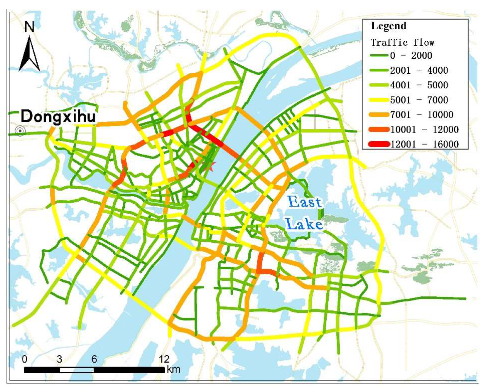
	Traffic flow	Annual traffic flow of main road
Statistical data	Economic and social data	GDP, Gross industrial output value above designated size, irrigation, consumption of materials in agricultural production, vehicle holdings and driving distance

presents the Geographical Conditions Data used in our study.

Statistical data is from the Wuhan Statistical Yearbook 2015, Wuhan Census of Geographical Conditions Report, and Wuhan Transportation Development Annual Report 2015 et al. Population distribution data is from the survey of “Actual Housing and Actual Population” in Wuhan in 2015.

3. Research Methods and Models

3.1. Total Carbon Emissions Estimation

According to the IPCC and Guideline of GHGs inventory for provinces of China [6,7], carbon emissions can be calculated on the basis of energy consumption using the following formula:

$$E={{\displaystyle \sum }}^{\text{}}{E}_i={{\displaystyle \sum }}^{\text{}}{T}_i \times {\delta }_i$$

(1)

In Equation (1), E refers to the carbon emissions and $E_i$ indicates carbon emission of different sectors, including industry (consisting of energy consumption and industrial producing), agriculture, residential living, waste disposal, and transportation. $T_i$ is the activity level, and ${\delta }_i$ denotes the carbon emission factor.

To evaluate carbon emissions quantitatively, the carbon emission intensity and carbon emission per capita are defined. The formula is shown in Equation (2):

$$C_j=\frac{E_j}{S_j},e_j=\frac{E_j}{P_j}$$

(2)

In this formula, $C_j$ and $e_j$ represent the carbon intensity and emission per capita of the jth region, respectively. $E_j$ is the total carbon emissions, $S_j$ stands for the area, and $P_j$ refers to population.

3.2. Dissageration Method of Carbon Emissions

To disaggregate carbon emissions, scale factors of carbon emissions from different sectors were first analyzed. Then, disaggregation models of single and multi-effect factors, combined with the geographical condition data, were developed accordingly (Figure 2). In order to serve the low-carbon city development, the street is selected as the basic statistical unit. It’s worth mentioning that the disaggregation can be done at other scales, since the geographical condition data provides detailed geo-information data.

3.2.1. Single Scale Factor Model

Industrial carbon emissions and waste disposal carbon emissions are disaggregated using a single scale factor model, as defined in Equation (3).

$$C_n^i=\frac{S_n^i}{{{\displaystyle \sum }}_{n=1}^N{S}_n^i}{C}_i$$

(3)

For industrial carbon emissions, $C_n^i$ represents the industrial carbon emissions of the nth street in the ith district, which is evaluated using Equation (1). $S_n^i$ is the scale factor in the nth street and it refers to the industrial land area. $S_n^i$ is calculated using the industrial land from the geographical condition data, which is composed of 4997 manufacturing enterprises. For waste disposal carbon emissions, $S_n^i$ refers to the population and is calculated using population survey data.

3.2.2. Multi Scale Factors Model

Agriculture, residential living and transportation carbon emissions are disaggregated using multi scale factors models, as defined in Equation (4).

$$C_n^i=\frac{S_n^i \times P_n^i}{{{\displaystyle \sum }}_{n=1}^N{S}_n^i \times P_n^i}{C}_i$$

(4)

In the formula, $C_n^i$ is the carbon emission of the nth street in the ith district. $S_n^i$ and $P_n^i$ denote the factors of the nth street. $C_i$ signifies the total carbon emissions of the ith district. For agricultural carbon emissions, $S_n^i$ and $P_n^i$ represent the cultivated land area and population in the nth street. They are calculated using land coverage data and population survey data, respectively. For residential living and waste disposal carbon emissions, $S_n^i$ and $P_n^i$ represent the residential living area and population. Residential living area is calculated using geographical units, which is composed of 6049 residential areas in Wuhan. For transportation carbon emissions, $S_n^i$ and $P_n^i$ refer to road areas and traffic flow, respectively. Traffic flow data [32] is demonstrated in Figure 3. If the traffic flow data is missing, the buffer zone of the total population in the 2 km around the road is used as an auxiliary factor to determine the weight of roads for transportation carbon emission.

3.2.3. Geographical Weighted Statistics Model

To analyse the local influences of social-economic factors on carbon emissions, we introduce geographically weighted (GW) summary statistics techniques [33,34]. GW summary statistics provides local views in exploratory spatial data analysis [33]. The GW statistics model is defined in Equations (5)–(8).

$$\overline{x}\left(u_i,v_i\right)=\frac{{{\displaystyle \sum }}_j{x}_j{w}_{ij}}{{{\displaystyle \sum }}_j{w}_{ij}}$$

(5)

$$\mathrm{SD}\left(u_i,v_i\right)=\sqrt{\frac{{{\displaystyle \sum }}_j{\left(x_j-\overline{x}\left(u_i,v_i\right)\right)}^2{w}_{ij}}{ {{\displaystyle \sum }}_j{w}_{ij}}}$$

(6)

$$\mathrm{Cov}\left(u_i,v_i\right)=\frac{{{\displaystyle \sum }}_j\left[\left(x_j-\overline{x}\left(u_i,v_i\right)\right)\left(y_j-\overline{y}\left(u_i,v_i\right)\right)\right]}{ {{\displaystyle \sum }}_j{w}_{ij}}$$

(7)

$${\rho }_{x,y}\left(u_i,v_i\right)=\frac{Co{v}_{\left(x,y\right)}\left(u_i,v_i\right)}{S{D}_x\left(u_i,v_i\right)S{D}_y\left(u_i,v_i\right)}$$

(8)

$\overline{x}\left(u_i,v_i\right)$, $\mathrm{SD}\left(u_i,v_i\right)$,$\mathrm{Cov}\left(u_i,v_i\right)$ and ${\rho }_{x,y}\left(u_i,v_i\right)$ are GW mean, standard deviation, covariance and correlation coefficient, respectively. $\left(u_i,v_i\right)$ represents the spatial coordinate at location i, $x$ and $y$ refer to attributes, and $w_{ij}$ is the weight calculated via a kernel function. A kernel function is defined as a decreasing function of distance with values ranging from 0 to 1. In this study, we selected the Bi-square function [33,34,35] to calculate $w_{ij}$.

4. Results and Discussions

4.1. Carbon Emission Characteristics in Wuhan

According to our results, in 2015, the total carbon emission in Wuhan is 120 million tons, the carbon emission per capita is 11.3 tons, and the average intensity of carbon emission is 14,000 tons/km². Industrial, transportation, residential living, and agriculture emissions are the main sources of carbon emissions, with proportions of 87.58%, 5.75%, 5.63%, and 0.18%, respectively (Figure 3). The study from the World Bank shows that the main carbon emission source in China’s big cities is industrial emission, whereas the main carbon emission sources in developed countries are energy supply, transportation, and architecture. Wuhan’s carbon emission has typical Chinese characteristics.

Figure 4 and Figure 5 shows the spatial distribution of carbon emissions in Wuhan. The total carbon emission, carbon emission intensity, and carbon emission per capita at district and street scale are illustrated from top to bottom and from left to right.

At the district scale, the total carbon emission, carbon emission intensity, and carbon emission per capita show different patterns. The gross domestic product (GDP) of the secondary industry in Hanyang District is 64.19 billion yuan in 2015, accounting for 18.90% of Wuhan’s GDP. The secondary industry GDP in Dongxihu District is 47.694 billion yuan, accounting for 14.04% of the city’s GDP. The concentration of large enterprise, large energy consumptions of these two districts result in enormous carbon emissions. ELESZ has the least carbon emissions, followed by WLHDZ and Jianghan District, in which residential living is the dominant carbon emission type. Carbon emission intensities in Hanyang, Qiaokou, and Jianghan Districts are considerably larger than those in other districts. Although the carbon emission of Jianghan and Qiaokou Districts ranked 15th and 11th among 17 districts, their carbon emissions intensity are the largest, with more than 100,000 tons/km². The carbon emission intensities of ELHDZ and Huangpi District are the lowest, less than 5000 tons/km². The emission per capita in WCIP, which is 138.68 tons/km², is significantly higher than those in other districts. The emissions per capita of Hanyang and Dongxihu Districts are approximately 30 tons/person, which ranks second. Other districts’ carbon emissions per capita are less than 25 tons/person, in which the least is ELHDZ with carbon emissions of only 2.52 tons/person.

At the street scale, the spatial distribution of carbon emission in the city can be reflected more intuitively. Generally speaking, streets of Qingshan District and WCIP have significantly higher emissions than those of other districts. Carbon emissions in Bajifu Street and Wuhan Iron and Steel Company are significantly larger than those of other streets. Most of the carbon emissions are concentrated in the functional areas between the second and third belt highways. The emission intensity shows a decreasing trend from the central to the rural area, while the carbon emission per capita presents a low–high–low trend from the city center to the rural area. Many industry concentrated streets often with lower population, making their emissions per capita significantly higher than other streets. The carbon emission per capita of the central urban area is considerably lower than those of other regions due to its high population concentration.

4.2. Carbon Emission Characteristics of Different Regions

To reflect carbon emission characteristics of different agglomerations, this study mainly analyzed carbon emissions and social-economic indicators in the central city, functional area, new urban area, built-up area, and metropolitan development area (

Table 3. Comparison of carbon emissions and social-economic indicators in Wuhan.

	Central City	Functional Area	New Urban Area	Built-up Area	Metropolitan Development Area
Area ratio	7.49%	10.39%	82.12%	6.77%	38.18%
Population ratio	57.51%	8.25%	34.24%	71.70%	77.61%
Population density	9499.39	982.3	515.68	13096.63	2514.39
Agricultural land ratio	1.23%	6.67%	92.08%	0.24%	22.80%
Road length ratio	10.98%	11.87%	77.15%	16.57%	49.47%
Road density	3.28	2.56	2.1	5.47	2.89
Residential land ratio	55.28%	14.24%	30.49%	76.48%	94.75%
Industrial land ratio	17.98%	20.43%	61.59%	43.69%	80.20%
Carbon emission ratio	42.84%	9.12%	48.04%	29.47%	86.47%
Industrial carbon emission ratio	43.00%	8.46%	48.54%	28.93%	86.39%
Agricultural carbon emission ratio	1.05%	6.30%	92.65%	1.20%	23.16%
Residential living carbon emission ratio	41.70%	18.71%	39.59%	38.04%	89.39%
Transportation carbon emission ratio	43.00%	8.46%	48.54%	28.93%	86.39%
Waste disposal carbon emission ratio	41.70%	18.71%	39.59%	38.04%	89.39%
Carbon emission per capita	9.07	12.53	15.9	4.65	12.63

Note: The unit for population density is people/km², unit of road density is km/km², unit of carbon emission per capita is ton/person.

).

The city centre of Wuhan contains 57.51% of the city’s population within 7.48% of the city’s area. Due to the high population concentration, residential land area is significantly higher than other parts, which accounts for 55.28% of the total residential land. Residential energy consumptions and waste disposal amounts are also large. Carbon emissions account for 43% and 41.70% of the total emissions. The average road density is 3.28 km/km². The city road densities in Jianghan and Qiaokou Districts, 6.20 and 5.12 km/km², are considerably larger than those in other districts in the central area. The high-density road network, population aggregation, and heavy traffic flow make transportation carbon emissions in the city center account for 43% of the city’s total carbon emission. The industrial carbon emission patterns are relatively different, due to various development strategies. For example, Hanyang District has priority in manufacturing, and Qingshan District is dominated by Wuhan Iron and Steel Company, while Jianghan District is dominated by modern business industry. The industrial carbon emissions in Hanyang District are 7.6 times that in Jianghan District and 3.13 times that in Qingshan District.

The new urban area is larger than the central area and the population is relatively scattered. Carbon emissions are still dominated by industrial carbon emissions, accounting for 88.49% of all emissions, followed by transportation and residential living carbon emissions. The mileage of roads accounts for 77.51% of the city’s road, which are mainly rural roads with light traffic pressure, but the transportation carbon emissions only account for 48.54% of total transportation carbon emissions. Further, 92.08% of agricultural land distributed in the new urban area and the new urban area contributes 92.65% of agricultural carbon emissions. Carbon emissions and social-economic indices of the functional area are also higher than those of the new urban area, but lower than those of the central city.

The built-up area has a higher population density, road network density, residential area ratio, and industrial land ratio than the central city. Carbon emissions in the built-up area are still dominated by industrial carbon emissions, but the total carbon emissions and carbon emissions per capita are significantly lower than other areas. The reason is that the built-up area is the construction-completed area with the most dense population and the highest floor area ratio. The industrial enterprises in this area are mainly light industry and service-oriented enterprises, which generally have less carbon emissions.

The metropolitan development area is the major construction area in Wuhan. This region contains 77.61% of the population, 94.75% of residential areas, 80.20% of industrial land, 49.47% of road network and contributes 86.67% of carbon emissions in Wuhan. The carbon emissions per capita is 12.63 tons, which is significantly higher than those of the city center and built-up areas. The allocation and distribution of industry in the metropolitan development area is the epitome of Wuhan’s present stage, and its carbon emissions can be regarded as the real carbon emission level of Wuhan.

4.3. Carbon Emission Characteristics in Different Sectors

We also discussed carbon emission characteristics in different sectors. Figure 6 shows carbon emissions and emission intensity of different sectors at street scale.

Industrial and transportation carbon emissions in Wuhan show a similar circle distribution trend from the center to the periphery. Industrial carbon emissions and intensity in the city center are generally low, and high carbon emissions are concentrated in the functional areas, especially areas between the second and third belt highways. On one hand, the reason lies in the urban development planning and functional orientation of each district. On the other hand, these regions have significant geographical location advantages, such as abundant raw materials and labor resources, and convenient transportation. Transportation carbon emission intensity in Hankou District is generally higher than that in Wuchang and Hanyang Districts, because the density of the urban road network is considerably higher. In addition, some areas in Qingshan District and WCIP have large transportation carbon emissions. The reason is that large enterprises, such as Wuhan Iron and Steel Company, have large transportation needs, resulting in high traffic carbon emissions. Residential living carbon emissions and waste disposal carbon emissions in Wuhan have a similar distribution tendency, which are both closely related to population distribution. The agricultural production carbon emission tends to decrease from the periphery to the city center. The areas with high carbon emission and emission intensity are mainly concentrated in the new urban area.

4.4. GW Spatial Correlation Analysis

In this section, we explore the relationships between carbon emissions and social-economic indicators via GW correlation coefficients with the GWmodel package in R. Summaries of GW correlation coefficients are demonstrated in

Table 4. Summaries of GW correlation coefficients between social-economic indicators and carbon emissions.

Variables	Correlation Coefficient	Min	Max	Mean	Median
Population density	−0.225	−0.745	0.647	−0.213	−0.307
GDP	0.543	−0.033	0.941	0.637	0.718
Road denstiy	−0.147	−0.704	0.630	−0.122	−0.202
Residential land area	0.202	−0.162	0.912	0.423	0.415
Industrial land area	0.607	0.174	0.988	0.766	0.810

Notes: Min stands for the minimum value, Max stands for the maximum value, Mean stands for the average value, Median stands for the median value of all the GW correlation coefficient in the metropolitan development area.

. Density plots are illustrated in Figure 7.

Carbon emissions are closely correlated with GDP, industrial land area and population density. Correlations with road density and residential land area are relatively small. Figure 8 shows spatial distribution of GDP (Figure 8a), GW correlation of GDP (Figure 8b), industrial land area (Figure 8c), GW correlation of industrial land area (Figure 8d), population density (Figure 8e) and GW correlation of population density (Figure 8f).

Carbon emissions in the metropolitan development area are positively correlated with GDP, which means the higher the GDP, the more carbon emissions. The correlation is distinctly high at the central area, and this means that carbon emissions in this region would increase significantly with the increase of GDP.

For the industrial land, since the industry sector is the major source of carbon emissions in Wuhan, carbon emissions are positively correlated with the industrial land area in most streets. Streets in the functional area generally have higher industrial land areas and carbon emissions. The increase of industrial land areas will also raise carbon emissions, but the degree of improvement is less than that in the central area.

For the population density, the GW correlation distribution shows very interesting trend. The population density in the central area is obviously higher than other regions. However, the more people gathered at the central area, the less carbon emissions in this region. The reason for this phenomenon is that increasing population will occupy industrial land, which will greatly reduce industrial carbon emission. For the periphery area of metropolitan development area, population density is positively correlated with carbon emissions. There is adequate unused but suitable land in this region, increasing population density would improve the land utilization rate, which would also increase carbon emissions.

4.5. Comparisons with Other Studies

The latest released EDGAR 4.3.3 gridded emissions cover 1970–2013 time series, FFDAS datasets cover 1997–2010 time series, and CHRED release carbon emission dataset in 2007 and 2012. Due to data unavailability, we can’t make quantitative comparisons. Therefore, we analyze differences in methods and data used in these datasets and our work.

Both EDGAR and FFDAS datasets use fossil fuel data from IEA statistics (http://www.iea.org/) to evaluate fossil carbon emissions. CHRED evaluate fossil fuel carbon emissions using official statistical yearbooks, which is more accurate for China. Then geo-information data is used to disaggregate carbon emissions at different resolutions. EDGAR uses the location of energy and manufacturing facilities, road networks, shipping routes, human and animal population density and agricultural land use. FFDAS utilizes population, per capita GDP, energy intensity of the economy, carbon intensity of energy production, nightlights, and emissions from listed power stations as control variables for the application of spatial operators. CHRED uses industrial facilities, landfills and wastewater treatment plants.

All these datasets are derived using bottom-up methods and the accuracy is determined by the geo-information data. Due to the geo-information data availability, EDGAR, FFDAS and CHRED datasets are more suitable for large scale carbon evaluation, such as the national and provincial scale. For example, they omit traffic flow and traffic congestion in city. At the city and street scales, our method needs much finer geo-information data in order to better reflect carbon emission characteristics.

5. Conclusions

In this study, we construct a carbon inventory in Wuhan based on the IPCC inventory and evaluated carbon emissions in 2015. On the basis of the geographical national conditions data, carbon emission disaggregation models for different sectors were proposed. We analyzed carbon emission characteristics at different regions and in different sectors, especially the spatial correlations at the metropolitan development area. Comparisons were made to prove the feasibility and effectiveness of the geographical conditions data in the application of carbon emissions. With the continuous accumulation of geographical conditions monitoring data in the future, spatial-temporal changes in of carbon emissions can be recognized, which would help evaluate low-carbon city development. The main conclusions are as follows:

(1) Main carbon emissions in Wuhan are still from industrial production, whereas living and transportation carbon emissions account for a relatively small part, indicating a large gap with developed countries. The carbon emission per capita in Wuhan is 11.31 tons/person, which is considerably higher than the national average level. Therefore, industrial restructuring and energy consumption optimization will take time to be achieved.

(2) The carbon emission patterns in all regions of Wuhan vary significantly. Carbon emissions from residential living and transportation in the center area are palpably higher than those in other regions, while industrial carbon emissions in the new urban areas are significantly higher. Moreover, emissions from various sectors in the functional areas are relatively balanced. The metropolitan development area can better represent the carbon emission characteristics of Wuhan than other regions. The spatial correlation analysis show that carbon emissions are positively correlated with GDP and industrial land, and negatively correlated with population density in Wuhan.

Evaluation and disaggregation of carbon emissions at the city scale remain great challenges of significant interest in the carbon emissions field. Although some exploratory works have been conducted in this study, several problems need to be further addressed.

(1) The census of geographical conditions has a strict data collection standard. Some land coverage less than the minimum acquisition area indices is ignored, which might cause errors in the spatialization process.

(2) This study considers the Scope 1 emission but not the Scope 2 and Scope 3 emissions, and therefore may underestimate carbon emissions. For example, carbon emissions caused by cross-boundary transportation and outbound transportation are not included.

References

- OECD. Cities and Climate Change; OECD Publishing: Paris, France, 2010. [Google Scholar]
- IEA. Cities, Towns & Renewable Energy; IEA: Paris, France, 2009. [Google Scholar]
- UN-HABITAT. State of the World’s Cities 2010/2011: Bridging the Urban Divide; UN-HABITAT: Nairobi, Kenya, 2010. [Google Scholar]
- O’Neill, B.C.; Dalton, M.; Fuchs, R.; Jiang, L.; Pachauri, S.; Zigova, K. Global demographic trends and future carbon emissions. Proc. Natl. Acad. Sci. USA 2010, 107, 17521–17526. [Google Scholar] [CrossRef] [Green Version]
- Sovacool, B.K.; Brown, M.A. Twelve metropolitan carbon footprints: A preliminary comparative global assessment. Energy Policy 2009, 38, 4856–4869. [Google Scholar] [CrossRef]
- IPCC. 1996 IPCC Guidelines for National Greenhouse Gas Inventories [EB/OL]. (1996-05-20). Available online: http://www.ipcc=nggip.iges.or.jp/public/gl/invsl.html (accessed on 2 November 2018).
- IPCC. 2006 IPCC Guidelines for National Greenhouse Gas Inventories [EB/OL]; (2006-05-20); IPCC: Geneva, Switzerland, 2006. [Google Scholar]
- Bofeng, C.; Chunlan, L.; Caocao, C. Urban Greenhouse Gas Inventory Study; Chemical Industry Press: Beijing, China, 2009. [Google Scholar]
- Bofeng, C. Low-Carbon Urban Planning; Chemical Industry Press: Beijing, China, 2011. [Google Scholar]
- World Resources Institute; Institute for Urban and Environmental Studies Chinese Academy of Social Science; World Wide Fund for Nature. Guidelines for Urban Greenhouse Gas Accounting Tools (Beta 1.0); World Resources Institute, Chinese Academy of Social Science China: Beijing, China, 2013. [Google Scholar]
- Bofeng, C. Advance and Review of City Carbon Dioxide Emission Inventory Research. China Popul. Resour. Environ. 2013, 23, 72–80. [Google Scholar]
- Kennedy, C.; Steinberger, J.; Gasson, B.; Hansen, Y.; Hillman, T.; Havránek, M.; Pataki, D.; Phdungsilp, A.; Ramaswami, A.; Mendez, G.V. Greenhouse gas emissions from global cities. Environ. Sci. Technol. 2009, 43, 7297–7302. [Google Scholar] [CrossRef] [PubMed]
- Newton, P.; Marchant, D.; Mitchell, J.; Plume, J.; Seo, S.; Roggema, R. Performance Assessment of Urban Precinct Design: A Scoping Study; CRC for Low Carbon Living: Sydney, Australia, 2013. [Google Scholar]
- Trubka, R.; Glackin, S.; Lade, O.; Pettit, C. A web-based 3D visualisation and assessment system for urban precinct scenario modelling. ISPRS J. Photogramm. 2016, 117, 175–186. [Google Scholar] [CrossRef]
- Andrews Cliton, J. Greenhouse gas emissions along the rural-urban gradient. J. Environ. Plan. Manag. 2008, 51, 847–870. [Google Scholar] [CrossRef]
- Ewing, R.; Rong, F. The impact of urban from on US residential energy use. Hous. Policy Debate 2008, 19, 1–30. [Google Scholar] [CrossRef]
- Olivier, J.G.; Van Aardenne, J.A.; Dentener, F.J.; Pagliari, V.; Ganzeveld, L.N.; Peters, J.A. Recent trends in global greenhouse gas emissions: Regional trends 1970–2000 and spatial distribution of key sources in 2000. Environ. Sci. 2005, 2, 81–99. [Google Scholar] [CrossRef]
- Meng, L.; Graus, W.; Worrell, E.; Huang, B. Estimating CO2 (carbon dioxide) emissions at urban scales by DMSP/OLS (Defense Meteorological Satellite Program’s Operational Linescan System) nighttime light imagery: Methodological challenges and a case study for China. Energy 2014, 71, 468–478. [Google Scholar] [CrossRef]
- Gurney, K.R.; Razlivanov, I.; Song, Y.; Zhou, Y.; Benes, B.; Abdul-Massih, M. Quantification of fossil fuel CO2 emissions on the building/street scale for a large US City. Environ. Sci. Technol. 2012, 46, 12194–12202. [Google Scholar] [CrossRef]
- Wang, H.; Zhang, R.; Liu, M.; Bi, J. The carbon emissions of Chinese cities. Atmos. Chem. Phys. 2012, 12, 6197–6206. [Google Scholar] [CrossRef]
- Olivier, J.G.; Janssens-Maenhout, G.; Peters, J.A. Trends in Global CO2 Emissions: 2012 Report; PBL Netherlands Environmental Assessment Agency Hague: Den Haag, The Netherlands, 2012. [Google Scholar]
- Asefi-Najafabady, S.; Rayner, P.J.; Gurney, K.R.; McRobert, A.; Song, Y.; Coltin, K.; Huang, J.; Elvidge, C.; Baugh, K. A multiyear, global gridded fossil fuel CO2 emission data product: Evaluation and analysis of results. J. Geophys. Res. Atmos. 2014, 119, 10213–210231. [Google Scholar] [CrossRef]
- Rayner, P.J.; Raupach, M.R.; Paget, M.; Peylin, P.; Koffi, E. A new global gridded data set of CO2 emissions from fossil fuel combustion: Methodology and evaluation. J. Geophys. Res. Atmos. 2010, 115, D19. [Google Scholar] [CrossRef]
- Wang, J.; Cai, B.; Zhang, L.; Cao, D.; Liu, L.; Zhou, Y.; Zhang, Z.; Xue, W. High resolution carbon dioxide emission gridded data for China derived from point sources. Environ. Sci. Technol. 2014, 48, 7085–7093. [Google Scholar] [CrossRef]
- Huang, B.; Xing, K.; Pullen, S. Energy and carbon performance evaluation for buildings and urban precincts: Review and a new modelling concept. J. Clean. Prod. 2015, 1–12. [Google Scholar] [CrossRef]
- Oda, T.; Maksyutov, S. A very high-resolution global fossil fuel CO2 emission inventory derived using a point source database and satellite observations of night lights, 1980–2007. Atmos. Chem. Phys. Discuss. 2010, 10, 16307–16344. [Google Scholar] [CrossRef]
- Zhao, Y.; Nielsen, C.P.; McElroy, M. China’s CO2 emissions estimated from the bottom up: Recent trends, spatial distributions and quantification of uncertainties. Atmos. Environ. 2012, 59, 214–223. [Google Scholar] [CrossRef]
- Andres, R.J.; Marland, G.; Fung, I.; Matthews, E. A 1° × 1° distribution of carbon dioxide emissions from fossil fuel consumption and cement manufacture, 1950–1990. Glob. Biogeochem. Cycles 1996, 10, 419–429. [Google Scholar] [CrossRef]
- Wang, J.N.; Cai, B.F.; Cao, D. China 10 km carbon dioxide emissions grid dataset and spatial characteristic analysis. China Environ. Sci. 2014, 34, 2220–2227. [Google Scholar]
- Wuhan Land Resources and Planning Bureau, Wuhan Geomatics Institute. 2016 Wuhan Geographic Information Blue Book; Wuhan Geomatics Institute: Wuhan, China, 2016. [Google Scholar]
- Yang, X.; Cai, Y.; Zhang, A. Spatial-temporal characteristics and affecting factors decomposition of carbon emission in Wuhan urban circle from 2001 to 2009. Resour. Environ. Yangtze Basin 2013, 22, 1389–1396. [Google Scholar]
- Wuhan Land Resources and Planning Bureau, Wuhan Traffic Development Strategy Research Institute. 2016 Wuhan Traffic Development Annual Report; Wuhan Traffic Development Strategy Research Institute: Wuhan, China, 2016. [Google Scholar]
- Brunsdon, C.; Fotheringham, A.S.; Charlton, M. Geographically weighted summary statistics—A framework for localised exploratory data analysis. Comput. Environ. Urban Syst. 2002, 26, 501–524. [Google Scholar] [CrossRef]
- Gollini, I.; Lu, B.; Charlton, M.; Brunsdon, C.; Harris, P. GWmodel: An R package for exploring spatial heterogeneity using geographically weighted models. J. Stat. Softw. 2015, 63, 1–50. [Google Scholar] [CrossRef]
- Lu, B.; Harris, P.; Charltion, M.; Brunsdon, C. The gwmodel r package: Further topics for exploring spatial heterogeneity using geographically weighted models. Geo-Spat. Inf. Sci. 2014, 17, 85–101. [Google Scholar] [CrossRef]