Abstract
Different from the traditional irrigation optimization model based only on the water production function, in this study, we explored the water–yield–quality–benefit relationship and established a general irrigation scheduling optimization framework. To establish the framework, (1) an artificial neural network coupled with ensemble empirical mode decomposition (EEMD-ANN) is used to decompose the original price time series into several subseries and then forecast each of them; (2) factor analysis and a technique for order of preference by similarity to ideal solution (FA-TOPSIS), as an integrated evaluation method, is used to comprehensively evaluate the fruit quality parameters; and (3) regression analysis is used to simulate water-yield and water-fruit quality relationships. The model is applied to a case study of greenhouse tomato irrigation schedule optimization. The results indicate that EEMD-ANN can improve the accuracy of price forecasting. Jensen and additive models are selected to simulate the relationships of tomato yield and quality with water deficit at various stages. Besides, the model can balance the contradiction between higher yields and better quality, and optimal irrigation scheduling is obtained under different market conditions. Comparison between the developed model and a traditional modeling approach indicates that the former can improve net benefits, fruit quality, and water use efficiency. This model considers the economic mechanism of market price changing with fruit quality. Forecasting and optimization results can provide reliable and useful advices for local farmers on planting and irrigation.
1. Introduction
In the traditional insufficient irrigation theory, the water production function is widely adopted in agricultural water management optimization for semi-arid and arid regions to quantitatively describe the relationship between water supply and crop yield. The common forms of water production function are the water production function in the whole growth period (represented by linear and quadratic models), and the dated water production function (represented by multiplicative and additive models) [1,2]. With a series of experimental studies and theoretical studies [3,4,5] on deficit irrigation of wine grapes [6], tomatoes [7,8], melons [9], apples [10], etc., it has been found that, in some cases, fruit quality is closely related to water, and suitable deficit irrigation is conducive to improving fruit quality. Better fruit quality means higher market preference. However, the traditional irrigation optimization methods based on the water production function rarely take into account the water–fruit quality response [11]. Therefore, for crops whose quality indicators are sensitive to water deficit, it is necessary to establish a comprehensive model to demonstrate the water–yield–quality relationship and improve the optimization model of agricultural water resources by considering the water–fruit quality response.
Before the water–fruit quality response relationship becomes involved in the optimization of crop irrigation schedule, there are two problems that need to be solved. The first one is to quantify the relationship between fruit quality and water deficit. Chen et al. [12] have established a water–fruit single quality index function relationship [12]. However, the quality of crops is a comprehensive concept, including appearance quality, nutritional quality, storage and transportation quality, etc. [11]. Individual indicators can only reflect one aspect of the fruit quality. Therefore, before establishing the water–fruit quality function relationship, it is necessary to first evaluate different fruit quality indicators and establish a comprehensive fruit-quality index under different deficit irrigation scenarios. The second task is to determine how to address the water–fruit quality relationship in the optimization model: Whether to quantify it in the objective function or as a constraint, and whether it is the sole objective or part of the objective function.
In addition, the price of crops has a direct impact on planting benefits and is important to residents’ life [13]. Previously, in water resource optimization models, the crop historical prices are mostly used to link benefits to production [2,14,15]. However, the reliability of optimized outputs has been lowered by the imprecise price estimation. If the future crop prices can be predicted more accurately, the model can provide more effective advice on planning crop acreage and irrigation water. Recent studies show that, based on the idea of signal decomposition, the method of decomposing the original time series and then forecasting is well applied in many fields such as runoff forecasting [16,17], and the forecast accuracy is typically higher than the non-decomposition method. Yet, the idea is less studied in the field of agricultural product price forecasting.
To solve the above problems, this study (1) first uses the ensemble empirical mode decomposition artificial neural network (EEMD-ANN) method to predict the future price of crops; (2) then, we use an integrated evaluation method to obtain the comprehensive quality score of tomato; (3) then, we use regression analysis to explore the most suitable water–fruit quality, water–yield model; (4) subsequently, the relationship between fruit quality and price is quantitatively described according to the principle of pricing by quality; (5) finally, the crop irrigation scheduling optimization model, based on the water–yield–quality–benefit function, is established under different future market scenarios.
2. Methodology
2.1. EEMD-ANN for Forecasting
The ensemble empirical mode decomposition is an enhancement of empirical mode decomposition (EMD) [18], which is an intuitive, direct, adaptive data-processing method for non-stationary and non-linear time series [19]. The aim of the EMD is to decompose the original time series into a small and finite number of intrinsic mode functions (IMFs) adaptively. One of the major problems of EMD is mode mixing, which is a signal of a similar scale residing in different IMF components [20]. The mode mixing could not only cause significant aliasing in the time-frequency distribution, but could also make the individual IMF lose its physical meaning [18]. To overcome the scale mixing problem, a new noise-assisted data analysis method, the EEMD [18], was presented. The EEMD method defines the true IMF components as the mean of an ensemble of trials, each consisting of the signal plus a white noise of finite amplitude [20]. The EEMD is successfully applied in many areas, such as seismic waves, solar cycle, runoff prediction [17], etc. The original signal can be decomposed into n IMFs and one residue by using the EEMD method:
where is the j-th intrinsic mode function, and is the residue. The specific calculation steps can be found in References [18,19].
An artificial neural network (ANN) is a mathematical model that attempts to simulate the structure and functionalities of biological neural networks [21,22]. In the last decade, the research work of ANNs has made great progress. Due to its powerful ability to identify complex non-linear relationships between input and output, it has successfully solved many problems in the fields of pattern recognition, intelligent robots, automatic control, predictive estimation, biology, medicine, etc. Among various types of ANN, the back propagation neural network (BPNN) has been used widely because of its simple and easily implemented architecture [23]. In this paper, BPNN is used to forecast crop-price time series.
In this study, a decomposition-ensemble framework was established to forecast crop price by coupling the ensemble empirical mode decomposition (EEMD) and artificial network (ANN). Among then, EEMD is used to decompose the original time series and ANN is used to forecast each subseries, and then an ensemble forecast is obtained by summing the forecasted outputs of each subseries.
To measure the forecast capacity of the EEMD-ANN models, four main criteria are used for evaluating the forecasting performance [16]: Root mean squared error (RMSE), mean absolute relative error (MARE), correlation coefficient (R), and Nash–Sutcliffe efficient (NSEC). The four evaluation criteria are defined in Equations (2)–(5).
where and are the observed and forecasted price, respectively; , denote their means, and N is the number data points considered.
2.2. Intergrated Evaluation Method
Fruit quality is different from yield. It is an integrated concept, which involves appearance quality, nutritional quality, storage quality, processing quality, etc. [1]. Individual quality indicators can only reflect some aspects of fruit quality, and reliable assessment of the quality requires a comprehensive evaluation method [24]. Many studies have adopted a variety of methods to comprehensively evaluate fruit quality. The methods include comprehensive index method, technique for order of preference by similarity to ideal solution (TOPSIS), factor analysis (FA), principal comment analysis (PCA), fuzzy comprehensive evaluation, etc. [24,25]. These methods are different in principle and each has its own advantages and disadvantages. Different methods may result in different comprehensive index, and it is difficult to determine the reliability of a specific method. The solution adopted by many studies [26,27] is to combine the results of two or more methods, and to make the results more representative and consistent. In this study, two representative comprehensive evaluation methods were selected: FA and TOPSIS, and the evaluation scores of the two methods were integrated using the average.
2.2.1. Factor Analysis (FA)
The factor analysis method was first proposed in 1904 by Spearman and Pearson [28]. Factor analysis is an extension of principal component analysis. It is a multivariate statistical analysis method that incorporates some variables with intricate relationship into a few comprehensive variables from the study of the dependent relationships within the correlation matrix [29]. Factor analysis can not only get the comprehensive evaluation results of the alternatives, but also find the main factors of the observed data. In recent years, the theory of factor analysis has been successfully applied to psychology, sociology, economics, demography, geology, and even in chemistry and physics [28]. In this study, the factor analysis method will be used to get the comprehensive quality and will be used to analyze the main factors that affect the fruit quality.
Given a set of alternatives , a set of criteria , and the set of performance ratings , the calculation steps are as follows:
- (1)
- Standardization:where and denote the mean and standard deviation, respectively; is the j-th value of the standardized variable.
- (2)
- Calculate the coefficient matrix R of matrix Z.
- (3)
- Calculate the eigenvalues and eigenvectors of matrix R.
- (4)
- Calculate the principal factor load and perform a varimax rotation [30].
- (5)
- Computation of factor scores for each observation , where K is the number of main factors.
- (6)
- Calculate the comprehensive index.where and are the maximum and minimum values of the k-th factor of the K main factors, respectively; is the ratio of the k-th variance contribution rate to the cumulative variance contribution rate after rotation; is the comprehensive evaluation index of the i-th alternatives by FA and .
2.2.2. TOPSIS
TOPSIS was proposed by Huang and Yoon (1981) as a multi-objective decision analysis method [31]. The basic primary is to choose a combined solution with the farthest Euclidean distance with the ideal negative solution and the shortest Euclidean distance with the ideal solution [32]. Given a set of weights , the procedures of TOPSIS can be described as follows:
- (1)
- Standardization.
- (2)
- Obtain positive ideal solution (PIS) and negative ideal solution (NIS).where is benefit criteria (larger is better) and is cost criteria (smaller is better).
- (3)
- Calculate the separation.The third step is to calculate the separation from the PIS and the NIS between alternatives. The separation values can be measured using the Euclidean distance, which is given as:where is the weight coefficient.
- (4)
- Similarities to the PISwhere is comprehensive index by TOPSIS and .
2.2.3. FA-TOPSIS
Using the weighted average combination method, the result of the combination evaluation based on FA and TOPSIS is:
where is the combination evaluation; are the comprehensive evaluation index calculated with FA and TOPSIS methods; are the weight coefficients of . .
2.3. Modeling Relations of Yield and Quality with Water Deficit at Different Growth Stage
2.3.1. Water–Yield Model
The crop water production function (water–yield model) is a mathematical model describing the relationship between water supply and yield during crop growth. Under the condition of limited water resources, it is an important basis for optimizing crop irrigation system. The water production functions can be divided into two categories. The first is the water production function during the whole growth period, which describes the quantitative relationship between crop yield and water consumption during the whole growing season. The second category is the dated water production function that describes the relationship between crop yield and water consumption at each stage of the crop. Compared with the first category, the dated water production function can reflect the degree of impact of water deficit on crop yield at different growth stages of crops and can more rationally formulate crop inadequate irrigation system and help improve the efficiency of irrigation water use. Therefore, in this study, four commonly used dated water production function models, including the Jensen model [33], Stewart model [34], Blank model [35], and Rao model [36], were used to simulate the relationship of crops yield with evapotranspiration (ET) deficit during various growing stages. Then, the optimal model was selected as the final model to simulate the relationship between water and yield.
The models are given in Equations (17)–(20):
- (1)
- Jensen model:
- (2)
- Stewart model:
- (3)
- Blank model:
- (4)
- Rao model:where i is the growth stage; n is the number of growth stages; is the crop yield of deficit irrigation treatments; is the crop yield of full irrigation treatment; is actual crop evapotranspiration at the i-th growth stage of deficit irrigation treatments; is maximum crop evapotranspiration at the i-th growth stage of full irrigation treatment; , , , and are the water deficit sensitivity index of crop yield at the i-th growth stage of Jensen model, Stewart model, Blank model, and Rao model, respectively.
2.3.2. Water–Fruit Quality Model
Since there is no well-established water–fruit quality model yet, Chen et al. proposed an empirical statistical model to simulate the relationship between water and fruit quality at the growth stage [12]. In this study, using the water–yield models for reference, a multiplicative model, an additive model, and an exponential model were developed to simulate the effects of water deficit at various growth stages on fruit quality parameters [12]. These models inherit the characteristics of the water–yield model and can also reflect the different sensitivity of fruit quality indicators to water deficits at different growth stages through the quality water deficit sensitivity index. The water–fruit quality models’ expression are as follows:
- (1)
- The multiplicative model adapted from the model by Jensen is given as
- (2)
- The additive model adapted from the model by Stewart et al. is given as
- (3)
- The exponential model is given aswhere is the comprehensive quality of deficit irrigation treatments; represents the comprehensive quality from full irrigation treatment; , , and are the water deficit sensitivity index of fruit quality at the i-th growth stage of the multiplicative model, additive model, and exponential model, respectively.
2.3.3. Pricing by Quality
The overall benefit of crops is determined by the yield and price, and the price depends on the quality, in addition to the market supply and demand. Pricing by quality is referred to as the process of determining the price of other quality goods in the same commodity based on the price of standard quality goods. If we differentiate pricing by quality, then high quality leads to good price and low quality leads to low price [37]. Pricing by quality has become an inevitable requirement for the development of the commodity economy, and it is also a basic principle that commodity pricing should follow [38]. The pricing by quality principle is applied to product pricing in many areas, such as clean energy power, dairy, sugar, etc. In this study, we assume that the quality difference of the commodity is proportional to the price difference. That is, the quality difference will inevitably be reflected in the price [38]. Thus, the commodity price can be calculated as follow [37]:
where is the commodity price with a quality score of ; is the reference product quality price, and its quality score is ; and are the quality scores of the reference product and the best quality product (must be in the same category); is the price range between the best quality and the reference commodity, which is generally determined by the characteristics of the commodity itself and the market demand conditions.
The framework of this study is shown in Figure 1.
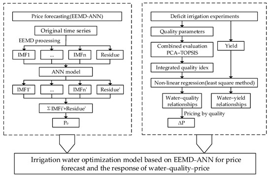
Figure 1.
The framework of this study.
3. Case Study
Tomato is the second largest vegetable crop in the world, and China is the country with the largest tomato planting area and the largest total production in the world [24]. With the development of economy and society and the improvement of living standards, consumers’ demand for quantity in tomato is saturated, while the demand for quality is increasing. Many studies have shown that deficit irrigation can improve the quality of tomato [39,40], but it is accompanied by a decrease in tomato yield and fruit size [41,42]. How to balance the contradictory relationship between tomato yield and fruit quality to maximize planting efficiency is a realistic problem that needs to be solved. Therefore, based on the previous experimental research, this paper established a tomato irrigation system optimization model that considered the water-yield-quality-benefit response relationship.
3.1. Data Collection
3.1.1. Field Experimental Data Collection
The observation data from four consecutive years of deficit irrigation experiments, including evapotranspiration, yield, and quality were collected from Chen et al. [8,12]. The four-year experiments aimed to determine the effects of deficit irrigation on the yield and quality of fresh-consumption greenhouse tomato. Experiments were conducted in the solar greenhouse at the Wuwei Experimental Station of Crop Water Use, Ministry of Agriculture, P.R. China which is located in Wuwei, Gansu province of northwest China (latitude 37°52’N, longitude 102°51’E, altitude 1581 m) [8], from winter 2008 to spring 2009 (2008–2009 season), from winter 2009 to spring 2010 (2009–2010 season), from spring to summer 2011 (2011 season), and from winter 2012 to spring 2013 (2012–2013 season). More details of the construction of solar greenhouses were described by Qiu et al. [43].
A growing season of tomato is usually divided into three stages: Vegetative (Stage I), flowering and fruit development (Stage II), and fruit ripening (Stage III). The crop evapotranspiration (ETc) and actual crop evapotranspiration (ETa) were obtained by the field water balance principle. The design, agronomy, and other details of the 2008/2009 and 2009/2010 experiments are reported in 2013 [8] and those of the 2011 and 2012/2013 experiments are reported in 2014 [12]. The ETa and yield for different irrigation treatments are shown in Table 1.

Table 1.
Actual crop evapotranspiration (ETa) and yield for different irrigation treatments in four growing seasons [12].
Consider seven individual indicators of tomato quality, namely: Total soluble solids content (TSS), reducing sugar (RS), organic acids content (OA), sugar/acid content ratio (SAR), vitamin C (VC), fruit firmness (Fn), and color index (CI). Among them, CI characterizes the appearance quality; TSS, RS, OA, and SAR characterize the taste quality; VC characterizes the nutritional quality; and Fn characterizes the storage quality of tomato. The specific quality parameters are shown in Table 2.
Table 2.
Tomato quality parameters for different irrigation treatments in four growing seasons [12] (TSS, total soluble solids; RS, reducing sugars; OA, organic acids; SAR, sugar/acid content ratio; VC, vitamin C; Fn, fruit firmness; CI, color index).
3.1.2. Other Data
The monthly price of tomato from 2009 to 2018 is obtained from the government website http://cif.mofcom.gov.cn/cif/html/dataCenter/index.html?jgnfcprd. The water-price data are collected from local policy surveys and the soil moisture content is collected from Chen [24], which are shown in Table 3.
Table 3.
Other data.
3.2. Irrigation Water Optimization Model
The optimization model of tomato irrigation schedule is established, aiming at the maximum net benefit of greenhouse tomato. The model optimizes the water consumption for each growth stage based on (1) the EEMD-ANN method for price forecasting, (2) the water–yield model at various growth stages, (3) the water–quality–price response relationship, and (4) the water balance principle. The water–yield–quality–benefit optimization model (WYQ) is shown as:
3.2.1. Objective Function
In this study, we selected the tomato under full irrigation treatment as a reference product; is the basic price of greenhouse tomato, which is forecasted by EEMD-ANN method, i.e., ; is the relative quality scores under full irrigation treatment; is the largest relative quality scores; and is the price range between the best quality and the tomato quality under full irrigation.
3.2.2. Constraints
(1) Soil moisture content constraint
where is the soil moisture content at the i-th growth stage (cm3/cm3); is the lower limit of volumetric water content, taken as the coefficient of wilting (cm3/cm3); and is the soil water holding capacity (cm3/cm3).
The amount of water that the planned wet layer of the soil can use for crops is
where is the effective water quantity available for the wet layer at the i-th growth stage (mm) and is the planned wet layer depth at the i-th growth stage.
Also, by the field soil water balance formula
where is the deep leakage of the i-th stage (mm); is the effective rainfall of the i-th stage (mm); and CK is the amount of groundwater recharge (mm).
There are some case-specific assumptions for greenhouse tomatoes: The effective rainfall is equal to 0 in the solar greenhouse and the deep leakage , and groundwater recharge CK are equal to 0. Equation (28) can be converted to
According to Equations (27) and (29), Equation (26) can be transformed to
where is the initial average soil volumetric moisture content of the planned wet layer.
(2) Crop water requirement constraint
In this study, the relative water deficit () during deficit irrigation experiments was controlled within 0.5, so the applicable range of the water-–yield and water–fruit quality are . After this range is exceeded, the models are not suitable.
4. Results and Discussion
4.1. The Results of Basic Price Forecasting by EEMD-ANN
For the EEMD model, the amplitude of white noise is set to 0.2 times the standard deviation of the sample data as suggested by Wu and Huang [18], and the realization number is set to 100. The original tomato price series from 2009 to 2018 are decomposed into a finite number of subseries. The decomposition results are shown in Figure 2. The original price series were decomposed into five independent IMF components and one residue component, respectively. The IMFs represent changing amplitudes, frequencies, and wavelengths. IMF 1 had the highest frequency, maximum amplitude, and shortest wavelength. IMFs 2–5 decreased in the amplitude and frequency and increased in wavelength. The residue slowly varied around the long-term average. The tomato price showed a growing trend in the past decade. IMF 2 showed a significant seasonal periodicity with maximum values in December–February and minimum in June–July. When forecasting the price of tomato on a monthly basis, it is necessary to consider not only its long-term price trend, but also its cyclical changes. Decomposition with EEMD can well separate its long-term trend from periodicity and avoid the problem of mode mixing.
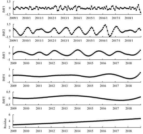
Figure 2.
Decomposition of tomato price series for the period of 2009–2018.
ANN was then used to forecast each subseries. In this study, the Levenberg–Marquardt methodology, which is more powerful than conventional gradient decent techniques [44], was used to adjust the weights and threshold values of neural network. The autoregressive order was 3. This case study was based on monthly price data for 2009–2018, and forecasts for 2019 were generated. First, BPNN was used to forecast each IMF and residue which were decomposed by EEMD. Figure 3 shows the forecasting results of each IMF and the residue. Then, the forecasting results of the IMFs and the residual from ANN were summed to obtain the forecasting price for 2009 to 2019. In addition, the ANN model was used to forecast the original price data without decomposition for comparison. Figure 4 shows the final forecasting results using the EEMD-ANN and ANN models. Finally, four evaluation criteria, including RMSE, MARE, R, and NSEC, were calculated. Table 4 presents the performance evaluation results of EEMD-ANN and ANN.
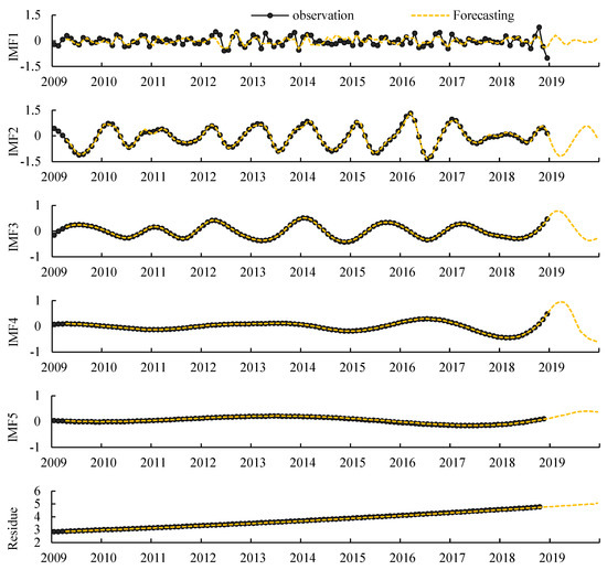
Figure 3.
The forecast results of each intrinsic mode functions (IMF) and the residue by the artificial neural network (ANN) model.
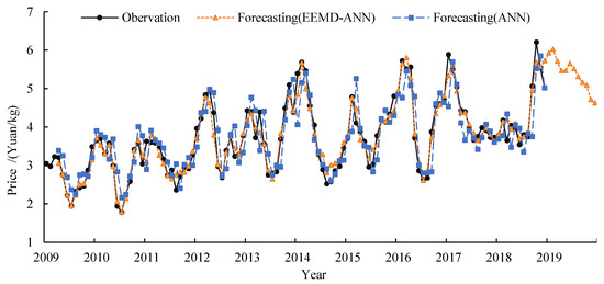
Figure 4.
The forecast results of tomato price using the EEMD-ANN (2009–2019) and ANN (2009–2018) models.
Table 4.
Forecasting performance indices of the EEMD-ANN and ANN models.
The closer the RMSE and MARE values are to 0, and the R and NSEC values are to 1, the better the performance of the forecast model would be. As shown in Table 5, the RMSE and MARE values of EEMD-ANN model were smaller than ANN, and the R and NSEC values were larger. Obviously, forecasting based on time-series decomposition is better than direct prediction without decomposing. Therefore, we can conclude that EEMD-ANN is a more useful method to forecast the tomato basic price.
Table 5.
Component score coefficient matrix after factor rotation and contribution rate.
4.2. The Solutions of FA-TOPSIS
Before performing factor analysis, a correlation analysis of the original variables was required. The F-value of the Bartlett spherical test was equal to 0.000, indicating that the data are from the population of a normal distribution. The Kaiser–Meyer–Olkin test value was 0.805, so it is suitable for factor analysis. Factor analysis of the tomato quality data in Table 5 was performed using SPSS statistical software 21.0 (IBM, New York, NY, USA). In this paper, the principal component method was used to extract three common factors. The factor load matrix, contribution rate, and cumulative contribution rate after the varimax rotation are shown in Table 5. The factor score and comprehensive index are shown in Table 6.
Table 6.
Tomato comprehensive quality scores for different irrigation treatments by factor analysis (FA), technique for order of preference by similarity to ideal solution (TOPSIS), and FA-TOPSIS methods.
The cumulative contribution rate of the first three common factors reached 95.301%. After extracting three factors, they reflect most of the information of the original variables. Factors 1 and 2, which explained 67.878% of the total variance Table 5), have strong positive loadings on TSS, RS, OA, and SAR. TSS, RS, OA, and SAR were the test indicators. Factor 3 explained 27.423% of the total variance, which had positive loadings on VC, Fn, CI.
In the TOPSIS method, the weights of quality indicators TSS, RS, OA, SAR, VC, Fn, and CI were 0.130, 0.130, 0.090, 0.190, 0.180, 0.120, and 0.160, respectively [24]. The comprehensive quality value of the greenhouse tomato under the TOPSIS method was calculated from Equations (10)–(15), and the results are shown in Table 6.
The weighted-average method based on Equation (16) was used to calculate the integrated evaluation score, in which the weights of the FA and TOPSIS methods were the same (i.e., ). The final results of the integrated evaluation are also shown in Table 6. From Table 6, we can see that, for the same growing season, the resulted rankings from FA, TOPSIS, and the combined approach were the same under different irrigation treatments.
4.3. Non-Linear Regression Results
The model parameters for each water–yield or water–fruit quality model were estimated using field observed data from 2008–2009, 2009–2010, and 2011 [12]. The model parameters were estimated using the least squares method. Subsequently, the calibrated model was validated using the 2012–2013 data.
4.3.1. Water–Yield Relationships
The actual crop evapotranspiration () for various growth stages in four growing seasons is given in Table 1. Table 7 presents the tomato-yield water-deficit sensitivity indexes (///) at various growth stages for the four water–yield models including the Jensen, Stewart, Blank, and Rao models. The values of the coefficient of determination () during simulation and verification are also presented in the table. From Table 7, we can see that for the four models, the values were all greater than 0.7, showing a good model performance. The Jenson, Stewart, Blank, and Rao water–yield models had positive water-deficit sensitivities at all stages of growth, with Stage III being the largest, Stage II being the second, and Stage I being the smallest. That is, tomato yield was most sensitive during fruit ripening-stage water deficit, followed by flowering and fruiting, and it was the least sensitive during the vegetative stage. All four water–yield quality models had positive sensitive indexes, indicating that the fruit yield increased with the increase of . Among the four models, Jensen model had the highest comprehensive R2 value. Therefore, the Jensen model was selected to simulate the relationship between water consumption and yield of greenhouse tomatoes.
Table 7.
The water deficit sensitivity indexes of tomato yield and the .
The water–yield model is as follows:
4.3.2. Water–Fruit Quality Relationships
The water-comprehensive quality model was fitted based on the evapotranspiration (Table 2) and the integrated evaluation of comprehensive evaluation value (Table 6) of irrigation treatments. Table 8 shows the tomato comprehensive quality water deficit sensitivity indexes (//) at various growth stages for three water–fruit quality models, including the multiplicative, additive, and exponential models, and the R2 during simulation and verification. Among three models, the additive model had the highest R2 value and performed better than the other models. Therefore, the additive model was chosen to simulate the relationship between water consumption and comprehensive quality of greenhouse tomatoes.
Table 8.
The water deficit sensitivity indexes of tomato comprehensive quality and the .
The water–fruit quality model (additive model) is as follows:
From the experiments results and Equation (33), we can find that tomato quality was most sensitive to Stage III, followed by Stage I and Stage II. Furthermore, the fruit quality of greenhouse tomato increased with the decrease of , which is opposite to the yield. When fully irrigated, the overall quality of the tomato was lowest. The reduction of tomato yield under deficit irrigation was accompanied by the improvement of fruit quality, indicating the contradictory relationship between yield and fruit quality.
4.4. Optimal Results and Discussion
4.4.1. Optimization MODEL
The solution of the water–yield model and the water–fruit quality model were brought into the optimization model WYQ. The reduced expression is as follows:
Regardless of the water–quality–price response, the water–yield–benefit optimization (WY) model was established at the same time for comparison with the WYQ model. The WY model is shown as follows:
Lingo was used to solve the WYQ model and the WY model. In order to further investigate the relationship between different socioeconomic conditions and optimal irrigation schemes, six scenarios were examined under three basic forecasted prices (maximum, minimum, and mean) and two price ranges between best and worst quality of tomato ().
4.4.2. Optimal Solution of WYQ
Figure 5 represents the optimal actual crop evapotranspiration and net benefits under different socioeconomic conditions (different and different ) of the WYQ model. Among them, = 6.03, 5.39, and 4.62 represent the highest, average, and lowest monthly average price of tomato in 2019, respectively, which were forecasted by EEMD-ANN method; = 0.5 and 1.0 were set to indicate that the same quality difference would result in the different price differences, which is caused by market demand conditions.
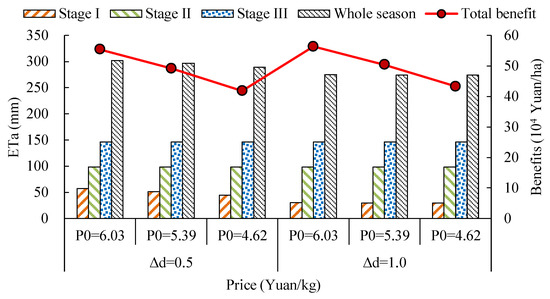
Figure 5.
Actual crop evapotranspiration (ETa) and total benefits under different and of the water–yield–quality–benefit optimization (WYQ) model.
According to the results described in Section 4.3, as the amount of water increased, the greenhouse tomato yield would increase and the fruit quality would decrease. The WYQ model can energize the contradiction between tomato yield and quality and provide the optimal under different market conditions. It can be seen from Figure 5 that among the six scenarios, the water requirement in the whole growth period increased with the increase of , and decreased with the increase of . Specifically, the WYQ model tended to preferentially meet the crop water requirement of the second and third growth stages of tomato, namely , . In contrast, , i.e., water requirement of crops in the first growth stage of tomato, was strongly affected by and . For the same , as the price of tomato increased, increased. Taking = 0.5 Yuan/kg as an example, when changed from 4.62, 5.39, to 6.03 Yuan/kg, increased to 44.6, 51.5, and 57.2 mm, respectively. For the same , with the increase of , decreased. When changed from 0.5 to 1 Yuan/kg, was reduced from 57.2 to 30.2 mm, from 51.5 to 29.2 mm, and from 44.6 to 29.2 mm, when was equal to 6.03, 5.39, and 4.62 Yuan/kg, respectively. This suggests that Stage II (flowering and fruit development stage) and Stage III (fruit ripening stage) are more important than Stage I (vegetative stage) in irrigation management, thus the water requirements at these two stages should be prioritized.
For the optimal irrigation targets, Figure 5 shows that the increasing basic price of greenhouse tomato () had a positive effect on net benefits. Taking = 0.5 Yuan/kg as an example, when changed from 4.62, 5.39, to 6.03 Yuan/kg, the net benefits increased to 41.8, 49.2, and 55.4 × 10⁴ Yuan/ha, respectively. At this point, the difference between the highest and lowest net benefits were 13.56 × 10⁴ Yuan/ha, accounting for 25% of the highest. Obviously, the basic price has a direct and important impact on farmers’ income from planting tomato. Therefore, the use of more accurate price forecasting methods, such as EEMD-ANN, can provide effective advice for farmers to arrange greenhouse-tomato planting scale and planting date, thereby increasing farmers’ economic income.
Similarly, the net benefits increased when increased and was fixed. When compared with , the net benefits per plant area increased by 1.8%, 2.5%, and 3.4% at = 6.03, 5.39, and 4.62 Yuan/kg, respectively. The results indicate that increasing the value of means that the market price is more sensitive to tomato quality, which will result in more economic benefits.
From the above results, an interesting phenomenon can be obtained: When the market price is more sensitive to fruit quality, the WYQ model tends to reduce the crop water demand while the benefit increases. Taking = 5.39 as an example, when increased from 0.5 to 1.0, changed from 51.5 to 29.2 mm while the benefit changed from 49.17 to 50.39 × 10⁴ Yuan/ha. This is because characterizes the price difference due to changes in tomato quality. When is larger, it indicates that the market price difference caused by the same quality change of tomato is larger. There was a negative correlation between the water requirement of tomato and the comprehensive quality index. Therefore, when the price of the tomato market is more affected by the quality, the WYQ model tends to reduce the water distribution to obtain better quality and thus obtain higher returns. Less water brings higher benefits, which suggests that it is necessary to consider the water–quality–benefit relationship at this time. This also provides irrigation advice to farmers: Full irrigation does not bring the highest benefits when the market price is more sensitive to tomato quality. Local farmers should appropriately reduce the amount of irrigation especially in Stage I, in order to improve the quality of tomatoes and thus obtain higher economic benefits at this time.
4.4.3. Discussion
The WY model was established and solved for comparison. Table 9 presents the obtained results from the WY and WYQ ( and ) models with the highest, lowest, and average price. The WY model does not address the water–fruit quality relationship. Since the effect of water quantity on yield is positively correlated, the optimal crop water requirement for each growth stage is fully irrigated, i.e., , , . From Table 9, we can see that the net benefits per unit area is lower and the optimal irrigation water in the whole season is higher in the WY model than the WYQ model. Therefore, the water-use efficiency (benefits/irrigation water) of the WYQ model is greater than the WY model. For example, the water-use efficiency of the WYQ model is increased by 15.4% and 18.2% compared with the WY model under the scenario of . As increases, the differences in net benefits and water-use efficiency between the two models increase. When is larger, the price of better-quality tomatoes is significantly higher. At this time, if the greenhouse tomato is fully irrigated using the results of the WY model, the quality of the harvested tomato is poor. This is obviously not a good decision, not only because of the more water consumed, but also because the lower quality makes the sale price lower and the net income does not increase. In fact, the WY model is included in the WYQ model. When , the WYQ model is equivalent to the WY model. Therefore, the WYQ model that considers the economic mechanism of market price changes with fruit quality is more useful and is able to better reflect the reality.
Table 9.
Comparison of optimal results from the water–yield–benefit optimization (WY) and WYQ ( and ) models.
The WYQ model established in this study can provide more scientific and effective decision-making support to the cultivation and irrigation of greenhouse tomatoes. On one hand, by forecasting the monthly price of greenhouse tomatoes, the model can help farmers analyze the future market and provide decision-making reference to arrange greenhouse-tomato planting time and planting scale. On the other hand, the WYQ model balances the contradiction between higher yields and better quality by controlling irrigation. When the market demand for tomato quality is higher (larger , such as scenario ), the amount of water in Stage I is reduced to obtain higher quality. Therefore, the WYQ model can provide farmers with the best irrigation advice under different market conditions to obtain the highest economic benefits.
5. Conclusions
An optimal irrigation scheduling model was established considering the water–yield–quality–benefit relationship and is applied to the irrigation management of solar greenhouse tomatoes. In this model, EEMD-ANN, FA-TOPSIS, and regression analysis were incorporated into a general optimization model. Among them, the EEMD-ANN method is used to decompose the original tomato price time series into six subseries for price forecasting. FA-TOPSIS, as an integrated evaluation method, is used to comprehensively evaluate seven quality parameters of tomato; regression analysis is used to simulate water–yield and water–fruit quality relationships of tomato; six scenarios with different market conditions were considered in the case study. The following conclusions can be drawn from this study:
- (1)
- For the monthly forecast of tomato price, the EEMD-ANN model can significantly improve forecast accuracy compared with ANN method.
- (2)
- In the WYQ model, it can be found that Stages II and III of tomato are more important than Stage I, and meeting their water requirement should be a priority.
- (3)
- Considering the economic mechanism of market price changes with fruit quality, the irrigation scheduling optimization model can achieve the purposes of saving water resources, improving net benefit, increasing quality, and improving water-use efficiency.
The model presented in this paper can be used to optimize irrigation scheduling for other economic crops. In the actual situation, the harvest phase of greenhouse tomatoes generally lasts for a period of time. In this study, this was not taken into account by field experiment and data limitations. In addition, there are many uncertainties in the optimization of crop irrigations, including the farmer response to the market price and government regulation. In future research, the above issues need to be considered in improved models.
Author Contributions
Conceptualization: B.S. and P.G.; methodology: B.S.; data curation: B.S. and S.G.; writing–original draft preparation: B.S., S.G., and P.G.; writing–review and editing: Z.L. and P.G.; supervision: P.G. and Z.L.
Funding
This research was supported by the National Key Research and Development Plan (No. 2016YFC0400207), Chinese Universities Scientific Fund (No. 2018TC013).
Conflicts of Interest
The authors declare no conflict of interest.
References
- Li, M.; Fu, Q.; Singh, V.P.; Ma, M.; Liu, X. An intuitionistic fuzzy multi-objective non-linear programming model for sustainable irrigation water allocation under the combination of dry and wet conditions. J. Hydrol. 2017, 555, 80–94. [Google Scholar] [CrossRef]
- Zhang, C.; Fan, Z.; Guo, S.; Xiao, L.; Ping, G. Inexact nonlinear improved fuzzy chance-constrained programming model for irrigation water management under uncertainty. J. Hydrol. 2018, 556, 397–408. [Google Scholar] [CrossRef]
- Behboudian, M.H.; Lawes, G.S.; Griffiths, K.M. The influence of water deficit on water relations, photosynthesis and fruit growth in Asian pear (Pyrus serotina Rehd.). Sci. Horticult. 1994, 60, 89–99. [Google Scholar] [CrossRef]
- Mills, T.M.; Behboudian, M.H.; Clothier, B.E. Water Relations, Growth, and the Composition of ‘Braeburn’ Apple Fruit under Deficit Irrigation. J. Am. Soc. Horticult. Sci. 1996, 121, 286–291. [Google Scholar] [CrossRef]
- Pomper, K.W.; Breen, P.J. Expansion and Osmotic Adjustment of Strawberry Fruit during Water Stress. J. Am. Soc. Horticult. Sci. 1997, 122, 183–189. [Google Scholar] [CrossRef]
- Shellie, K.C. Vine and berry response of Merlot (vitis vinifera L.) to differential water stress. Am. J. Enol. Viticult. 2006, 57, 514–518. [Google Scholar]
- Marouelli, W.A.; Silva, W.L.C. Water tension thresholds for processing tomatoes under drip irrigation in Central Brazil. Irrig. Sci. 2007, 25, 411–418. [Google Scholar] [CrossRef]
- Chen, J.; Kang, S.; Du, T.; Qiu, R.; Guo, P.; Chen, R. Quantitative response of greenhouse tomato yield and quality to water deficit at different growth stages. Agric. Water Manag. 2013, 129, 152–162. [Google Scholar] [CrossRef]
- Sensoy, S.; Ertek, A.; Gedik, I.; Kucukyumuk, C. Irrigation frequency and amount affect yield and quality of field-grown melon (Cucumis melo L.). Agric. Water Manag. 2007, 88, 269–274. [Google Scholar] [CrossRef]
- Leib, B.G.; Caspari, H.W.; Redulla, C.A.; Andrews, P.K.; Jabro, J.J. Partial rootzone drying and deficit irrigation of ‘Fuji’ apples in a semi-arid climate. Irrig. Sci. 2006, 24, 85–99. [Google Scholar]
- Du, T.; Kang, S. Efficient water-saving irrigation theory based on the response of water and fruit quality for improving quality of economic crops. J. Hydr. Eng. 2011, 42, 245–252. [Google Scholar]
- Chen, J.; Kang, S.; Du, T.; Guo, P.; Qiu, R.; Chen, R.; Gu, F. Modeling relations of tomato yield and fruit quality with water deficit at different growth stages under greenhouse condition. Agric. Water Manag. 2014, 146, 131–148. [Google Scholar] [CrossRef]
- Zhang, W.; Chen, H.; Wang, M. A Forecast Model of Agricultural and Livestock Products Price. Appl. Mech. Mater. 2010, 20–23, 1109–1114. [Google Scholar] [CrossRef]
- Chenglong, Z.; Engel, B.A.; Ping, G. An Interval-based Fuzzy Chance-constrained Irrigation Water Allocation model with double-sided fuzziness. Agric. Water Manag. 2018, 210, 22–31. [Google Scholar]
- Pastori, M.; Udias, A.; Bouraoui, F.; Bidoglio, G. A Multi-Objective Approach to Evaluate the Economic and Environmental Impacts of Alternative Water and Nutrient Management Strategies in Africa. J. Environ. Inform. 2015, 29, 16–28. [Google Scholar] [CrossRef]
- Wang, W.C.; Chau, K.W.; Qiu, L.; Chen, Y.B. Improving forecasting accuracy of medium and long-term runoff using artificial neural network based on EEMD decomposition. Environ. Res. 2015, 139, 46–54. [Google Scholar] [CrossRef]
- Tan, Q.-F.; Lei, X.-H.; Wang, X.; Wang, H.; Wen, X.; Ji, Y.; Kang, A.-Q. An adaptive middle and long-term runoff forecast model using EEMD-ANN hybrid approach. J. Hydrol. 2018, 567, 767–780. [Google Scholar] [CrossRef]
- Wu, Z.; Huang, N.E. Ensemble Empirical Mode Decomposition: A Noise-Assisted Data Analysis Method. Adv. Adapt. Data Anal. 2009, 1, 1–41. [Google Scholar] [CrossRef]
- Huang, N.E.; Zheng, S.; Long, S.R.; Wu, M.C.; Shih, H.H.; Zheng, Q.; Yen, N.C.; Chi, C.T.; Liu, H.H. The empirical mode decomposition and the Hilbert spectrum for nonlinear and non-stationary time series analysis. Proc. Math. Phys. Eng. Sci. 1998, 454, 903–995. [Google Scholar] [CrossRef]
- Huang, N.E.; Wu, Z. A review on Hilbert-Huang transform: Method and its applications to geophysical studies. Rev. Geophys. 2008, 46, L13705. [Google Scholar] [CrossRef]
- Haykin, S. Neural Networks: A Comprehensive Foundation, 2nd ed.; Prentice Hall PTR: Upper Saddle River, NJ, USA, 1998. [Google Scholar]
- Rojas, R. Neural Networks: A Systematic Introduction; Springer Science & Business Media: Berlin, Germany, 1996. [Google Scholar]
- Chen, J.S.; Chen, W.G.; Li, J.; Sun, P. A generalized model for wind turbine faulty condition detection using combination prediction approach and information entropy. J. Environ. Inform. 2018, 32, 14–24. [Google Scholar] [CrossRef]
- Chen, J. Modeling Fruit Growth and Sugar Accumulation and Optimizing Irrigation Scheduling for Improving Water Use Efficiency and Fruit Quality of Tomato. Ph.D. Thesis, China Agricultural University, Beijing, China, 2016. [Google Scholar]
- Wang, F.; Du, T.; Qiu, R. Deficit irrigation scheduling of greenhouse tomato based on quality principle component analysis. Trans. CSAE 2011, 27, 75–80. [Google Scholar]
- Tong, L.; Wang, C.; Chen, H. Optimization of multiple responses using principal component analysis and technique for order preference by similarity to ideal solution. Int. J. Adv. Manuf. Technol. 2005, 27, 407–414. [Google Scholar] [CrossRef]
- Gumus, A.T. Evaluation of hazardous waste transportation firms by using a two step fuzzy-AHP and TOPSIS methodology. Expert Syst. Appl. 2009, 36, 4067–4074. [Google Scholar] [CrossRef]
- Jia, W.; He, J. Application of Principal Component Analysis and Factor Analysis in Evaluating Regional Economic Development Level. Modern Manag. Sci. 2007, 19–21. [Google Scholar] [CrossRef]
- Liu, C.-W.; Lin, K.-H.; Kuo, Y.-M. Application of factor analysis in the assessment of groundwater quality in a blackfoot disease area in Taiwan. Sci. Total Environ. 2003, 313, 77–89. [Google Scholar] [CrossRef]
- Kaiser, H.F. The varimax criterion for analytic rotation in factor analysis. Psychometrika 1958, 23, 187–200. [Google Scholar] [CrossRef]
- Hwang, C.-L.; Yoon, K. Multiple Attribute Decision Making, Methods and Applications. Lecture Notes in Economics and Mathematical Systems; Springer: New York, NY, USA, 1981. [Google Scholar]
- Tzeng, G.-H.; Huang, J.-J. Multiple Attribute Decision Making: Methods and Applications; Chapman and Hall/CRC: Boca Raton, FL, USA, 2011. [Google Scholar]
- Jensen, M.E. Water consumption by agricultural plants. In Plant Water Consumption and Response. Water Deficits and Plant Growth, 1st ed.; Kozlowski, T.T., Ed.; Academic Press: New York, NY, USA, 1968; Volume 2, pp. 1–22. [Google Scholar]
- Stewart, J.I.; Misra, R.D.; Puritt, W.O.; Hagan, R.M. Irrigating Corn and Grain Sorphum with a Deficient Water Supply. Trans. ASAE 1975, 18, 260–270. [Google Scholar] [CrossRef]
- Blank, H.G. Optimal Irrigation Decisions with Limited Water, unpublished. Ph.D. Thesis, Colorado State University, Fort Collins, CO, USA, 1975. [Google Scholar]
- Rao, N.H.; Sarma, P.B.S.; Chander, S. A simple dated water-production function for use in irrigated agriculture. Agric. Water Manag. 1988, 13, 25–32. [Google Scholar] [CrossRef]
- Zhao, M.; Li, Y. Discussion on the specific method of quality. Price Theory Pract. 1991, 6, 31–33. [Google Scholar]
- Wang, F. Response of Greenhouse Tomato Yield and Quality to Water Stress and the Irrigation Index for Water Saving & Fruit Quality Improving. Ph.D. Thesis, China Agricultural University, Beijing, China, 2016. [Google Scholar]
- Favati, F.; Lovelli, S.; Galgano, F.; Miccolis, V.; Di Tommaso, T.; Candido, V. Processing tomato quality as affected by irrigation scheduling. Sci. Horticult. 2009, 122, 562–571. [Google Scholar] [CrossRef]
- Patanè, C.; Cosentino, S.L. Effects of soil water deficit on yield and quality of processing tomato under a Mediterranean climate. Agric. Water Manag. 2010, 97, 131–138. [Google Scholar] [CrossRef]
- Machado, R.M.; Maria do Rosàrio, G.O. Tomato root distribution, yield and fruit quality under different subsurface drip irrigation regimes and depths. Irrig. Sci. 2005, 24, 15–24. [Google Scholar] [CrossRef]
- Zheng, J.; Huang, G.; Jia, D.; Wang, J.; Mota, M.; Pereira, L.S.; Huang, Q.; Xu, X.; Liu, H. Responses of drip irrigated tomato (Solanum lycopersicum L.) yield, quality and water productivity to various soil matric potential thresholds in an arid region of Northwest China. Agric. Water Manag. 2013, 129, 181–193. [Google Scholar] [CrossRef]
- Qiu, R.; Kang, S.; Li, F.; Du, T.; Tong, L.; Wang, F.; Chen, R.; Liu, J.; Li, S. Energy partitioning and evapotranspiration of hot pepper grown in greenhouse with furrow and drip irrigation methods. Sci. Horticult. 2011, 129, 790–797. [Google Scholar] [CrossRef]
- Hagan, M.T.; Menhaj, M.B. Training feedforward networks with the Marquardt algorithm. IEEE Trans. Neural Netw. 1994, 5, 989–993. [Google Scholar] [CrossRef] [PubMed]


© 2019 by the authors. Licensee MDPI, Basel, Switzerland. This article is an open access article distributed under the terms and conditions of the Creative Commons Attribution (CC BY) license (http://creativecommons.org/licenses/by/4.0/).