Article

Spatio-Temporal Variation in Mountainous Landscape Changes: A Case Study of Shizhu County

1
College of Horticulture and Landscape Architecture, Southwest University, Chongqing 400715, China
2
College of Geography and Tourism, Chongqing Normal University, 37 Daxuechengzhong Road, Chongqing 401331, China
3
Chongqing Key Laboratory of GIS Application, 37 Daxuechengzhong Road, Chongqing 401331, China
4
Institute of Eco-Environment Remote Sensing in Three Gorges Reservoir Region, Chongqing Normal University, 37 Daxuechengzhong Road, Chongqing 401331, China
5
Office of Academic Affairs, Chongqing Normal University, Chongqing 401331, China
*
Author to whom correspondence should be addressed.
Sustainability 2019, 11(7), 2131; https://doi.org/10.3390/su11072131
Submission received: 29 December 2018 / Revised: 27 March 2019 / Accepted: 8 April 2019 / Published: 10 April 2019
(This article belongs to the Section Sustainable Urban and Rural Development)

Abstract

:
The study of dynamic changes and spatial variation of landscape patterns is important to deeply understand the relationship between human activities and the natural environment. We selected a typical mountain area, Shizhu County, as the study area and analyzed the landscape’s dynamic changes and spatial variation in that area from 2000–2015. The results showed that cropland and forestland were the dominant landscape types in the study area. Cropland and grassland areas decreased, being mainly converted to forestland. Forestland and built-up land areas were increasing; the increase in built-up land was mainly due to the invasion into cropland areas, and the increase in forestland was mainly due to the conversion of cropland and grassland. Water bodies were affected by factors such as water storage in the Three Gorges Reservoir, and their area continued to increase. The change in landscape was most dramatic from 2005–2010, mainly due to the rapid increase in the areas of built-up land and water bodies and the rapid decrease in grassland area. There were apparent spatial variations in landscape distribution, patterns, and dynamic changes. Although water bodies were mainly distributed in the relatively gentle slope areas with an elevation of less than 200 m and a slope of 0°–6°, other landscapes were concentrated at an elevation higher than 500 m, a slope of 15°–35°, with a westerly or northwesterly aspect. These areas also had the most drastic landscape changes. At the type-level and the landscape-level, landscape indices showed greater variation with elevation and slope than with aspect. Finally, the variations with elevation, slope, and aspect differed among different landscape types.

1. Introduction

Land is the site of various social and economic activities. The breadth, depth, and changes in land-use will directly affect the evolution of the environmental system. A landscape pattern is a spatial configuration of different landscape elements with dynamics through time; in other words, a landscape pattern results from the interaction of landscape structure and landscape ecological processes at different scales [1]. A landscape index contains concentrated landscape pattern information; therefore, these indices are widely used in the analysis of landscape patterns [2]. Landscape patterns, represented by the mosaic patches of different land-use types, reflect the land’s ecological evolution [3]. Exploring the characteristics and evolution of landscape patterns is an important way to understand the relationship between human activities and the natural environment. It is an important breach point to solve the current human–land conflict, promote human–land harmony, and achieve sustainable development [4,5,6]. At present, landscape patterns have become one of the key areas of regional and global environmental research and have become the frontier and focus of climate change research [7,8,9,10]. In 2005, the Global Land Project (GLP) was launched, with the “human–land coupled system” as the research goal, focusing on the driving mechanism and eco-environmental consequences of land-use changes [11]. The project pays special attention to the study of urban landscapes with the most frequent human activities at different geographic scales [12,13,14] and the study of the evolution of landscape patterns in typical regions and popular areas, covering watersheds [15,16,17,18], lakes [19,20,21], wetlands [22], plains [23], deltas [24], dams [25], and basins [26]. In addition, some scholars have studied the landscape of mountainous areas, such as the evolution of the land-use/-cover landscape patterns in karst mountains [27,28,29]. In addition, Li et al. studied the coupling process of land-use and landscape-pattern evolution in the mountain-dam system of Guizhou Province [30]. Zhang et al. studied land-use landscape pattern changes at a small scale in mountainous areas of Yujin Town, Qianwei County. They believed that the high degree of fragmentation in rural settlements is a common land-use problem in mountainous areas [31]. Furthermore, Chen et al. used a number of indices to explore the grain size effect of landscape patterns in the Three Gorges Reservoir area and its response to land-use/-cover change processes [32]. Taking the main urban area of Chongqing as an example, Jia et al. used the land-use dynamic index and reduction-strength index to analyze the dynamic changes of land-use landscape patterns in mountainous cities [33]. Their research showed that a “multi-center, cluster-type” urban landscape pattern was formed due to the barrier of mountains and rivers; however, with urbanization, this pattern tended to be weakened [33]. Wen et al. analyzed the land-use landscape pattern of different soil types in the hilly areas of central South China [34]. All the above studies enriched the literature in this field and facilitated the research progress of related fields and methods. However, the current research on landscape patterns is mostly based on landscape indices of two-dimensional information. There is still a lack of research on the spatial patterns and heterogeneity of the landscape and the effect of topographic factors [2,35,36]. Therefore, it is of great theoretical significance to carry out spatial heterogeneity studies of landscape changes in typical areas.
Shizhu County is a typical mountainous area, and it is a biologically diverse area in Chongqing. With the development of Western China, the rapid urbanization, and the water storage in the Three Gorges Reservoir, the landscape patterns of Shizhu County have undergone tremendous changes. The area’s ecological location and typical landform types add to the complexity and heterogeneity of the landscape evolution. Therefore, this paper uses Shizhu County, which has typical mountainous features in the hinterland of the Three Gorges Reservoir area, as the study area, to examine the spatio-temporal evolution of the landscape and its spatial heterogeneity. This will have practical value for promoting the proper use of regional land resources and sustainable development of the environment.

2. Materials and Methods

2.1. Study Area

Shizhu County is located on the southern bank of the southeastern Yangtze River in Chongqing, the hinterland of the Three Gorges Reservoir area, with a northern latitude of 29°39’–30°32’ and eastern longitude of 107°59’–108°34’ (Figure 1). The study area was 98.30 km long from north to south and 56.20 km wide from east to west, with a total area of 3012.51 km2, including 33 townships. At the end of 2017, the residential population was 379,100, of which the agricultural population was 181,100. Shizhu County has 28 minority ethnic groups. In 2017, the county’s Gross Regional Production (GRP) was 16.2 billion yuan, and the ratio of primary, secondary, and tertiary industry was 15.4:51.1:33.5. Fangdou Mountain and Qiyao Mountain are nearly parallel and run through the whole county, forming the geomorphological features of “two mountains and one valley.” The terrain is high in the southeast and low in the northwest, with an undulating decline. The elevation of the area is 119–1934.10 m, with mainly mid- and low-mountains, as well as plains and hills. It has a representative southwestern mountainous landform. This area falls in the subtropical humid monsoon climate zone with an average annual temperature of 16.5°C and an average annual precipitation of 1103.0 mm. The soil is mainly composed of yellow soil, yellow brown soil, purple soil, and paddy soil. The land-use/-cover landscape is dominated by forestland, and forest coverage exceeds 60%.

2.2. Data Sources and Processing

The data used in the study mainly included four years of land-use maps in the study area (2000, 2005, 2010, and 2015). Other data included a topographical map (1:10,000) and administrative maps of the study area from Shizhu Land Bureau, Digital Elevation Model (DEM) data (with a resolution of 25 m) from geospatial data clouds, and data derived from the above data, such as slopes and aspects. Land-use datasets were interpreted from Landsat images using visual digitalization. The images were obtained from Geospatial Data Cloud, Computer Network Information Centre, and Chinese Academy of Sciences (Table 1). In order to ensure the classification precision, we adopted images with cloud cover less than 5% and clear interpretation keys (hue, color, texture, shape, etc.). It should be noted that there was only one available image in 2005, and the cloud cover was large. Therefore, an image of roughly the same period of time in 2006 was selected to restore the images of cloud regions instead. First, we selected 30 control points for the 2015 image by using the 1:10,000 topographic map. A polynomial correction model was used for geometric correction of the 2015 image. Then, the geometric correction of the remaining images was carried out based on the geometric corrected images in 2015. Correction errors were controlled within 0.5 pixels. With the help of the FLAASH module in ENVI, the atmospheric correction of all images was made by using the MODTRAN model. Finally, the images of the study area were obtained by using the boundary vector map to cut the corrected images. The land-use types in the study area were divided into six categories: cropland, forestland, grassland, water bodies, built-up land, and unused land (Figure 2) by using visual digitalization. The image of 2000 was visually interpreted by reference to the historical land-use/-cover data in the study area, and then based on the classification results of 2000, the land-use/-cover data of 2005, 2010, and 2015 were obtained by comparing the images of 2005, 2010, and 2015 with 2000. Field verification and the high spatial resolution remote sensing image verification method were used to evaluate the classification accuracy. The field verification information comes from the field sampling data in the Geographical Conditions Census provided by Shizhu Land Bureau and the high spatial resolution remote sensing images mainly from Google Earth. Three hundred sample points (50 sample points for each land-use/-cover type) were selected to evaluate the land-use/-cover data accuracies. The overall accuracies of the datasets exceeded 85% (86.67%, 85.34%, 87.00%, 87.33% for 2000, 2005, 2010, 2015, respectively), and the kappa coefficients exceeded 0.8 (0.840, 0.823, 0.844, 0.848 for 2000, 2005, 2010, 2015, respectively). All data were uniformly converted into Albers equal-area projection for spatial operations. To simplify spatial operations, all data were converted to grid format with a grid cell size of 25 m × 25 m.

2.3. Analysis of Landscape Dynamics

The total area change of different land-use landscape types can reflect the extent and general trend of regional land-use/-cover landscape changes. This paper used both individual and composite land-use type dynamic indices (DIs) to analyze the dynamic changes of land-use/-cover landscape in the study area [37,38], in order to reflect the intensity of the changes in regional land-use/-cover landscape types.
• Individual land-use DI
The individual land-use DI was introduced into the spatial pattern analysis of landscape change, aiming to study the speed of change in an individual landscape type in Shizhu County. The equation is:
K s   =   U b U a U a   ×   1 T   ×   100 % ,
where Ks is the DI of an individual landscape type during the study period; Ua and Ub are the numbers of that landscape type at the beginning and at the end of the study period, respectively; and T is the length of the study period.
• Composite land-use DI
The composite land-use DI was used to represent the transfer and change between various landscape types in an area. The equation is:
R = i = 1 n | Δ U i j Δ U j i | 2 i = 1 n U i × 1 T × 100 % ,
where R is the composite land-use DI; ΔUi-j indicates the area of i landscape type converted to non-i landscape type; and ΔUj-i indicates the area of non-i landscape type converted to i landscape type. Ui indicates the area of i landscape type at the beginning of the study period; and T is the length of the study period.

2.4. Analysis of Landscape Pattern

Referring to the relevant literature [39,40,41,42] and considering the actual conditions of the study area, this paper selected three type-level landscape indices and five landscape-level landscape indices for analysis at different scales. The type-level indices reflect the structural features of different patch types in each landscape. This study adopted three relatively independent advantageous landscape indices—patch density (PD), largest patch index (LPI), and aggregation index (AI)—to study the landscape structural features in terms of basic structures, fragmentation, heterogeneity, and patch complexity. The landscape-level indices reflect the overall structural features of the landscape. According to the landscape features of the study area and the correlations between the landscape-level indices, we used the Shannon diversity index (SHDI), landscape contagion (CONTAG), PD, LPI, and AI to analyze the county’s pattern changes at the landscape level.

2.5. Analysis of Landscape Spatial Variation

The study area is a typical mountainous area, and the topographic factors have a significant impact on the change in the landscape pattern. To determine the spatial variation of the landscape pattern of the study area with various topographic factors, we used the spatial analysis function of GIS to divide the landscape into gradients according to different topographic factors and statistically analyzed the variation in the landscape along the terrain factor gradient. We analyzed the relationships between landscape and elevation, slope, and aspect, the three most important topographic factors. Based on the features of the study area, the classification of the elevation was <200 m, 200–300 m, 300–500 m, 500–800 m, and >800 m. The classification of the slope was <6°, 6–15°, 15–25°, 25–35°, and >35°. The classification of the aspect was as follows: gentle slope, easterly aspect, southeasterly aspect, southerly aspect, southwesterly aspect, westerly aspect, northwesterly aspect, northerly aspect, and northeasterly aspect.

3. Results

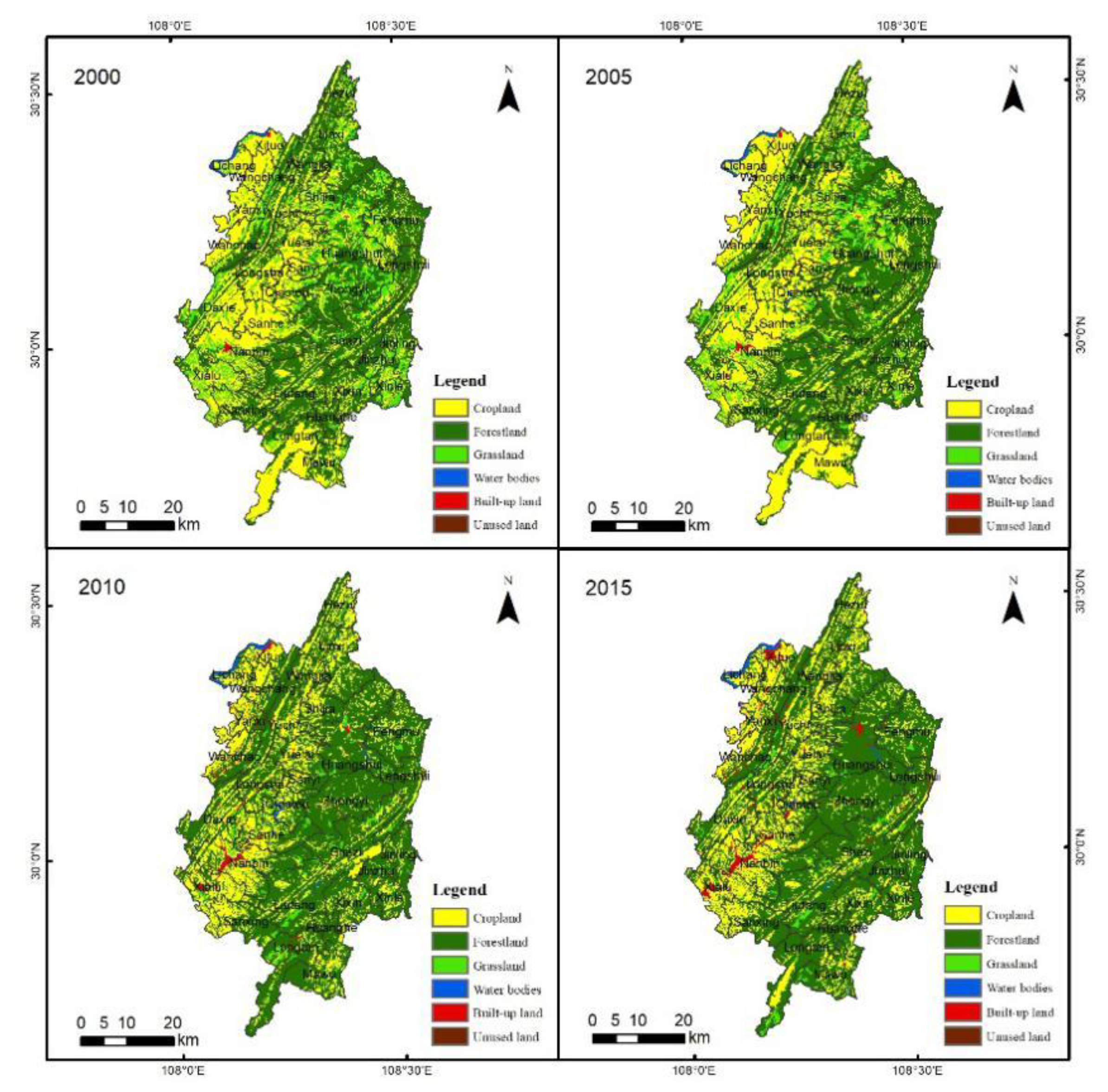
3.1. Dynamics of the Landscape and Their Spatial Variation

3.1.1. Characteristics of Landscape Dynamics

Cropland and forestland were the dominant landscape types in the study area. Cropland was mainly distributed in the northwestern, central, and southern parts of the study area. Forestland was concentrated in the northern, eastern, and southern areas. Conversely, grassland, water body, built-up land, and unused land accounted for a small proportion, scattered between cropland and forestland. Cropland and grassland showed an overall decreasing trend, and the respective area ratios decreased from 37.81% and 12.85%, respectively, in 2000 to 27.49% and 2.06%, respectively, in 2015. The two land-use types were mainly converted to forestland. Forestland and built-up land showed an increasing trend, and the respective area ratios increased rapidly from 48.72% and 0.16%, respectively, in 2000 to 67.41% and 1.85%, respectively, in 2015. The increase in built-up land was mainly due to the invasion into cropland, and the increase in forestland mainly came from the conversion of cropland and grassland. In addition, water bodies showed sustained growth. The area ratio increased from 0.43%–1.17% during the study period (Table 2). In terms of landscape change DI, landscape change was the most intensive during 2005–2010 (the composite DI was 17.06%), followed by 2000–2005 (the composite DI was 3.84%). The change was relatively gentle during 2010–2015 (the composite DI was 1.68%). In 2005–2010, the change was mainly due to the rapid increase in built-up land and water bodies and the rapid decrease in grassland; the DIs of these three land-use types were 69.45%, 10.3%, and −13.87%, respectively. From 2000–2005, the main characteristics were the relatively rapid increase in water bodies, built-up land, and unused land and the decrease in grassland (DIs were 14.89%, 9.82%, 8.42%, and −5.97%, respectively). Although the landscape change in 2010–2015 was relatively small, built-up land still increased while unused land and grassland decreased (Table 3).

3.1.2. Spatial Variation of Landscape Dynamics

1. Variation with elevation
Cropland was mainly distributed in areas above 500 m with an area ratio exceeding 85%. Forestland, grassland, and unused land were highly concentrated in areas above 800 m, with area ratios of 90%, 75%, and 70%, respectively. Water bodies were mainly distributed in areas below 200 m, with an area ratio of about 50%. In addition, approximately 30% and 15% of the water bodies were distributed in areas between 500 and 800 m and above 800 m, respectively. About 50% of the built-up land was distributed in areas between 500 and 800 m, and another 20% and 10% of the built-up land were distributed in areas above 800 m and from 200–300 m, respectively.
The areas with large composite DIs were mainly distributed in the areas above 800 m and between 500 and 800 m. The changes were the most intensive in the 2005–2010 period. Cropland showed a slow increasing trend at all elevation levels from 2000–2005, and the increase was slightly higher at the elevations of 500–800 m and 200–300 m than at other elevations. From 2005–2010 and 2010–2015, cropland decreased at all elevation ranges. The difference was that the decrease in cropland from 2005–2010 was larger than that in other periods. Except for the relatively small decrease at the elevation of 500–800 m, cropland decreased substantially at all other elevation ranges. However, from 2010–2015, except for the <200 m elevation range, where the cropland showed a large decrease, all other elevation ranges had small decreases in cropland. From 2000–2005, forestland showed a rapid increase in the <200-m areas (with a DI of 8.92%) and a slight decrease in the 500–800-m areas (with a DI of −1.84%). From 2005–2010, forestland increased rapidly at all elevation ranges, especially for the ranges of 200–300 m, <200 m, and 300–500 m. During the study period, grassland decreased, and the overall trend was a greater increase with decreasing elevation. However, during 2000–2005, the DI of grassland in areas of the >800-m range increased slightly, and during 2010–2015, the DI of grassland increased considerably in the range of 500–800 m. Water bodies with strong dynamics were mainly distributed in areas of 500–800 m, >800 m, and 300–500 m. The elevational variation patterns of built-up land showed that the areas below 300 m exhibited a strong increase in each time period, but there were two apparent peak values, in the 500–800-m and >800-m areas, during 2005–2010. The elevational variation pattern of unused land was relatively simple, mainly showing a decreasing trend in areas above 500 m.
2. Variation with slope
Cropland was mainly distributed in the slope ranges of 15–25° and 6–15°. The proportion of cropland in the former was relatively stable (about 36%), and the proportion in the latter increased by about 5% after 2005. In addition, there was still a considerable proportion of cropland distributed in the slope range of 25–35°. Before 2005, it was largely stable at 20%, and then, the proportion decreased to around 16%. Forestland was mainly distributed in areas of 25–35°, 15–25°, and >35°, and the area ratios were stable at 32%, 30%, and 22%, respectively, during the study period. The change in grassland distribution at different slopes was relatively small (fluctuated slightly in 2010), but unlike forestland, the main distribution ranges were 15–25°, 25–35°, and 6–15°. In 2000, water bodies were highly concentrated in the 0–6° range, with a proportion of nearly 80%. From 2005, the water body area ratio in this range rapidly dropped to 40–50%. However, in the ranges of 6–15°, 15–25°, and 25–35°, the water body area ratios increased rapidly to 20%, 17%, and 10%, respectively.
The areas with large composite DIs were mainly distributed in the slope ranges of 15–25° and 25–35°. Except for a slight decrease in 0–6°, cropland in other slope ranges showed a slight increase from 2000–2005, with the greatest increase in areas above 25°. From 2005–2015, cropland continued to decrease, showing a greater decrease with increases in slope in areas above 6°. Forestland and grassland showed opposite patterns. Forestland continued to increase, while grassland continued to decrease. Forestland DI increased with an increase in slope from 2000–2005. In the 2005–2010 period, forestland DI was the highest in the range of 6–15°, and decreased outside this range. Forestland DI showed a continued decrease with increasing slope in the 2010–2015 period. Grassland DI increased with increasing slope in 2000–2015, while the overall pattern of 2010–2015 was the opposite. From 2000–2010, the DI of water bodies increased with increasing slope. From 2010–2015, except for a slight decrease in areas of 25–35°, the DI of water bodies in other areas increased steadily. From 2000–2010, the overall change in built-up land showed a sharp increase, especially in areas above 15°. The increasing trend apparently slowed down from 2010–2015, and the DI showed a trend of first increasing and then decreasing with increasing slope. The unused land did not show any apparent variation with slope.
3. Variation with aspect
As for aspects, the overall distribution characteristics of cropland, forestland, grassland, and built-up land were almost the same: the area ratios on gentle slopes were the lowest, and the area ratios on the westerly and northwesterly aspects were the largest. The distribution of cropland was relatively balanced in other aspects and showed little difference except for gentle slopes. Water bodies were mainly distributed on gentle slopes and in areas with a northwesterly aspect in 2000. From 2005, the area ratios of water bodies with a northwesterly aspect were significantly higher than those with other aspects. Unused land with different aspects showed strong and sudden changes over the years, but there was no apparent aspect variation.
In general, the regional landscape changes were strong in areas with northwesterly and westerly aspects. The landscape changes were very small in gentle slope areas, and there were no apparent variation patterns in areas with other aspects. In each time period, cropland and water bodies with easterly and southerly (i.e., southeast, northeast, east, south) aspects generally exhibited strong changes. By contrast, forestland with a westerly aspect (west, northwest, and southwest) had relatively strong changes. In each time period, the differences in the aspect variation between grassland and water bodies were large, and there was no apparent pattern in aspect variation. Built-up land’s heterogeneity was mainly reflected by an increase in the area ratio for the northerly and westerly aspects. Finally, the aspect heterogeneity of unused land generally showed a strong change in areas with westerly and northwesterly aspects.

3.2. Spatial Variation of Type-Level Landscape Indices

3.2.1. Variation of the Type-Level Landscape Index with Elevation

The elevational variation of the PD of cropland showed a double peak pattern in 2000 and 2005 and a single peak pattern (an initial increase and then a decrease with elevation) in 2010 and 2015. In 2000 and 2005, the PD of forestland increased with elevation below 800 m, while in 2010 and 2015, the indices showed the opposite trend with elevation below 200 m. The PDs of grassland and water bodies indicated no apparent variation with elevation. The PD of built-up land decreased with increasing elevation. The LPI of cropland was the highest in the elevation range of 200–300 m and decreased above and below this range. The LPI of forestland showed a distinct high value in areas above 800 m. The LPI of grassland in 2000 and 2005 was relatively high in the ranges of 200–300 m, <200 m, and 500–800 m. In 2010 and 2015, the overall LPI was low, and the high value areas were mainly distributed in the range of 200–500 m. Water bodies exhibited a high value of LPI in the range of <200 m. The LPI values of built-up land in the range of 200–300 m were apparently higher than in other elevation ranges. Cropland AI was relatively consistent across different elevation ranges, showing a weak peak only in the range of 300–500 m. Forestland and grassland were generally characterized by a tightly-aggregated distribution as elevation increased. Water bodies showed apparent high and low values in the ranges of <200 m and 200–300 m, respectively. Built-up land presented two peaks, at 200–300 m and 500–800 m. Unused land was mainly aggregated in areas higher than 500 m.

3.2.2. Variation of the Type-Level Landscape Index with Slope

The PDs of cropland and grassland showed a significant decrease with increasing slope. In 2000 and 2005, the forestland PD was largely the same below 15°. In the range of 15–35°, forestland PD was relatively consistent, but lower than that for below 15°. When the slope was above 35°, the PD decreased considerably. In 2010 and 2015, the PD of forestland in the range of 6–15° was the largest. Water bodies, built-up land, and unused land generally had small areas and few patches; the PDs were generally low across all slope ranges. The LPI of cropland was the highest in the range of 6–15° and then decreased rapidly outside this range. The LPI of forestland showed an increasing trend with increasing slope, reaching a peak in the slope range above 35°. The variation of grassland with slope in different years was complex. In 2000 and 2005, the overall LPI of grassland increased with increasing slope; in 2010, the overall LPI showed the opposite slope variation characteristic. In 2015, the grassland LPIs of three slopes (0–6°, 15–25°, and >25°) were largely the same, while those of the two other slopes (6–15° and 25–35°) were largely the same. Water bodies showed apparent high LPI values in the 0–6° range, and the LPI in other slope ranges was stable and small (all around 0.3). The LPI of built-up land showed apparent high values in the slope range of 0–6°. The LPI of built-up land in the 6–15° range was also relatively high, and the LPI of other slope ranges was around 0.01. The LPI of unused land had no apparent variation with slope and was small in all slope ranges (around 0.01). The AI of cropland showed two peaks, in the ranges of >35° and 6–15° (AI values were approximately 92 and 66, respectively), while the AI values were the lowest (about 50) in 0–6°. The variation in the AI of forestland and grassland with slope was similar, showing patterns of increasing with increasing slope. The AI value of water bodies was the highest in the range of 0–6°, showing apparent variation characteristics in the shape of one single valley across the five slope ranges. The ranges of 0–6° and >35° had the highest AI values of water bodies, while the range of 15–25° had the lowest values. The AI of built-up land showed similar variation characteristics to that of water bodies; it first decreased, then increased with increasing slope, and then reached relatively stable high values in the ranges of 25–35° and >35°. The AI of unused land largely increased with increasing slope.

3.2.3. Variation of the Type-Level Landscape Index with Aspect

Each land-use type had the lowest PD in gentle slope areas. The PDs of cropland and grassland were larger for northerly and westerly aspects (north, west, northwest, and southwest) than for easterly and southerly aspects (north, east, southeast, and south). Forestland, cropland, and unused land had no apparent variation in PD for other aspects. The PDs of the water bodies in areas with easterly aspects (east, northeast, and southeast) were smaller than those with other aspects. Overall, the LPI did not show apparent aspect variation. The AI values of each landscape type had apparent low values in gentle slope areas. In addition, the AI value for the northerly aspect was lower than that for the other aspects except in gentle slope areas. In general, the AI values indicated no apparent variation in the study area except for the gentle slope area and northerly aspect area.

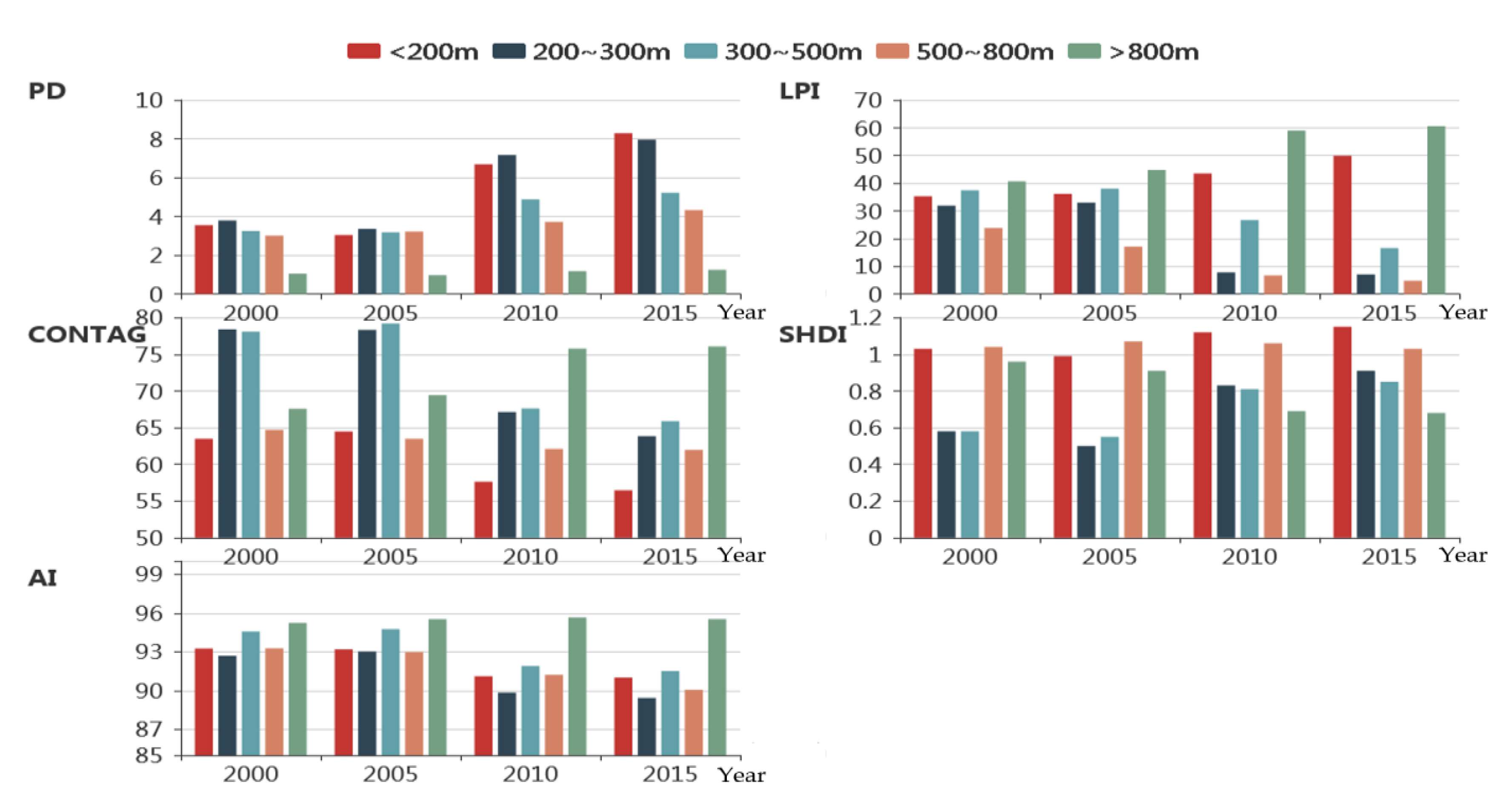
3.3. Spatial Variation in Landscape-Level Indices

3.3.1. Variation of the Landscape Index with Elevation at the Landscape Level

Except that the PD in the study area gradually decreased with increasing elevation in 2015, the elevational variation in the PD in the three other years increased first and then decreased, and the peak value was in the 200–300-m elevation range. Throughout the four periods, the LPI showed a fluctuating pattern of increase–decrease–decrease–increase with increasing elevation. The highest value was in the >800-m elevation range, and the lowest value was in the 500–800-m range. The overall CONTAG of the study area was relatively high, and it was higher in the 200–500-m elevation range than in other ranges. The SHDI of the study area had high values in two elevation ranges: <200 m and 500–800 m. The SHDI in the >800-m range was slightly lower than that in the former two ranges, and it was low and relatively stable in the range of 200–500 m. The AI of the study area was generally high, mostly above 90; elevational variation was not apparent, and the only relatively high value was in the >800-m elevation range (Figure 3).

3.3.2. Variation of the Landscape Index with Slope at the Landscape Level

In Figure 4, the PD of the study area showed a decreasing trend with increasing slope. The LPI had the highest values in the slope range of 0°–6°, and the second highest values were in the range of 6°–15° in 2000 and 2005. The LPI values were the lowest from 25°–35°. However, in 2010 and 2015, the second highest LPI values were in the >35° slope range and the lowest values were in the 15°–25° slope range. Throughout the four periods, the CONTAG and AI of the study area increased with increasing slope, while the SHDI showed the opposite variation patterns, i.e., decreased with increasing slope.

3.3.3. Variation of the Landscape Index with Aspect at the Landscape Level

In general, the aspect variation characteristics of PD were ranked as follows: gentle slope area > northeasterly aspect > southwesterly aspect > southerly aspect > northerly aspect > westerly aspect > easterly aspect > southeasterly aspect > northwesterly aspect. The PD was highest in the gentle slope area and lowest in areas with a northwesterly aspect. The LPI was the highest in the gentle slope area, followed by the southeasterly and northwesterly aspects, and lowest in areas with a northerly aspect. The CONTAG peaked in areas with a southeasterly aspect and was the lowest in the gentle slope areas and in areas with a southerly aspect. The CONTAG did not differ much among other aspects. SHDI had the highest values in the gentle slope areas and in areas with a southerly aspect, whereas the lowest values were recorded in areas with a southeasterly aspect. In 2000 and 2005, the SHDI values did not differ that much among other aspects. In 2010 and 2015, the values for the northwesterly and easterly aspects were relatively low. The AI values had low apparent values (around nine) in gentle slope areas and similar values for other aspects (65–71). The AI values were relatively high for the northwesterly and southeasterly aspects.

4. Discussion

The landscape pattern is significantly affected by natural factors, and topographic factors such as elevation, slope, and aspect directly affect the regional water and heat conditions and the intensity of human activities, and thus have a direct impact on the transformation of landscape pattern changes [2,3,31]. Elevation is one of the main factors that affect landscape changes, especially in mountainous areas [43]. As a result, cropland was mainly distributed in areas above 500 m; forestland, grassland, and unused land were highly concentrated in areas above 800 m; water bodies were mainly distributed in areas below 200 m; and about 50% of the built-up land was distributed in areas between 500 and 800 m. The areas with large composite DIs were mainly distributed in the areas above 800 m and between 500 and 800 m. The landscape indexes were also affected significantly by elevation. Elevation directly affects changes in natural conditions, such as temperature and precipitation, but also has a significant impact on human activities. The difference between natural conditions and human activities inevitably leads to the obvious vertical distribution difference of the landscape pattern with the change of altitude [44].
Slope directly affects the capacity of soil conservation and water conservation. Therefore, slope also has an important influence on landscape changes [45,46]. Change in cropland was significantly affected by slope. Forestland was mainly distributed in areas with a high slope. The change in grassland distribution along different slopes was relatively small. Water bodies and built-up land were highly concentrated in the area with low slopes. In the study area, the area with the slope range of 15°–25° is the region with frequent human activities, so it is also the region with a significant change in landscape dynamics [47]. The fragmentation of landscape pattern showed a general trend of decreasing with increasing slope, but different landscape types showed different trends. In the same slope range, the fragmentation of cropland and built-up land, which are associated with intense human activities, was higher than for other landscape types in general [48].
Aspect has an important influence on local sunshine hours and solar radiation intensity, so it also affects landscape changes [46]. In the study area, the distribution and changes of landscape differed between gentle slope areas, sunny slopes, and shady slopes. On the whole, compared with elevation and slope, the influence of slope aspect on landscape pattern differentiation was small [49].
The study of dynamic changes and spatial variation of landscape patterns is important to understand the relationship between human activities and the natural environment. The current research on landscape patterns is mostly based on landscape indices of two-dimensional information. There is still a lack of research on the spatial patterns and heterogeneity of landscape and the influence of topographic factors. Therefore, it is of great theoretical significance to carry out spatial heterogeneity studies on landscape changes in typical areas. Shizhu County is a typical mountainous area, and it is a biologically-diverse area in Chongqing. The landscape patterns of Shizhu County have undergone tremendous changes. The area’s ecological location and typical landform types add to the complexity and heterogeneity of the landscape evolution. Therefore, this paper used Shizhu County, which has typical mountainous features in the hinterland of the Three Gorges Reservoir area, as the study area, to analyze the dynamic landscape changes and spatial variation from 2000–2015 through dynamic landscape changes, landscape patterns, and geographic correlations. This will have practical value for promoting the proper use of regional land resources and sustainable development of the environment. However, as the landscape types were only classified into six categories (i.e., cropland, forestland, grassland, water bodies, built-up land, and unused land), the land-use type dynamic indices and landscape indices reflect the macrostate structural changes of the landscape with the changes of topographic factors; however, it remains difficult to reveal the microstate structural changes of the landscape [50]. Therefore, in future studies, microstate changes of the landscape in mountainous areas should be considered.

5. Conclusions

Through analysis of the dynamics and spatial heterogeneity of the landscape in Shizhu County, a typical mountainous area, we drew the following conclusions: (1) Cropland and forestland were the dominant landscape types in the study area. Cropland and grassland exhibited a significant decreasing trend, being mainly converted to forestland. An increase in forestland and built-up land was apparent. The increase in built-up land was mainly due to invasion into cropland. The increase in forestland was mainly due to conversion from cropland and grassland. Water bodies were affected by factors such as water storage in the Three Gorges Reservoir, and the area continued to increase. The change in landscape was the most drastic from 2005–2010, mainly reflected by the rapid increase in built-up land and water bodies and the rapid decrease in grassland. (2) Landscape distribution and dynamics showed apparent spatial variation. Except that water bodies were mainly distributed in the gentle slope area below 200 m elevation and 0°–6° slope, other major landscapes were concentrated at an elevation higher than 500 m, along a slope of 15°–35°, on westerly and northwesterly aspects. These areas also had the most dramatic changes in landscape. (3) The landscape indices also showed apparent spatial variation. The type-level and the landscape-level landscape indices showed more distinct variation with elevation and slope than with aspect. Different landscape types had very different variation characteristics in response to elevation, slope, and aspect.

Author Contributions

Q.C. and Y.L. designed the paper. Q.C. and C.L. collected the data and wrote the paper. Y.Y. and J.W. analyzed the data and designed the figures and tables. M.L. revised the paper. All authors have read and approved the final manuscript.

Funding

This research was funded by the National Natural Science Foundation of China (41571419).

Acknowledgments

The authors wish to thank the anonymous reviewers for their constructive comments and suggestions.

Conflicts of Interest

The authors declare no conflict of interest.

References

  1. Jia, Y.; Yan, L.; Yu, F.; Cao, L.L. Land use change and landscape pattern of typical semi-arid and arid watershed of Western China: A case study on Shiyang River Basin. Remote Sens. Inf. 2016, 31, 66–73. [Google Scholar]
  2. Zhu, D.G.; Xie, B.G.; Xiong, P. Spatial-temporal evolution of land-use pattern changes in Zhangjiajie city based on three-dimensional landscape pattern indices. Econ. Geogr. 2017, 37, 168–175. [Google Scholar]
  3. Wu, B.; Ci, L.J. Temporal and spatial patterns of landscape in the Mu Us Sandland, Northern China. Acta Ecol. Sin. 2001, 21, 191–196. [Google Scholar]
  4. Peng, B.F.; Chen, D.L.; Li, W.J.; Wang, Y.L. Stability of landscape pattern of land use: A case study of Changde. Sci. Geogr. Sin. 2013, 33, 1484–1488. [Google Scholar]
  5. Liang, X.Y.; Gu, Z.M.; Lei, M.; Wang, X. The differences between land use function and land use to reflecting the change of land use system and their impacts on landscape pattern: A case study of Lantian County in Shaanxi Province, China. J. Nat. Resour. 2014, 29, 1127–1135. [Google Scholar]
  6. He, D.; Jin, F.J.; Zhou, J. The changes of land use and landscape pattern based on Logistic-CA-Markov Model—A case study of Beijing-Tianjin-Hebei Metropolitan Region. Sci. Geogr. Sin. 2011, 31, 903–910. [Google Scholar]
  7. Lambin, E.F.; Geist, H.J. Global land-use and land-cover change: What have we learned so far? Glob. Chang. News Lett. 2001, 46, 27–30. [Google Scholar]
  8. Lambin, E.F.; Banliex, X.; Bockstael, N. Land-Use and Landcover Change (LUCC): Implementation Strategy; IGBP Report No. 48 and HDP Report No. 10; IGBP: Stochkholm, Sweden, 1999. [Google Scholar]
  9. Pijanowski, B.C.; Robinson, K.D. Rates and patterns of land use change in the Upper Great Lakes States, USA: A framework for spatial temporal analysis. Landsc. Urban Plan. 2011, 102, 102–116. [Google Scholar] [CrossRef]
  10. Bajocco, S.; De Angelis, A.; Perini, L.; Ferrara, A.; Salvati, L. The impact of land use/land cover changes on land degradation dynamics: A mediterranean case study. Environ. Manag. 2012, 49, 980–989. [Google Scholar] [CrossRef]
  11. Wang, Q.; Meng, J.J.; Mao, X.Y. Scenario simulation and landscape pattern assessment of land use change based on neighborhood analysis and auto-logistic model: A case study of Lijiang River Basin. Geogr. Res. 2014, 33, 1073–1084. [Google Scholar]
  12. Wang, L.; Li, C.C.; Ying, Q.; Cheng, X.; Wang, X.Y.; Li, X.Y.; Hu, L.Y.; Liang, L.; Yu, L.; Huang, H.B.; et al. China’s urban expansion from 1990 to 2010 determined with satellite remote. Chin. Sci. Bull. 2012, 57, 2802–2812. [Google Scholar] [CrossRef]
  13. Tong, G.C.; Lin, J.; Chen, H.; Gu, Z.Y.; Tang, P.; Zhang, J.C. Land use and landscape pattern changes and the driving force factors in Nanjing from 1986 to 2013. Res. Soil Water Conserv. 2017, 24, 240–245. [Google Scholar]
  14. Liu, M.Y.; Jiang, F.; Liu, Y. Land use pattern changes over the last two decades in Qinwangchuan area, Lanzhou, China. J. Arid Land Resour. Environ. 2016, 30, 111–116. [Google Scholar]
  15. Bonzongo, J.C.; Donkor, A.; Attibayeba, A.; Gao, J. Linking landscape development intensity within watersheds to methyl-mercury accumulation in river sediments. AMBIO 2016, 45, 196–204. [Google Scholar] [CrossRef] [PubMed]
  16. Zhang, G.K.; Deng, W.; Song, K.S.; Liu, J.P.; Zhang, L.H.; Li, F. On the land use pattern shifting in Xinkai River Basin and its ecological significance. Acta Ecol. Sin. 2006, 26, 3025–3034. [Google Scholar]
  17. Wang, L.; Wang, Y.; Cai, Y.L. An ANN-CA modeling method for land cover change in the karst area of China: A case study of Maotiao River Basin. Acta Sci. Nat. Univ. Pekin. 2012, 48, 116–122. [Google Scholar]
  18. Du, Q.; Xu, H.L.; Zhao, X.F.; Zhang, P.; Ling, H.B.; Wang, X.Y. Changing characteristics of land use/cover and landscape pattern from 1990 to 2010 in the Kaxgar River Basin, Xinjiang. J. Glaciol. Geocryol. 2014, 36, 1548–1555. [Google Scholar]
  19. Tan, J.; Zhao, S.N.; Tan, X.L.; Dong, L.; Liu, J.R.; Ji, Q.Y. Change characteristics of land use and landscape pattern in Dongting Lake during 1996–2016. Ecol. Sci. 2017, 36, 90–97. [Google Scholar]
  20. Fan, K.; Zhang, J.S.; Pei, W.J.; Yang, C.L.; Chen, Y.C.; Yu, J.X.; Zeng, W.J. Land use landscape pattern and stability analysis of three plateau major lake basins in Yunnan Province. Southwest China J. Agric. Sci. 2018, 31, 1706–1711. [Google Scholar]
  21. Liu, Y.B.; Dai, L.; Dong, Y.Y. Simulation of landscape pattern change of Poyang lake area patition. Resour. Environ. Yangtze Basin 2015, 24, 1762–1770. [Google Scholar]
  22. Jing, Y.Q.; Zhang, F.; Chen, L.H.; Zhang, Y.; Wang, X.P.; Li, Z.; Hsiang-te, K. Investigation on eco-environmental effects of land use/cover-landscape pattern and climate change in Ebinur Lake Wetland Nature Reserve. Acta Sci. Circumst. 2017, 37, 3590–3601. [Google Scholar]
  23. Liu, J.P.; Zhao, D.D.; Tian, X.Z.; Zhao, L.; Liu, J.F. Landscape pattern dynamics and driving forces analysis in the Sanjiang Plain from 1954 to 2010. Acta Ecol. Sin. 2014, 34, 3234–3244. [Google Scholar]
  24. Nian, Y.Y.; Wang, X.L.; Chen, L. Land use pattern change in Ejin Delta of Northwest China during 1930–2010. Chin. J. Appl. Ecol. 2015, 26, 777–785. [Google Scholar]
  25. Liu, Y.X.; Li, Y.B.; Yi, X.S.; Cheng, X. Spatial evolution of land use intensity and landscape pattern response of the typical basins in Guizhou Province, China. Chin. J. Appl. Ecol. 2017, 28, 3691–3702. [Google Scholar]
  26. Ren, Z.Y.; Zhang, H. Effects of land use change on landscape pattern vulnerability in Yinchuan Basin, Northwest China. Chin. J. Appl. Ecol. 2016, 27, 243–249. [Google Scholar]
  27. Peng, J.; Xu, Y.Q.; Cai, Y.L.; Xiao, H.L. The role of policies in land use/cover change since the 1970s in ecologically fragile karst areas of Southwest China: A case study on the Maotiaohe watershed. Environ. Sci. Policy 2011, 14, 408–418. [Google Scholar] [CrossRef]
  28. Huang, Q.H.; Cai, Y.L. Simulation of land use change using GIS based stochastic model: The case study of Shiqian County, Southwestern China. Stoch. Environ. Res. Risk Assess. 2007, 21, 419–426. [Google Scholar] [CrossRef]
  29. Xu, Y.Q.; Luo, D.; Peng, J. Land use change and soil erosion in the Maotiao River watershed of Guizhou Province. J. Geogr. Sci. 2011, 21, 1138–1152. [Google Scholar] [CrossRef]
  30. Li, Y.B.; Yao, Y.W.; Xie, J.; Wang, F.Y.; Bai, X.Y. Spatial-temporal evolution of land use and landscape pattern of the mountain-basin system in Guizhou Province. Acta Ecol. Sin. 2014, 32, 3257–3265. [Google Scholar]
  31. Zhang, P.; Zhou, B.T.; Yue, Q.L.; Wang, N. Analysis of small-scaled landscape patterns changes in mountain areas based on GIS—A case study of Yujin town, Qianwei County. J. Sichuan Agric. Univ. 2010, 28, 486–491. [Google Scholar]
  32. Chen, Y.R.; Xiao, W.F.; Teng, M.J.; Feng, Y. Grain size effect of landscape pattern and its response to land use change in the Three Gorges Reservoir Area. J. Nat. Resour. 2018, 33, 588–599. [Google Scholar]
  33. Jia, J.T.; Yang, H.; Zeng, X.; Zhang, Y.J. Analysis on landscape pattern of land use in a mountain city: A case study from metropolitan area in Chongqing. J. Chongqing Norm. Univ. (Nat. Sci. Ed.) 2013, 30, 35–44. [Google Scholar]
  34. Wen, Q.; Li, Q.S.; Sun, S.J. Research on the land use landscape pattern of different soil types in central-south hilly area. Res. Soil Water Conserv. 2012, 19, 90–99. [Google Scholar]
  35. Zhang, Z.M.; Luo, Q.P.; Wang, W.L.; Yin, M.; Sun, Z.H.; Ou, X.K.; Liu, X.K. A comparison of 2D and 3D landscape metrics for vegetation patterns change quantification in mountainous areas. Acta Ecol. Sin. 2010, 30, 5886–5893. [Google Scholar]
  36. Wu, Z.F.; Wei, L.Z.; Lv, Z.Q. Landscape pattern metrics: An empirical study from 2-D to 3-D. Phys. Geogr. 2012, 33, 383–402. [Google Scholar] [CrossRef]
  37. Xu, N.Y.; Guo, L.; Xue, D.Y.; Sun, S.Q. Land use structure and the dynamic evolution of ecosystem service value in Gannan region, China. Acta Ecol. Sin. 2019, 39, 1–10. [Google Scholar]
  38. Sun, W.L.; Sun, Z.G.; Tian, L.P.; Hu, X.Y. Variation and prediction of different marsh landscapes in intertidal zone of the Yellow River Delta. Acta Ecol. Sin. 2017, 37, 215–225. [Google Scholar]
  39. Angeler, D.; Viedam, O.; Sánchez-Carrillo, S.; Alvarez-Cobelas, M. Conservation issues of temporary wetland Branchiopoda (Anostraca, Notostraca: Crustacea) in a semiarid agricultural landscape: What spatial scales are relevant? Biol. Conserv. 2008, 14, 1224–1234. [Google Scholar] [CrossRef]
  40. Xu, X.R.; Xie, G.Z.; Qiu, P.H. Dynamic analysis of landscape changes in Bamen port and the surrounding lands of Hainan Province from 1964 to 2015. Acta Ecol. Sin. 2018, 38, 7458–7468. [Google Scholar]
  41. Zhang, M.; Gong, Z.N.; Zhao, W.J.; Duo, A. Landscape pattern change and the driving forces in Baiyangdian wetland from 1984 to 2014. Acta Ecol. Sin. 2016, 36, 4780–4791. [Google Scholar]
  42. Li, X.Z.; Bu, R.C.; Chang, Y.; Hu, Y.M.; Wen, Q.C.; Wang, X.G.; Xu, C.G.; Li, Y.H.; He, H.S. The response of landscape metrics against pattern scenarios. Acta Ecol. Sin. 2004, 24, 123–134. [Google Scholar]
  43. Zhao, L.H.; Wang, P.; Ouyang, X.Z.; Wu, Z.W. An analysis of the spatio-temporal variation in fractional vegetation cover and its relationship with non-climate factors in Nanchang City, China. Acta Ecol. Sin. 2016, 36, 3723–3733. [Google Scholar]
  44. Wang, L.; Mi, W.B.; Wang, X.; Chen, X.Z. Driving forces of land-use changes in exploration limited ecological zones—Xiji county, Ningxia. J. Arid Land Resour. Environ. 2019, 33, 51–57. [Google Scholar]
  45. Yang, S.H.; Hu, S.G.; Qu, S.J. Terrain gradient effect of ecosystem service value in middle reach of Yangtze River, China. Chin. J. Appl. Ecol. 2018, 29, 976–986. [Google Scholar]
  46. Wu, A.B.; Qin, Y.J.; Zhao, Y.X. Terrain composite index and its application in terrain gradient effect analysis of land use change: A case study of Taihang hilly areas. Geogr. Geo-Inf. Sci. 2018, 34, 93–99. [Google Scholar]
  47. Shao, J.M. RS-and GIS-Based Study on the Changes of Landscape Pattern in Elevation and Ecological Function Regionalization; Southwest University: Chongqing, China, 2016. [Google Scholar]
  48. Wang, F.; Shao, J.A.; Dang, Y.F. Analysis of Land use change in Shizhu County of Chongqing. Rural Econ. Sci.-Technol. 2017, 28, 4–5. [Google Scholar]
  49. Chen, Z.; Huang, Y.B.; Zhu, Z.P.; Zheng, Q.Q.; Que, C.X.; Dong, J.W. Landscape pattern evolution along terrain gradient in Fuzhou City, Fujian Province, China. Chin. J. Appl. Ecol. 2018, 29, 4135–4144. [Google Scholar]
  50. Cushman, S. Calculation of configurational entropy in complex landscapes. Entropy 2018, 20, 298. [Google Scholar] [CrossRef]
Figure 1. Map of the study area.
Sustainability 11 02131 g001
Figure 2. Map of the landscape types of Shizhu County (2000–2015).
Sustainability 11 02131 g002
Figure 3. Variation in the landscape-level landscape index with elevation in Shizhu County from 2000–2015. PD, patch density; LPI, largest patch index; CONTAG, landscape contagion; SHDI, Shannon diversity index; AI, aggregation index.
Sustainability 11 02131 g003
Figure 4. Variation in the landscape-level landscape index with slope in Shizhu County from 2000–2015.
Sustainability 11 02131 g004
Table 1. Information of Landsat images used in the paper.
Satellite/SensorPath/RowTimeBandsResolution (m)
Landsat 8 OLI_TIRS127/39Oct., 21, 20151–730
Landsat 5 TM127/39Oct., 23, 20101–5,730
Landsat 5 TM127/39Jul., 21, 20051–5,730
Landsat 5 TM127/39Aug., 09, 20061–5,730
Landsat 5 TM127/39May, 20, 20001–5,730
Table 2. Areas and ratios of different landscape types in Shizhu County from 2000–2015 (area unit: km2; ratio unit: %).
YearArea/RatioCroplandForestlandGrasslandWater BodiesBuilt-up LandUnused Land
2000area1140.871470.58387.9212.844.911.33
ratio37.848.7212.850.430.160.04
2005area1184.551530.2272.122.47.321.89
ratio39.2450.699.010.760.240.06
2010area858.522008.2683.4633.9432.741.53
ratio28.4566.532.771.121.080.05
2015area829.872034.6262.0435.2955.70.93
ratio27.4867.412.061.171.850.03
Table 3. Dynamic index of landscape changes in Shizhu County from 2000–2015 (%).
Type2000–20052005–20102010–2015
cropland 0.77−5.51−0.67
forestland0.816.250.26
grassland−5.97−13.87−5.13
water bodies14.8910.300.80
built-up land9.8269.4514.03
unused land8.42−3.81−7.84
composite DI3.8417.061.68

