Spatial Correlation and Convergence Analysis of Eco-Efficiency in China


Abstract
:1. Introduction
2. Models and Data
2.1. SBM Model
2.2. Construction and Decomposition of the Malmquist Index Model
2.3. Exploratory Spatial Data Analysis
2.4. Construction of Spatial Weighting Matrix
2.4.1. Queen Contiguity
2.4.2. Rook Contiguity
2.4.3. K-nearest Neighbors
2.4.4. Threshold Distance
2.4.5. Asymmetrical Spatial Weighting Matrix Based on the EETI-Distance Reciprocal Principle
3. Analysis of Spatial Correlation of Ecological Efficiency in Mainland China
3.1. Variables and Data Source
3.2. Comparison of Evaluation Results Based on Symmetric Spatial Weight Matrix
3.2.1. Global Spatial Autocorrelation Analysis of Eco-Efficiency in Mainland China
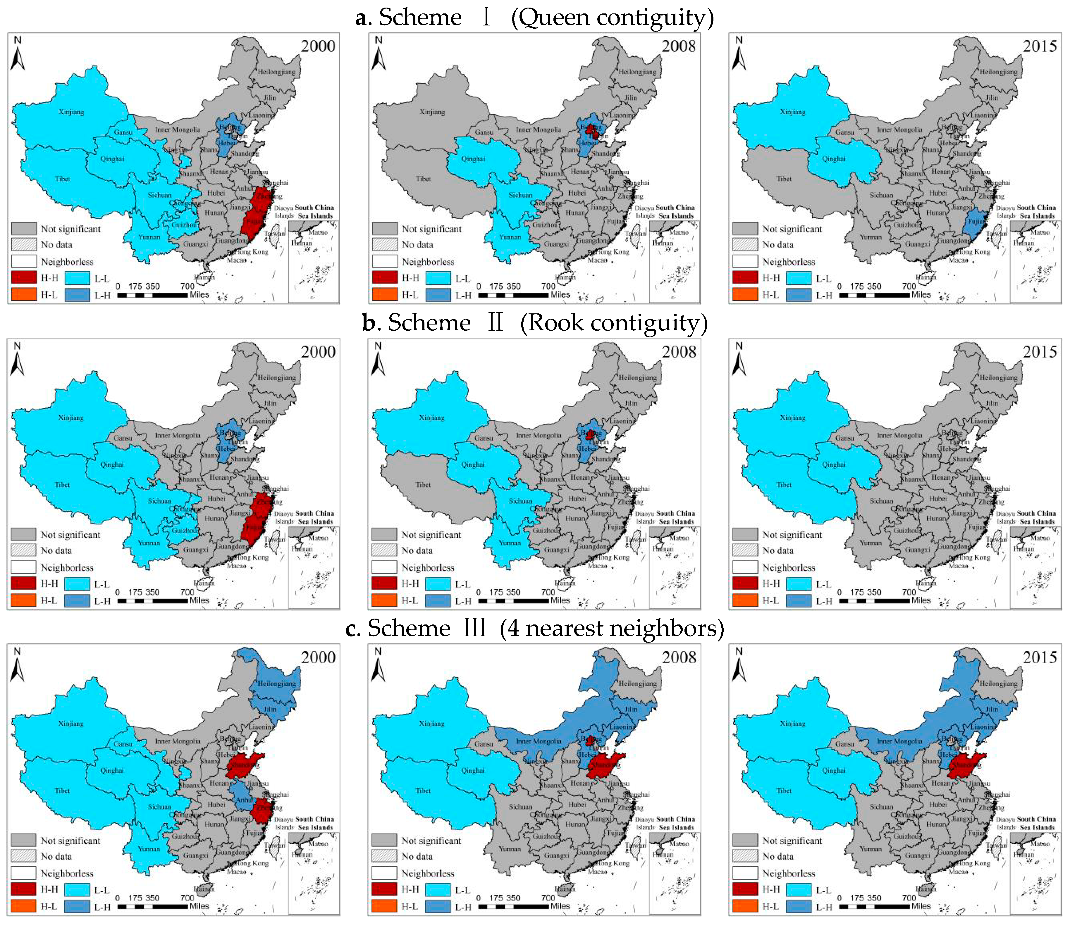
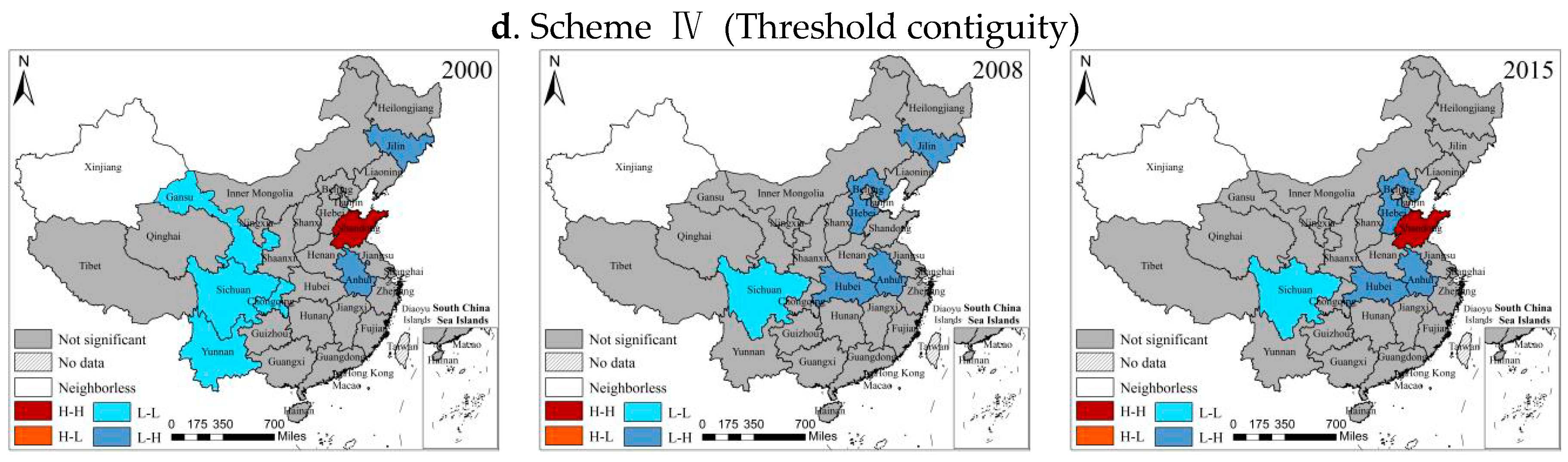
3.2.2. Local Spatial Autocorrelation Analysis of Eco-Efficiency in Mainland China
3.3. Analysis of Evaluation Results Based on Asymmetrical Spatial Weight Matrix
3.3.1. Global Spatial Autocorrelation Analysis of Eco-Efficiency in Mainland China Based on the EETI-Distance Reciprocal Principle
3.3.2. Local Spatial Autocorrelation Analysis of Eco-Efficiency in Mainland China Based on the EETI-Distance Reciprocal Principle
4. Analysis of the Convergence of Eco-Efficiency in Mainland China
4.1. Convergence Model
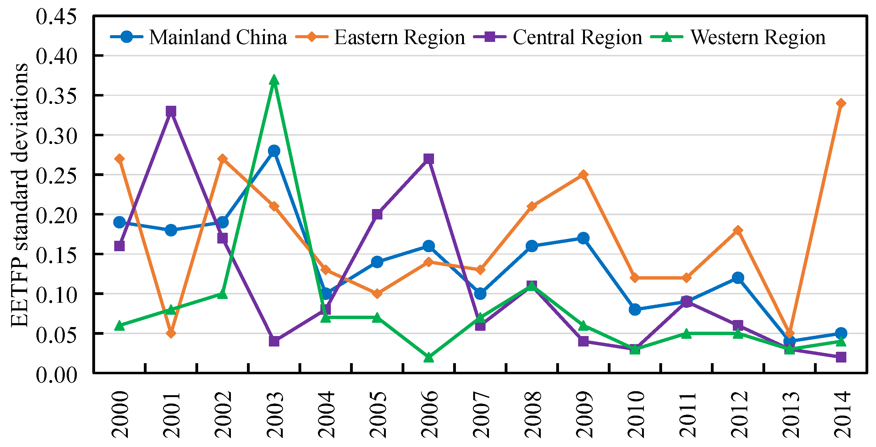
4.2. σ Convergence
4.3. Absolute β Convergence
4.4. Conditional β Convergence
5. Conclusions and Suggestions
Author Contributions
Funding
Conflicts of Interest
References
- Schaltegger, S.; Sturm, A. Ökologische Rationalität: Ansatzpunkte zur Ausgestaltung von ökologieorientierten Managementinstrumenten. Die Unternehmung 1990, 44, 273–290. [Google Scholar]
- World Business Council for Sustainable Development (WBCSD). Eco-Efficient Leadership for Improved Economic and Environmental Performance; WBCSD: Conches-Geneva, Switzerland, 1996. [Google Scholar]
- Organisation for Economic Co-operation and Development. Eco-Efficiency; OECD: Geneva, Switzerland, 1998; pp. 7–11. [Google Scholar]
- Saling, P.; Kicherer, A.; Dittrich-Krämer, B.; Wittlinger, R.; Zombik, W.; Schmidt, I.; Schrott, W.; Schmidt, S. Eco-efficiency Analysis by BASF: The Method. Int. J. Life Cycle Assess. 2002, 7, 203–218. [Google Scholar] [CrossRef]
- United Nations Conference on Trade and Development (UNCTD). Integrating Environmental and Financial Performance at the Enterprise Level: A Methodology for Standardizing Eco-Efficiency Indicators; United Nations Publication: New York, NY, USA, 2003; pp. 29–30. [Google Scholar]
- An, V.; Spirinckx, C.; Geerken, T. Life cycle assessment and eco-efficiency analysis of drinking cups used at public events. Int. J. Life Cycle Assess. 2010, 15, 221–230. [Google Scholar]
- Van Caneghem, J.; Block, C.; Cramm, P.; Mortier, R.; Vandecasteele, C. Improving eco-efficiency in the steel industry: The ArcelorMittal Gent case. J. Clean. Prod. 2010, 18, 807–814. [Google Scholar] [CrossRef]
- Michelsen, O.; Fet, A.M.; Dahlsrud, A. Eco-efficiency in extended supply chains: A case study of furniture production. J. Environ. Manag. 2006, 79, 290–297. [Google Scholar] [CrossRef]
- Neto, J.Q.F.; Walther, G.; Bloemhof, J.; van Nunen, J.A.E.E.; Spengler, T. A Methodology for Assessing Eco-Efficiency in Logistics Networks. Eur. J. Oper. Res. 2009, 193, 670–682. [Google Scholar] [CrossRef]
- Egilmez, G.; Gumus, S.; Kucukvar, M.; Tatari, O. A Fuzzy Data Envelopment Analysis Framework for Dealing with Uncertainty Impacts of Input-Output Life Cycle Assessment Models on Eco-efficiency Assessment. J. Clean. Prod. 2016, 129, 622–636. [Google Scholar] [CrossRef]
- Martín-Gamboa, M.; Iribarren, D.; Dufour, J. Environmental impact efficiency of natural gas combined cycle power plants: A combined life cycle assessment and dynamic data envelopment analysis approach. Sci. Total Environ. 2018, 615, 29–37. [Google Scholar] [CrossRef] [PubMed]
- Lahouel, B.B. Eco-efficiency analysis of French firms: A data envelopment analysis approach. Environ. Econ. Policy Stud. 2016, 18, 395–416. [Google Scholar] [CrossRef]
- Wursthorn, S.; Poganietz, W.R.; Schebek, L. Economic–environmental monitoring indicators for European countries: A disaggregated sector-based approach for monitoring eco-efficiency. Ecol. Econ. 2011, 70, 487–496. [Google Scholar] [CrossRef]
- Van Middelaar, C.E.; Berentsen, P.B.M.; Dolman, M.A.; de Boer, I.J.M. Eco-efficiency in the production chain of Dutch semi-hard cheese. Livest. Sci. 2011, 139, 91–99. [Google Scholar] [CrossRef]
- Maia, R.; Silva, C.; Costa, E. Eco-efficiency assessment in the agricultural sector: The Monte Novo irrigation perimeter, Portugal. J. Clean. Prod. 2016, 138, 217–228. [Google Scholar] [CrossRef]
- Ullah, A.; Perret, S.R.; Gheewala, S.H.; Soni, P. Eco-efficiency of cotton-cropping systems in Pakistan: An integrated approach of life cycle assessment and data envelopment analysis. J. Clean. Prod. 2016, 134, 623–632. [Google Scholar] [CrossRef]
- Chen, L.M.; Wang, W.P.; Wang, B. Economic Efficiency, Environmental Efficiency and Eco-efficiency of the So-called Two Vertical and Three Horizontal Urbanization Areas: Empirical Analysis Based on HDDF and Co-Plot Method. China Soft Sci. 2015, 2, 96–109. [Google Scholar]
- Peng, H.; Zhang, J.H.; Lu, L.; Yan, B.J.; Xiao, X.; Han, Y. Eco-efficiency and its determinants at a tourism destination: A case study of Huangshan National Park, China. Tour. Manag. 2017, 60, 201–211. [Google Scholar] [CrossRef]
- Li, Z.; Ouyang, X.L.; Du, K.R.; Zhao, Y. Does government transparency contribute to improved eco-efficiency performance? An empirical study of 262 cities in China. Energy Policy 2017, 110, 79–89. [Google Scholar] [CrossRef]
- Wang, S.J.; Ma, Y.Y. Influencing factors and regional discrepancies of the efficiency of carbon dioxide emissions in Jiangsu, China. Ecol. Indic. 2018, 90, 460–468. [Google Scholar] [CrossRef]
- Ren, S.G.; Li, X.L.; Yuan, B.L.; Li, D.Y.; Chen, X.H. The effects of three types of environmental regulation on eco-efficiency: A cross-region analysis in China. J. Clean. Prod. 2018, 173, 245–255. [Google Scholar] [CrossRef]
- Zhang, J.X.; Liu, Y.M.; Chang, Y.; Zhang, L.X. Industrial eco-efficiency in China: A provincial quantification using three-stage data envelopment analysis. J. Clean. Prod. 2017, 143, 238–249. [Google Scholar] [CrossRef]
- Huang, J.H.; Xia, J.J.; Yu, Y.T.; Zhang, N. Composite eco-efficiency indicators for China based on data envelopment analysis. Ecol. Indic. 2018, 85, 674–697. [Google Scholar] [CrossRef]
- Li, J.; Deng, C.X.; Zhang, S.T. The evaluation and dynamic analysis on regional eco-efficiency based on Non-parametric Distance Function. J. Arid Land Resour. Environ. 2015, 29, 19–23. [Google Scholar]
- Cheng, J.H.; Sun, Q.; Guo, M.J.; Xu, W.Y. Research on Regional Disparity and Dynamic Evolution of Eco-efficiency in China. China Popul. Resour. Environ. 2012, 24, 47–57. [Google Scholar]
- Bai, Y.P.; Deng, X.Z.; Jiang, S.J.; Zhang, Q.; Wang, Z. Exploring the relationship between urbanization and urban eco-efficiency: Evidence from prefecture-level cities in China. J. Clean. Prod. 2018, 195, 1487–1496. [Google Scholar] [CrossRef]
- Charnes, A.; Cooper, W.W.; Rhodes, E. Measuring the efficiency of decision making units. Eur. J. Oper. Res. 1978, 2, 429–444. [Google Scholar] [CrossRef]
- Tone, K. A slacks-based measure of super-efficiency in data envelopment analysis. Eur. J. Oper. Res. 2002, 143, 32–41. [Google Scholar] [CrossRef] [Green Version]
- Tone, K. A slacks-based measure of efficiency in data envelopment analysis. Eur. J. Oper. Res. 2001, 130, 498–509. [Google Scholar] [CrossRef] [Green Version]
- Färe, R.; Grosskopf, S.; Noh, D.W.; Weber, W. Characteristics of a polluting technology: Theory and practice. J. Econom. 2005, 126, 469–492. [Google Scholar] [CrossRef]
- Wang, H.F.; Shi, Y.S.; Ying, C.Y. Land use efficiencies and their changes of Shanghai’s development zones employing DEA model and Malmquist productivity index. Geogr. Res. 2014, 33, 1636–1646. [Google Scholar]
- Sawada, M. Global Spatial Autocorrelation Indices-Moran’s I, Geary’s C and the General Cross-Product Statistic; Laboratory for Paleoclimatology and Climatology at the University of Ottawa: Ottawa, ON, Canada, 2004. [Google Scholar]
- Moran, P.A.P. The statistical analysis of the Canadian Lynx cycle. Aust. J. Zool. 1953, 1, 291–298. [Google Scholar] [CrossRef]
- Parent, O.; Lesage, J.P. Using the variance structure of the conditional autoregressive spatial specification to model knowledge spillovers. J. Appl. Econom. 2008, 23, 235–256. [Google Scholar] [CrossRef]
- Dey-Chowdhury, S. Methods explained: Perpetual Inventory Method (PIM). Econ. Labour Mark. Rev. 2008, 2, 48–52. [Google Scholar] [CrossRef] [Green Version]
- Shan, H.J. Re-estimating the capital stock of China: 1952–2006. J. Quant. Tech. Econ. 2008, 25, 17–31. [Google Scholar]
- Wu, J.D.; Li, N.; Shi, P. Benchmark wealth capital stock estimations across China’s 344 prefectures: 1978 to 2012. China Econ. Rev. 2014, 31, 288–302. [Google Scholar] [CrossRef]
- Berlemann, M.; Wesselhöft, J.E. Estimating Aggregate Capital Stocks Using the Perpetual Inventory Method. Rev. Econ. 2014, 65, 1–34. [Google Scholar] [CrossRef]
- Quah, D. Galton’s Fallacy and Tests of the Convergence Hypothesis. Scand. J. Econ. 1993, 95, 427–443. [Google Scholar] [CrossRef]
- Sala-I-Martin, X.X. Regional cohesion: Evidence and theories of regional growth and convergence. Eur. Econ. Rev. 1994, 40, 1325–1352. [Google Scholar] [CrossRef]


| Year | 2000 | 2002 | 2004 | 2006 | 2008 | 2010 | 2012 | 2014 | 2015 |
|---|---|---|---|---|---|---|---|---|---|
| Obs. | 31 | 31 | 31 | 31 | 31 | 31 | 31 | 31 | 31 |
| Water footprint (in 100 million m3) | |||||||||
| mean | 337.60 | 339.54 | 336.21 | 351.85 | 352.47 | 368.69 | 359.20 | 398.95 | 398.85 |
| std. | 221.62 | 222.65 | 222.84 | 231.89 | 230.40 | 244.69 | 237.54 | 265.45 | 265.75 |
| min | 13.92 | 14.66 | 12.90 | 16.98 | 17.82 | 18.84 | 17.57 | 24.60 | 25.17 |
| max | 851.28 | 817.14 | 863.06 | 965.79 | 962.59 | 1081.67 | 1083.41 | 1182.21 | 116.28 |
| Labor force (in 10 thousand persons) | |||||||||
| mean | 2032.37 | 2054.55 | 2131.96 | 2290.42 | 2338.94 | 2466.54 | 2504.70 | 2658.39 | 2671.13 |
| std. | 1419.37 | 1413.41 | 1460.19 | 1618.90 | 1619.29 | 1703.29 | 1778.02 | 1787.39 | 1794.14 |
| min | 123.40 | 128.80 | 134.80 | 148.20 | 160.40 | 175.00 | 202.10 | 214.00 | 235.00 |
| max | 5571.70 | 5522.00 | 5587.40 | 5960.00 | 5835.50 | 6041.60 | 6554.30 | 6607.00 | 6636.00 |
| Fixed-asset investment (in 100 million RMB) a | |||||||||
| mean | 4256.35 | 5958.27 | 8880.29 | 14,209.95 | 21,738.55 | 32,829.04 | 46,654.70 | 61,328.10 | 67,968.82 |
| std. | 3199.16 | 4445.54 | 6781.26 | 10,657.41 | 15,518.34 | 22,747.40 | 31,142.32 | 39,595.44 | 435,533.41 |
| min | 78.70 | 213.48 | 569.15 | 918.82 | 1324.68 | 2251.98 | 3136.48 | 4711.90 | 5217.04 |
| max | 12,267.43 | 16,548.13 | 25,472.23 | 41,820.05 | 60,337.81 | 91,441.69 | 125,471.11 | 161,918.16 | 179,884.17 |
| Cost of resource and environment (in 100 million RMB) | |||||||||
| mean | 2290.03 | 2414.45 | 2537.97 | 2742.56 | 3015.37 | 3401.47 | 3903.69 | 4494.86 | 4521.03 |
| std. | 2887.47 | 3064.18 | 3264.74 | 3507.48 | 3840.88 | 4315.43 | 4948.16 | 5797.25 | 5849.13 |
| min | 67.32 | 81.76 | 78.97 | 82.97 | 91.40 | 95.15 | 108.80 | 233.98 | 134.32 |
| max | 12,473.96 | 13,176.42 | 13,918.91 | 14,992.44 | 16,225.47 | 17,916.77 | 20,918.61 | 23,619.78 | 23,948.83 |
| Construction land area (in km2) | |||||||||
| mean | 116.80 | 99.11 | 101.78 | 104.41 | 106.54 | 112.26 | 117.98 | 122.67 | 124.49 |
| std. | 74.67 | 58.32 | 59.64 | 61.13 | 61.88 | 64.90 | 68.06 | 70.50 | 71.33 |
| min | 8.64 | 5.49 | 6.13 | 6.50 | 6.70 | 9.54 | 12.38 | 14.15 | 14.50 |
| max | 292.59 | 230.25 | 238.36 | 246.30 | 251.10 | 261.22 | 271.34 | 279.21 | 282.01 |
| GDP (in 100 million RMB) a | |||||||||
| mean | 3135.78 | 3923.95 | 5591.79 | 7627.81 | 10,776.89 | 14,545.55 | 18,719.43 | 21,808.46 | 22,935.83 |
| std. | 2462.39 | 3159.95 | 4604.09 | 6561.43 | 8736.92 | 11,358.44 | 13,846.73 | 16,320.80 | 17,481.28 |
| min | 117.46 | 171.89 | 225.98 | 301.38 | 398.44 | 520.91 | 716.41 | 932.61 | 1041.40 |
| max | 9662.23 | 13,612.10 | 19,443.50 | 27,103.18 | 35,567.59 | 46,677.51 | 55,728.78 | 65,973.84 | 70,972.52 |
| Gray water footprint (in 100 million m3) | |||||||||
| mean | 159.57 | 155.79 | 161.73 | 168.08 | 147.29 | 144.15 | 143.75 | 140.29 | 137.93 |
| std. | 102.68 | 102.33 | 103.01 | 105.28 | 88.20 | 86.71 | 83.16 | 81.57 | 79.69 |
| min | 31.16 | 24.99 | 25.12 | 19.29 | 15.54 | 11.48 | 12.37 | 8.02 | 4.98 |
| max | 421.79 | 400.56 | 410.41 | 434.14 | 358.95 | 351.83 | 334.35 | 329.84 | 322.41 |
| Environmental pollutants (kilo tons) | |||||||||
| mean | 2159.50 | 1868.98 | 1941.12 | 1866.38 | 1479.47 | 1277.81 | 1123.54 | 1217.60 | 1113.84 |
| std. | 1981.97 | 1754.05 | 1757.67 | 1429.80 | 1011.91 | 760.15 | 703.64 | 783.78 | 717.16 |
| min | 51.73 | 40.00 | 45.18 | 45.20 | 40.06 | 45.01 | 10.80 | 18.14 | 22.50 |
| max | 8658.11 | 8955.30 | 9373.22 | 7539.02 | 4834.86 | 3188.82 | 2,577,100.00 | 2987.59 | 2683.80 |
| Weight Schemes | Statistics | 2000 | 2002 | 2004 | 2006 | 2008 | 2010 | 2012 | 2014 | 2015 |
|---|---|---|---|---|---|---|---|---|---|---|
| Scheme I Queen contiguity | GMI | 0.460 *** | 0.339 *** | 0.299 *** | 0.294 *** | 0.308 *** | 0.294 *** | 0.262 *** | 0.276 ** | 0.277 ** |
| p-value | 0.001 | 0.004 | 0.005 | 0.008 | 0.009 | 0.010 | 0.010 | 0.014 | 0.011 | |
| Scheme II Rook contiguity | GMI | 0.460 *** | 0.339 *** | 0.299 *** | 0.294 ** | 0.308 *** | 0.294 *** | 0.262 ** | 0.276 *** | 0.277 *** |
| p-value | 0.001 | 0.005 | 0.005 | 0.011 | 0.006 | 0.008 | 0.012 | 0.009 | 0.010 | |
| Scheme III 4-nearest neighbors | GMI | 0.313 *** | 0.226 ** | 0.134 * | 0.146 ** | 0.116 * | 0.083 | 0.041 | 0.043 | 0.039 |
| p-value | 0.007 | 0.015 | 0.077 | 0.044 | 0.084 | 0.133 | 0.215 | 0.197 | 0.206 | |
| Scheme IV Threshold contiguity | GMI | 0.114 ** | 0.092 ** | 0.055 | 0.022 | 0.012 | 0.012 | −0.001 | -0.006 | −0.008 |
| p-value | 0.034 | 0.043 | 0.109 | 0.182 | 0.211 | 0.249 | 0.753 | 0.688 | 0.720 |
| Weight Scheme | Statistics | 2000 | 2001 | 2002 | 2003 | 2004 | 2005 | 2006 | 2007 |
| Scheme V (EETI-distance reciprocal) | GMI | 0.108 *** | 0.096 *** | 0.091 *** | 0.089 *** | 0.044 ** | 0.083 *** | 0.052 ** | 0.090 *** |
| Z-value | 3.639 | 3.340 | 3.198 | 3.162 | 1.989 | 2.998 | 2.205 | 3.185 | |
| p-value | 0.000 | 0.000 | 0.001 | 0.001 | 0.023 | 0.001 | 0.014 | 0.001 | |
| Statistic | 2008 | 2009 | 2010 | 2011 | 2012 | 2013 | 2014 | 2015 | |
| GMI | 0.085 *** | 0.071 *** | 0.074 *** | 0.065 *** | 0.061 *** | 0.064 *** | 0.060 *** | 0.059 *** | |
| Z-value | 3.045 | 2.678 | 2.778 | 2.543 | 2.439 | 2.504 | 2.418 | 2.381 | |
| p-value | 0.001 | 0.004 | 0.003 | 0.006 | 0.007 | 0.006 | 0.008 | 0.009 |
| Statistics | Regions | |||
|---|---|---|---|---|
| Mainland China | Eastern Region | Central Region | Western Region | |
| Constant | 0.028 | 0.012 | 0.087 | 0.005 |
| (0.810) | (0.714) | (1.201) | 0.223 | |
| β | −0.150 *** | −0.219 ** | −0.102 | −0.026 |
| (−3.017) | (−2.562) | (−1.093) | (−0.322) | |
| R2 | 0.098 | 0.360 | 0.0700 | 0.098 |
| Statistics | Regions | |||
|---|---|---|---|---|
| Mainland China | Eastern Region | Central Region | Western Region | |
| Constant | 0.068 | 0.025 | 0.265 *** | −0.127 |
| (0.643) | (0.071) | (2.943) | (−1.242) | |
| β | −0.182 *** | −0.269 *** | −0.314 *** | −0.067 |
| (−3.692) | (−3.272) | (−3.101) | (−0.824) | |
| PESV | 1.04 × 10⁻⁷ | −4.77 × 10⁻⁵ | −0.624 *** | 3.60 × 10⁻⁷ |
| (0.221) | (−0.734) | (−3.322) | (1.357) | |
| PGDP | 3.64 × 10⁻⁶ *** | 1.25 × 10⁻⁵ *** | 0.076 | 1.14 × 10⁻⁶ |
| (3.29) | (3.195) | (0.367) | (0.892) | |
| FDI | 6.25 × 10⁻⁵ | 2.72 × 10⁻⁵ | 0.064 | 2.19 × 10⁻⁴ |
| (1.613) | (0.483) | (1.638) | (1.156) | |
| R&D | −2.86 × 10⁻⁴ *** | −4.59 × 10⁻⁴ *** | 0.443 *** | −4.18 × 10⁻⁴ |
| (−2.872) | (−2.823) | (7.052) | (−1.116) | |
| PTI | −0.202 | −0.287 | −0.811 | 0.225 |
| (−0.796) | (−0.425) | (−1.416) | (0.876) | |
| EETI | 0.002 | 0.006 *** | 0.080 *** | 0.005 |
| (1.923) | (2.654) | (3.854) | (0.512) | |
| RECGp | −0.001 | 0.820 | −1.218 *** | −0.001 |
| (0.647) | (1.623) | (−3.547) | (−0.663) | |
| R2 | 0.735 | 0.716 | 0.927 | 0.348 |
© 2019 by the authors. Licensee MDPI, Basel, Switzerland. This article is an open access article distributed under the terms and conditions of the Creative Commons Attribution (CC BY) license (http://creativecommons.org/licenses/by/4.0/).
Share and Cite
Zheng, D.; Hao, S.; Sun, C.; Lyu, L. Spatial Correlation and Convergence Analysis of Eco-Efficiency in China. Sustainability 2019, 11, 2490. https://doi.org/10.3390/su11092490
Zheng D, Hao S, Sun C, Lyu L. Spatial Correlation and Convergence Analysis of Eco-Efficiency in China. Sustainability. 2019; 11(9):2490. https://doi.org/10.3390/su11092490
Chicago/Turabian StyleZheng, Defeng, Shuai Hao, Caizhi Sun, and Leting Lyu. 2019. "Spatial Correlation and Convergence Analysis of Eco-Efficiency in China" Sustainability 11, no. 9: 2490. https://doi.org/10.3390/su11092490