Photogrammetry for Concentrating Solar Collector Form Measurement, Validated Using a Coordinate Measuring Machine

Abstract

Concentrating solar power systems currently have a high capital cost when compared with other energy generating systems. The solar energy is captured in the form of thermal energy rather than direct electrical, which is attractive as thermal energy is more straightforward and currently more cost-effective to store in the amounts required for extended plant operation. It is also used directly as industrial process heat, including desalination and water purification. For the technology to compete against other generating systems, it is crucial to reduce the electrical energy cost to less than $0.10 per kilowatt-hour. One of the significant capital costs is the solar field, which contains the concentrators. Novel constructions and improvements to the durability and lifetime of the concentrators are required to reduce the cost of this field. This paper describes the development and validation of an inexpensive, highly portable photogrammetry technique, which has been used to measure the shape of large mirror facets for solar collectors. The accuracy of the technique has been validated to show a whole surface measurement capability of better than 100 μm using a large coordinate measuring machine. Qualification of facets of the MATS plant was performed during its installation phase, giving results of the shape, slope and intercept errors over each facet.

1. Introduction

For CSP to compete with other energy sources, it is important to reduce the cost as much as possible. A significant proportion of the cost of a plant is the solar collector field, which is made up of large areas of mirrors. The focussing shape of these mirrors must be precisely manufactured and maintained during the life of the plant to extract the maximum energy. The shape for parabolic trough collectors, which focus at a linear receiver, is affected by external forces such as wind, thermal expansion, and gravity. Understanding and predicting how the shape will change over time is key in determining the efficiency over the lifetime of the plant. Identifying and mitigating such factors during manufacture, by modifying the supporting structure design, and during maintenance, by continuing to adjust the mirrors over their life, will lead to a more efficient and more cost-effective plant.

Variations in the shape of the mirrors cause local slope errors. The sun itself has an angular size of approximately 3 mrad and combining this dispersion with the slope errors will cause the light to be reflected along a different path and potentially miss the absorber tube [1]. The shape and any errors present are principally determined by the support structure holding the mirror facets. Each mirror facet is supported independently of the adjacent facets, typically by four to six support points. If this structure is inaccurately made or misaligned, then this will place stress onto the mirror facets, bending and distorting their shape [2].

Errors in the form of the mirror may be reduced by making design changes to the collector itself or the supporting structure. Different reflective materials and constructions may be used, for example, thin films on metal sheeting [3] or different thicknesses of glass with various backing structures, such as full panel moulds [4]. The number of connection points between mirror and steel structure may be changed, or alternatives to steel may be found to provide a more stable structure for the mirrors. However, any method used needs to be subjected to analysis to investigate the potential gain versus cost, added maintenance or environmental impact from using specialized materials. The specific mirror facets described here are novel in that they are constructed from a 1 mm thick back-silvered glass, mounted onto a 3 mm pre-formed backing. Mirror facets typically in operation are 4 mm thick back-silvered glass with protective paint layers.

Shape Measurement Methods

In order to determine the amount of light that reaches the absorber tube, it is necessary to know the slope at each point on the mirror [5]. This local slope may be directly measured at many points on the mirror surface, or it may be calculated from knowing the spatial position of points on the mirror surface and interpolating between these points. The slope may typically have an error of 1 to 5 mrad [6] and the spatial position an error of up to 5 mm. To calculate slope errors to the required level, it is necessary to measure the spatial position to an accuracy of better than 100 μm. There are many methods available to evaluate the surface of the mirrors [7]. Slope measurement methods currently implemented include pattern reflection techniques, such as deflectometry and laser reflection techniques, such as VSHOT. One method of deflectometry is to use a known pattern, such as linear stripes, and to view this pattern by reflection in the mirror [8,9,10]. The pattern will be distorted by the shape of the mirror, and so by calculating the difference between known and reflected patterns, the shape of the mirror is determined. A second deflectometry method uses the reflection of the absorber tube in the mirror to determine the slope errors [11]. This has the advantage of not requiring specific patterns and projectors and also calculates the slope error based on the intended path of the sunlight. The VSHOT technique utilizes the reflection of a laser beam from a known location to a screen [12]. The position of the laser spot on the screen, combined with a precise geometry of the system allows the slope to be calculated at the reflection position on the mirror. This method has high accuracy, but is limited by the time required for multiple laser scans.

Photogrammetry may be used for measuring the spatial coordinates of a number of points on the mirror surface, and has previously been shown to be suitable for use with large parabolic trough collectors and has been used for other large surfaces as well, such as gossamer spacecraft [13,14]. It is a highly scalable technique, from fine detail over a small surface area of interest, up to whole mirror troughs and support joints. Photogrammetry is highly portable; targets are attached to the mirrors and photographs are taken with a conventional camera from many angles. These photographs are then fed into a computer and software is used to analyze the different perspectives in the images and to determine the relative positions of the target points.

Thus far, photogrammetry for CSP has used scale bars to set the scale of the generated point cloud and also as an accuracy check, where measurements of known bars are compared against their true values [2,13,15]. Or alternatively using internal error estimations generated by the photogrammetry software [16]. The method presented in this paper uses a whole surface comparison method for the validation of the developed photogrammetry technique. Here, a point cloud over the whole surface of a parabolic trough facet is measured with a coordinate measuring machine, which has a high traceable accuracy. This whole surface point cloud is then compared against the point cloud measured through photogrammetry. Thus the accuracy of photogrammetry can be determined taking into account the whole surface, not only a few discrete points.

2. Methodology

Photogrammetry must be validated to an accuracy of better than 100 μm to achieve the capability of measuring the millimetre scale distortions present in the mirrors. This validation was done by comparing the results of measurements done on a mirror surface using both the coordinate measuring machine (CMM) and photogrammetry. This surface was undisturbed between the two sets of measurements, therefore the much higher accuracy CMM can be said to produce the ‘true’ surface. Thus, the departures from this ‘true’ surface, which are measured by photogrammetry, give the accuracy of photogrammetry with respect to the CMM. The accuracy of photogrammetry is dependent on the camera settings and procedures used during measurement. These factors were optimized prior to the validation against the CMM.

2.1. Equipment

There are three main pieces of equipment needed for photogrammetry measurements: the camera, the software and the targets. The camera used was an 18MPixel Canon EOS 600D DSLR, which has a stable optical configuration and all its settings are manually controlled. High-resolution images are used so that the targets are clearly distinguished, and the central point of the target is accurately found by the centering algorithm within the software. The angles from the surface being photographed should be sufficient to allow triangulation, but not too high as to produce highly elliptical target images as this will reduce their effective size and may not be identified correctly. The photogrammetry software chosen was PhotoModeler from EOS Systems Inc. This software allows an automatic project to be set up where the photographs are loaded, and the points are automatically marked, referenced, and the solution found with minimal user input.

Coded targets are included in this automatic process, as they may be uniquely identified by rings surrounding the central point. The targets are black and white coded rings printed onto static cling vinyl sheets. These have high contrast against their background to enable the centering algorithm to be accurate to the sub-pixel level [17,18]. An alternative to the printed targets would be retroreflecitve targets [19,20,21]. Printed targets have the advantage of the flexibility of varying sizes, patterns, and point density as well as being disposable and cheap. Customization of the size, spacing, and arrangement of the targets is used to optimize the accuracy of photogrammetry depending on the object measured. The use of static cling vinyl sheets removes the requirement to clean any adhesive residue from the mirror surface following the removal of the targets.

The CMM is a Leitz PMM-F moving bridge configuration designed with a minimized moving mass comprising the Z-ram and upper bridge section. The main body of the CMM is constructed from granite, which has high stiffness, high thermal mass, and low thermal expansion. The moving bridge x-axis is controlled by dual ball spindle drives with two measurement scales to increase the precision of the system. The Z-ram itself is ceramic with a Leitz LSP-S2 probe system which may accommodate stylus extensions up to 800 mm in length. It has a measurement volume of 3 m × 2 m × 1 m and is located in a temperature and humidity controlled laboratory in the Cranfield University Precision Engineering Institute where it is primarily used for measurements of large optical components. The CMM has a traceable maximum permissible error defined as $\pm 1.9 \mathsf{\mu }\mathrm{m}+L/400$, where L, the longest length measured, is in millimeters. Over the mirror panel’s diagonal of $L=2\mathrm{m}$ this equals $\pm 6.9 \mathsf{\mu }\mathrm{m}$ calibrated accuracy error. The large measurement volume capability makes it ideal for measuring the 1.6 m × 1.2 m × 0.3 m mirror facets. It is fully programmable and can measure points automatically enabling high numbers and densities of points on complex free form surfaces while maintaining speed and accuracy.

2.2. Camera Settings Optimisation

The camera settings that were optimized for increased accuracy of photogrammetry were principally the aperture size and the shutter speed.

The aperture size controls the depth of focus of the image, which is a measure of the closest and furthest distances between which the image will have an acceptable level of focus. This is important as all targets on the mirror facet, which is 2 m along its diagonal, should be within this depth of focus to have their maximum sharpness and so their optimal identification and centering. If the depth of focus is too small, then the furthest and nearest points will be out of focus. However, if the depth of focus is too large all the points as a whole will gain an amount of blur affecting the accuracy.

The shutter speed affects the amount of light that the camera sensor receives from the object, and also affects the amount of motion blur, which may result from the camera being hand-held. The use of a tripod or fixed camera system is avoided in this technique to maximize its flexibility and portability. A faster shutter, with less time open, will result in less light striking the sensor and also a reduction in the movement that occurs while the shutter is open. This acts to increase the contrast of the targets and also reduce the blurring due to motion. However, if the shutter is too fast, the white parts of the targets will also start to reduce, diminishing the contrast again. A flash may also be necessary; depending on the lighting conditions, to increase the amount of light received from the target and so the contrast of the target.

In calculating the positions of the target points, the software must determine the precise location of the camera for each photograph based on the variations between each image. It is, therefore, necessary for the software to be calibrated for the inner optics of the camera and any lens distortions that may be present. This means that the camera must have a fixed zoom level and focus for each image and the camera should be of good quality with stable and configurable optics and not to rely on autofocus features. The software can adjust the lens distortion parameters to improve the point positions and reduce the error between photographs. This has the advantage over other calibration techniques of utilizing the same conditions under which the measurement photographs are taken.

The parameters calculated during the camera calibration are the exact focal length f, the radial distortion, and the decentering distortion. The radial distortion is radially symmetric around the principal point, which describes the center of the lens. A point that is found to be a radial distance r from the principal point must be corrected by an amount $dr$ such that the corrected X and Y components are given by $X_c=X(1+dr)$ and $Y_c=Y(1+dr)$ where $dr=K_1{r}^2+K_2{r}^4+K_3{r}^6$. $K_1$, $K_2$ and $K_3$ are the radial distortion parameters calculated by the software. The decentring distortion is much smaller than the radial lens distortion but is necessary for the highest accuracy. This describes the offset of the principal point from its ideal position, such that the corrections applied in X and Y are given by $d{p}_X=P_1(r^2+2X^2)+2P_{2}XY$ and $d{p}_Y=P_2(r^2+2Y^2)+2P_{1}XY$ respectively, where $P_1$ and $P_2$ are the decentring correction parameters also calculated within the software. The accuracy of photogrammetry may be validated using a CMM as shown in Figure 1, which is capable of measurements to much higher accuracy than photogrammetry and is traceable to international standards. There are a wide variety of sizes and configurations of CMMs, of which the bridge configuration CMM used for this paper offers higher levels of precision. A machine-driven probe is touched onto the surface, and its location is recorded by measurement transducers along three orthogonal axes. A point map of surface locations is then built from these measurements. This method is very well suited to measuring large reflective parabolic trough facets due to the large measurement volume and contact probing. Though such machines are not portable, due to their large size and the requirement for stable environments, they can be used for laboratory-based validation of other less accurate but more portable techniques, including photogrammetry.

The method of photogrammetry measurements is not standardized and depends upon the particular object and environment under test. Key elements of the method are the number of photographs, the number, and size of targets, the distance to the targets and positions that the photographs are taken from. These elements should all be tested to optimize the photogrammetry procedure; however, some can be approximately calculated prior to testing.

Measurements were performed using points that were measurable with both photogrammetry and the CMM to establish the accuracy of photogrammetry and the effect of changing the camera settings. These points were created using twenty-five 10 mm white ceramic spheres arranged in a fixed grid on the CMM table. These spheres are reflective and have high contrast against the background, which was blackened. Photogrammetry identifies the spheres as circular targets, and so the center of these is found. Taking the centers for the same target from many angles will result in the center of the sphere, which is the point measured using the CMM. The various camera settings and procedural parameters were varied individually, and the resulting accuracy changes were recorded. From these results, the optimal camera set up was determined, and the accuracy of this was verified by repeat measurements. Once the camera settings were optimized, they were then used for the remaining experiments.

2.3. Photogrammetry Validation against CMM

The mirror was placed onto the CMM bed on its six support feet, which were adjusted so that the mirror was in its designed state. Three spheres were fixed on the edge of the mirror at three corners to provide a direct point to point alignment between CMM measurements and photogrammetry. The CMM has the capability to make high-density point clouds of the surface, which was utilized to analyze form errors present across the spectral range. A point spacing of 20 mm was selected from studying the supporting structure and minimum feature sizes on the mirror backing. This spacing produces around 5000 points per panel, resulting in a measurement time of 6 to 7 h. This was deemed acceptable for a research tool and validation technique. Once the high-density measurement has been completed, and distortions assessed, the point spacing was adjusted to reflect the actual size of the error. Reducing the number of points then significantly decreases the measurement time, allowing higher numbers of repeat measurements to be made.

The CMM was then used to measure with a point spacing of approximately 50 mm in both directions. Each measurement cycle was repeated 10 times to give an average value for each point, along with the CMM repeatability, which is at the sub-micron level. Each of the sphere positions was also recorded. Without moving the mirror, sets of photogrammetry photographs were taken using the procedure previously defined with the inclusion of the three-sphere points. Once the measurements had been completed, the resultant coordinates of the measured points were extracted from the CMM and output as a point cloud.

In order to define the scale of the mirror within the PhotoModeler software, it is necessary to know the distance between adjacent points. This can be done by either using the sphere targets, the distance between which can be calculated from the CMM measurements, or by using the distance between the printed disc targets. Due to the difficulty in accurately measuring the sphere targets discussed before, the distance between the printed disc targets was used. A sample of the target sheet was taken and the distance between adjacent points measured using the vision system on a TESA CMM. The target sheets were in a grid of 4 by 3, so for increased accuracy, the longest distance along a strip was measured and used to set the scale. The length of the scale used has an impact on the accuracy of the photogrammetry and was maximized.

2.4. Point Cloud Analysis

The point clouds generated using photogrammetry and the CMM were imported into MATLAB and analyzed using custom-built algorithms. The process steps followed within MATLAB can be seen in Figure 2. As both measurements were done using identical coordinate systems, the point clouds needed no further adjustment in orientation against one another. For photogrammetry, the points recorded are those on the surface of the targets, which are the thickness of the target away from the mirror surface. This distance is seen as a systematic error between the two data sets and was removed in the fitting and comparison of the data.

The equation of the mirror panel is known and was fit against each point cloud showing the residual error maps in the mirror surfaces for each technique. By subtracting these maps from one another, the measurement differences between the CMM and photogrammetry were seen. As the CMM has much higher accuracy than photogrammetry, this map is taken as the actual surface. Any departure from this shown in the photogrammetry maps is therefore due to errors in photogrammetry, down to the level of accuracy of the CMM at approximately 6 $\mathsf{\mu }\mathrm{m}$.

A general flow chart for the analysis of photogrammetry measurements of facets is shown in Figure 3. First, the point cloud is imported from the PhotoModeler software. This point cloud is then translated and rotated using matrix transformations such that $M_r=M.R+T$, where $M_r$ is the rotated point cloud; M is the original point cloud; and R and T are the rotation and translation matrices required to align the point cloud with the parabolic equation $z=y^2/4F$, where F is the focal length. The residual values $z_{err}$ and error map is then calculated from the difference between the aligned point cloud and the parabolic equation. The RMS value is calculated as $Er{r}_{RMS}=\sqrt{\sum z_{err}^2/n}$, where n is the number of points. Any points greater than twice the residual away from the parabolic equation are identified as outliers and removed. The slope in the curved direction is most important in determining the optical efficiency of the mirror as this determines the distance from the focal point at which the reflected light strikes. This slope was calculated from the positions of adjacent points in the surface map, by the relationship $y_{slope}={tan}^{-1}(\Delta z/\Delta y)$. The surface map was interpolated to a regular grid aligned to the mirror edges to eliminate the effects of target misalignment and ensured that the calculated slope was precisely along the curved direction. This slope was assigned to the point midway between the two adjacent points used in the calculation. Once these slopes were known, a ray trace was made by projecting incoming vertical light rays onto each point and following its reflection towards the focal point. The actual position that the light ray strikes the absorber tube was then seen, along with any missing rays. The performance of parabolic trough collectors can be measured by the intercept factor. This is a measure of the percentage of the light incident on the mirror that strikes the absorber tube. An ideal collector would have an intercept factor of 100%, where distortions causing light to be lost reduce this down to typical values of 96 to 97%.

3. Results

3.1. Camera Settings Optimisation

The optimal camera settings were established by photogrammetry tests using a set of 25 white ceramic spheres attached to the granite bed of the CMM, a highly stable structure that does not change significantly over the course of the measurements. By using these spheres, many of the camera settings and elements of the procedure were determined.

Changing the aperture size affects the depth of focus of the image, which is essential in maintaining a sharp image across the whole surface. It is possible to predict the approximate aperture size by calculating this depth of focus and also the amount of “blur” a point will have depending on its distance from the camera. For instance, a point that is entirely within the depth of focus will be sharp; however, a point near the edge or outside the depth of focus will have a certain amount of blur associated with it. The size of the sphere grid is 800 m × 800 m with the longest diagonal of 1100 mm. This distance must fit well within the field of view of the camera to reduce the image distortions around the outer edge of the lens. This sets the minimum distance at which the photographs must be taken from and depends on the focal length of the camera, which determines the field of view. The focal length of the camera has been set at its repeatable end stop of 18 mm, giving a minimum distance to the target of approximately 1600 mm. The distance between the camera and each sphere was calculated by using this distance and the positions of each sphere in the grid. For each of the 25 distances, it is possible to apply a blurring equation to calculate the size that a point source would appear on the camera sensor. This equation was applied for different aperture settings from $f/5$ to $f/16$ and was done for each of the 8 camera positions, and a total effective blur was found by adding the contribution from each position. The results show that the minimum total blur of $1.05$ mm occurs with an aperture of $f/7.1$.

The second camera setting optimized was the shutter speed, which affects the contrast of the targets. The same method of comparison measurements against the CMM was done, this time changing the shutter speed. By increasing the shutter speed from 1/60 second to 1/125 second, a noticeable increase in the sphere position accuracy was seen from $73.3$ $\mathsf{\mu }\mathrm{m}$ to $40.7$ $\mathsf{\mu }\mathrm{m}$ RMS as shown in

Table 1. Shutter speed.

Shutter Speed (s)	Accuracy (μm)
1/60	84.6
1/60	73.3
1/125	40.7
1/125	40.6

. The faster shutter speed reduces the amount of light that the sensor receives from the dark background behind the spheres while having minimal effect on the light reflected from the spheres. This increases the contrast and leads a more accurate centering of the targets by the algorithm within the software. Faster shutter speeds will also reduce any blurring caused by the motion of the hand-held camera while the exposure is being taken. Though no motion blur is noticeable on the slower shutter speed, this may still have an effect at the pixel and sub-pixel level and must be taken care of in less than ideal lighting.

The photographs were taken so as to have the light rays connecting the camera and the points close to perpendicular. This is optimal for the intersection calculation within the software and so increases the accuracy of the points. To do this, the photographs were taken at an angle of approximately 45 degrees from the horizontal plane of the spheres and at eight positions equally spaced around the points, as seen in Figure 4.

At each of these positions two photographs were taken, one with the camera held in a landscape orientation and the other rolled 90 degrees to portrait. This is an important step in the software camera calibration where lens distortions are calculated and corrected for. By implementing this camera roll, the accuracy was increased from 60 $\mathsf{\mu }\mathrm{m}$ to 40 $\mathsf{\mu }\mathrm{m}$ RMS.

The coordinate system set up is important in determining the accuracy of the final photogrammetry result. The coordinate system for the sphere measurements was set up using the CMM measured positions of three of the spheres. In all cases, the spheres were placed one at the origin and one along each of the x and y axes. The distance along the x and y axes was varied from 200 mm to 800 mm and the accuracy recorded in relation to the CMM.

Table 2. Coordinate system (CSY) distance variation (dimensions in $\mathsf{\mu }\mathrm{m}$).

Repeat Number	CSY Length (mm)
	200	400	600	800
1	94.6	96	44.3	41.1
2	78.9	80.7	38.9	40.6
3	107.8	84	38.3	40.5
4	78.9	82	39.5	40.9
Average	89.9	85.7	40.3	40.8
Standard Deviation	14.1	7.0	2.7	0.3

shows the results for each coordinate system (CSY) length for four repeat measurements, along with their averages and standard deviations.

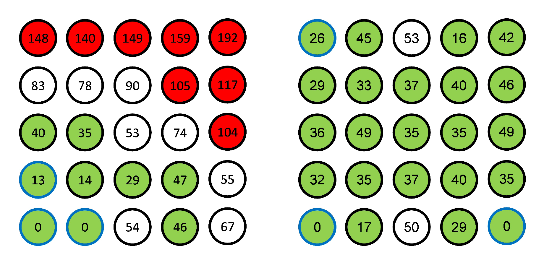
The accuracy increases with the CSY distance up to 600 mm and slightly decreases for the largest size. The length of the CSY determines the scale that is applied to the point cloud, so when using the 200 mm CSY, this length is multiplied by 4 to calculate the scale at the 800 mm points. Therefore any error in locating the 200 mm points will also multiply and have a large effect on the scaling of the grid. When using the 800 mm CSY, there is no scaling up of any errors, making these CSY points more accurate. The decrease in accuracy seen past 600 mm is due to the 800 mm spheres being at the corners of the sphere grid. These corner points are not as accurate as those closer to the center as the camera is focused at the center of the grid. Additionally, there is a larger camera lens distortion towards the outside of the field of view, where the corner points are located. This point quality is shown by the photogrammetry software RMS residual and is shown in Figure 5. Each circle represents one of the spheres in its corresponding position in the 5 × 5 grid, contained within is the RMS residual in pixels. Highlighted in red are those spheres with residuals greater than 0.1 pixels and in green are those less than 0.05 pixels, showing the greater quality toward the center.

Placing a 200 mm CSY at the centre produced an RMS accuracy of 36 $\mathsf{\mu }\mathrm{m}$ and a 400 mm CSY placed at the centre produced a 30 $\mathsf{\mu }\mathrm{m}$ RMS accuracy. Based on these findings, the ideal position for the scale bar would be in the center of the image where the points have the highest accuracy. However, this is not practical for use on the large mirrors as there is no suitable mounting point in the center of the glass for any externally used scaling artifact.

Figure 6 shows the individual sphere errors across the 5 × 5 grid for the 200 mm CSY and the 800 mm CSY. Highlighted in red are those points with an error greater than 100 $\mathsf{\mu }\mathrm{m}$ and in green are those less than 50 $\mathsf{\mu }\mathrm{m}$. It is clear that when the smaller CSY is used, there is a large error at the opposite corner, whereas with the large CSY the error is reduced and evenly distributed. The spheres used as CSY points are outlined in blue. The measurements were done using the previously found camera settings and parameters of aperture $f/7.1$, shutter speed $1/125$ $\mathrm{s}$, target size 10 mm, eight photograph positions with two roll angles at each. The results show that the accuracy of the photogrammetry measurement points is $40.8$ $\mathsf{\mu }\mathrm{m}$ RMS with a standard deviation of $0.3$ $\mathsf{\mu }\mathrm{m}$ over the 800 mm square grid. Such accuracy is well within the defined requirement for measuring the parabolic mirrors. It is clear from these results that a coordinate system should be set up using points separated as much as possible. Such points should be placed at the corners of the mirrors, or the corners themselves identified and used.

A comparison was made between the measurements both with and without camera calibration, and the results are shown in Figure 7 demonstrate the importance of the effect of camera calibration on the error map. The RMS difference is $12.1$ $\mathsf{\mu }\mathrm{m}$ for the $(x,y)$ position, which is at the level of accuracy of photogrammetry. This reinforces the result shown by the sphere targets measurements that it is therefore key to carefully consider the camera calibrations as they may cause systematic features in the error maps which are not an accurate representation of the surface.

3.2. Facet Measurements

Figure 8 shows the high-resolution CMM error map, measured with a point spacing of 20 mm in x and y. This shows clearly the effect of the ribbed structure in the central vertical line and the variations around the support points.

Figure 9a shows a close-up of the top left corner of Figure 8, clearly showing the effect of the supporting rib structure on the shape of the mirror. Figure 9b shows the results of an edge detection algorithm which displays more clearly the contours of the effect of the structure. The magnitudes of these variations are of the order of 50$\mathsf{\mu }\mathrm{m}$ to 100 $\mathsf{\mu }\mathrm{m}$ in height with a length of approximately 50 mm to 100 mm, which are small when compared to the millimeter-scale distortions expected and so are likely not to be seen. They are also of the order of the accuracy of photogrammetry and would require a very dense target grid in order to be seen. As a result of these measurements, a point spacing of 50 mm was used for subsequent CMM measurements.

Eight repeat measurements of the mirror facet were taken with the CMM, and the averaged result is shown in Figure 10. The RMS repeatability of the z values is $1.2$ $\mathsf{\mu }\mathrm{m}$.

These measurements were done with the target sheets already attached to the mirror surface. The thickness of the target sheets was 100 $\mathsf{\mu }\mathrm{m}$, and its compressive flexibility contributes to the increased variation in successive measurements, over the expected sub-micron level for the CMM. The x and y repeatability can be seen in Figure 11, with RMS values of $0.3$ $\mathsf{\mu }\mathrm{m}$ and $0.8$ $\mathsf{\mu }\mathrm{m}$ respectively, at the expected level for the CMM.

Figure 12 shows the error map produced from the averaging over the 8 CMM measurements calculated as the departure from the ideal parabolic equation. The map is formed from a 23 × 26 grid with 50 mm spacing in x and 60 mm in y. The two anomalous points seen in Figure 10 appear here as raised points, again indicating that these are caused by bubbling, which can be seen on further inspection as distortions in the elliptical appearance of the targets (as shown in Figure 13).

Photogrammetry measurements were repeated 10 times on the undistorted mirror. Figure 14a–c show the standard deviations in the x, y and z-directions respectively. The maximum variation occurs at the corners at 40 $\mathsf{\mu }\mathrm{m}$ with the overall RMS deviation at $9.3$ $\mathsf{\mu }\mathrm{m}$. Each directional repeatability map shows higher variations away from the central area of the mirror, as does the vector deviation map (Figure 14d), defined such that $S{D}^2=S{X}^2+S{Y}^2+S{Z}^2$. The z deviations are much lower than those seen in the x and y directions. The variation seen moving away from the central area are most likely due to the lower residual present nearer the focal position of the camera and towards the central area of the lens, where the points are generally better.

The averaged photogrammetry error map is shown in Figure 15 This error map is clearly curved in the y-direction, indicating an overall focal error on the mirror, shown in Figure 16. The peak-valley error is $1.4$ mm, with an RMS value of $0.44$ mm overall.

If the focal length is allowed to vary in the fitting algorithm, this curve error is removed, and the underlying waviness is revealed in more detail, as shown in Figure 17. The high points which remain are in the positions of the four corner support points and are due to the weight of the mirror. The peak–valley error is now $0.9$ mm, with an RMS of $0.16$ mm.

3.3. Photogrammetry Validation

The photogrammetry and CMM results are compared against each other by using the generated error maps, which are averages over 10 repeats themselves. Due to the different positions and densities of measured points, each point cloud was interpolated to the same set of x and y coordinates. So as to only perform this interpolation once, the photogrammetry surface map is interpolated to the CMM x and y values. The corresponding z values are then subtracted with the result shown in Figure 18.

The peak to valley correlation is $0.4$ mm, with an RMS of 76 $\mathsf{\mu }\mathrm{m}$. There are a number of anomalous points that appear as either red or dark blue. These are likely caused by bubbles, where the photogrammetry and CMM results may differ by compression of the bubble by the probe. A bubble may also cause a distortion in the viewed target, which may cause the software to calculate its position incorrectly. Each point was identified using its unique coded number, checked on the mirror itself and then excluded from further calculations. The correlation is 20 times less than the peak–valley value observed in the form error maps, and 5.7 times less than the RMS value. There is some pattern in the correlation map, particularly some horizontal striping and a slight vertical variation. There is no radial dependence visible, which shows that the camera calibration was successful.

The local slope in the curved direction at each measured point was calculated from the photogrammetry point cloud data by interpolation between neighboring points. The deviation of this measured slope from the ideal slope calculated from the parabolic equation was then found to produce a slope error map for the photogrammetry measurement, which is shown in Figure 19.

The peak to valley slope error is 12 mrad, with an RMS of 2.7 mrad. The largest slope errors occur at the top and bottom of the mirror and are due to the incorrect focal length seen in Figure 20. This slope error causes defocus, and it is in these regions that most of the mirror efficiency would be lost.

Performing a ray trace by using the calculated slopes of the point cloud produces the images shown in Figure 20. The inset figure details the absorber tube ideal location and shows both the inner steel and outer glass tubes. All the light rays appear to hit the steel tube, with a 100% intercept factor, but there is a clear difference in the focal position from the center of the tube.

3.4. Onsite Measurements

A measurement campaign was performed at the MATS plant, Borg El Arab, Egypt. At the time of measurement, this plant was in the installation phase and photogrammetry was used to qualify the mirrors. The mirrors were of the same type previously used for laboratory validation.

Measurements were done on four single facets, three outer facets and one inner facet across three collector modules in the same row. The facets measured are detailed in Figure 21. Mirror 1 is located on module 4, and its position is shown in red, mirror 2 is located on module 3 and is in the same position as mirror 1 (red). Mirrors 3 and 4 are located on module 4 and are shown in blue and green respectively.

The facets were washed, dried, and photogrammetry target sheets with 10 mm diameter targets were attached to the surface. Additional targets were placed at the corners of the facets as reference points. The targets attached to the facet can be seen in Figure 22.

Between 20 and 30 photographs were then taken from different positions around the facets and processed using the PhotoModeler software. The point cloud was imported into MATLAB and the parabolic equation $z=y^2/4F$ with a focal length F of $1.81$ $\mathrm{m}$ was fitted. The surface error map for each measurement was calculated by comparing the actual point position to the ideal surface. The point cloud was then interpolated to a 35 × 35 point grid to calculate the slope at each point. This was compared to the slopes of the ideal surface, and slope error maps were determined. The slope was then used in a ray-tracing algorithm to predict the path of light reflecting from the mirror towards the receiver tube. The distance of closest approach between the reflected light ray and the center of the ideally placed receiver was calculated as the defocus distance. The intercept factor was determined by counting the percentage of light rays with a defocus distance greater than the radius of the inner receiver tube.

Outer mirrors 1, 2 and 3 had three repeat measurements each, and inner mirror 4 had two repeat measurements. The results of one of these measurements are shown in Figure 23 below. The surface error map (Figure 23a) shows the departure from the ideal shape. The slope error (Figure 23b) was calculated by comparing the slope of the measured shape to the slope from the parabolic equation. The ray trace (Figure 23c) was calculated using the slope of the measured shape. This ray trace includes the design position of the receiver tube, which was not measured. From this ray trace, the intercept factors were calculated including the shape of the sun, taken as a Gaussian with width 2.73 mrad. The variation of the intercept factor over the facet is shown in Figure 23d. Finally the values for the RMS surface error, the RMS slope error, the RMS defocus (the distance away of each ray from the center of the tube), and RMS intercept factors were calculated.

The results show an average intercept factor of 92.5% for mirror 1, 85.6% for mirror 2, 92.0% for mirror 3 and 94.9% for mirror 4. The overall intercept factor across all mirrors is 91.3%. The detailed results for all measurements are shown in

Table 3. Photogrammetry measurement results.

Name	RMS Form (mm)	RMS Slope (mrad)	RMS Defocus (mm)	Intercept Factor (%)
Mirror1-1	1.20	2.35	17.2	94.6
Mirror1-2	1.15	2.94	19.5	91.5
Mirror1-3	1.14	2.85	19.3	91.5
Average	1.16	2.71	18.7	92.5
Mirror2-1	1.29	3.35	21.3	89.3
Mirror2-2	1.39	4.36	25.9	81.9
Mirror2-3	1.35	3.83	23.7	85.7
Average	1.34	3.84	23.7	85.6
Mirror3-1	0.98	2.46	17.9	93.4
Mirror3-2	1.15	2.84	19.5	91.4
Mirror3-3	1.10	2.92	19.6	91.1
Average	1.08	2.74	19.0	92.0
Mirror4-1	0.59	3.48	16.5	95.5
Mirror4-2	1.20	3.79	17.3	94.4
Average	0.90	3.64	16.9	94.9
Overall Average	1.12	3.23	19.6	91.3

.

4. Conclusions

A photogrammetry capability was developed using a Canon 600D DSLR camera and static cling vinyl sheet targets. The camera settings optimized were the aperture and the shutter speed, with camera positioning and the number of photographs taken also investigated. Although photogrammetry has been previously used by several R&D centers for measuring solar concentrators, the experimental optimization of camera settings, along with their influence on the measurement accuracy have not been previously well defined. A large coordinate measuring machine, traceable to international standards, was used to validate the developed photogrammetry technique, showing a correlation between photogrammetry and the CMM of 76 $\mathsf{\mu }\mathrm{m}$ RMS over the whole mirror facet. Measurements of mirror form showed errors of $0.4$ mm RMS with a peak to valley value of $1.4$ mm. The determined accuracy of photogrammetry is therefore sufficient to be able to measure the errors of such mirrors, magnitudes of which may typically be in excess of 3 mm. The technique was applied to installed mirrors at a CSP plant and the results were used to qualify the mirror installation. The errors found during the site measurements were of the order of 1 mm RMS with intercept factors in excess of 92%. One mirror was identified with a lower intercept factor of 85% indicating required adjustment. Subsequent improvements to the technique, which are currently being investigated, include the use of an aerial platform for measurement. An aerial platform, for example, a multi-rotor drone, would enable faster measurements of whole collector fields. This kind of platform is already being developed for deflectometry by Prahl et al. [22]. Additional developments may include the use of advanced image processing, for example through neural networks, to identify key features and edges that may be used to improve the bundle adjustments. This could be used in faceted mirror fields in place of some targets.

References

1. Gee, R.; Brost, R.; Zhu, G.; Jorgensen, G. An improved method for characterizing reflector specularity for Parabolic Trough Concentrators. In Proceedings of the SolarPACES 2010, Perpignan, France, 21–24 September 2010. [Google Scholar]
2. Shortis, M.R.; Johnston, G.H.G.; Pottler, K.; Lüpfert, E.; Commission, V. Photogrammetric Analysis of Solar Collectors. Int. Arch. Photogramm. Remote Sens. Spat. Inf. Sci. 2008, 37, 81–88. [Google Scholar]
3. Sansom, C.; Comley, P.; Bhattacharyya, D.; Macerol, N. A Comparison of Polymer Film and Glass Collectors for Concentrating Solar Power. Energy Procedia 2014, 49, 209–219. [Google Scholar] [CrossRef] [Green Version]
4. Forman, P.; Müller, S.; Ahrens, M.; Schnell, J.; Mark, P.; Höffer, R.; Hennecke, K.; Krüger, J. Light concrete shells for parabolic trough collectors—Conceptual design, prototype and proof of accuracy. Sol. Energy 2015, 111, 364–377. [Google Scholar] [CrossRef]
5. Huang, W.; Han, Z. Theoretical analysis of error transfer from the surface slope to the reflected ray and their application in the solar concentrated collector. Sol. Energy 2012, 86, 2592–2599. [Google Scholar] [CrossRef]
6. März, T.; Prahl, C.; Ulmer, S.; Wilbert, S.; Weber, C. Validation of Two Optical Measurement Methods for the Qualification of the Shape Accuracy of Mirror Panels for Concentrating Solar Systems. J. Sol. Energy Eng. 2011, 133, 031022. [Google Scholar] [CrossRef]
7. Arancibia-Bulnes, C.A.; Peña-Cruz, M.I.; Mutuberría, A.; Díaz-Uribe, R.; Sánchez-González, M. A survey of methods for the evaluation of reflective solar concentrator optics. Renew. Sustain. Energy Rev. 2017, 69, 673–684. [Google Scholar] [CrossRef]
8. Peña-Cruz, M.I.; Arancibia-Bulnes, C.A.; Monreal Vidal, A.; Sánchez González, M. Improving parabolic trough mirror module qualification by FOCuS tool. J. Renew. Sustain. Energy 2014, 6, 013118. [Google Scholar] [CrossRef]
9. Andraka, C.E.; Yellowhair, J.; Trapeznikov, K.; Carlson, J.; Myer, B.; Stone, B.; Hunt, K. AIMFAST: An alignment tool based on fringe reflection methods applied to dish concentrators. J. Sol. Energy Eng. Trans. ASME 2011, 133, 1–6. [Google Scholar] [CrossRef] [Green Version]
10. Zhao, W. Testing an aspheric mirror based on phase measuring deflectometry. Opt. Eng. 2009, 48, 103603. [Google Scholar] [CrossRef]
11. Diver, R.B.; Moss, T.A. Practical Field Alignment of Parabolic Trough Solar Concentrators. J. Sol. Energy Eng. 2007, 129, 153. [Google Scholar] [CrossRef]
12. Wendelin, T.J.; May, K.; Gee, R. Video Scanning Hartmann Optical Testing of State-of- the-Art Parabolic Trough Concentrators. In Proceedings of the Solar 2006 Conference, Golden, CO, USA, 7–13 July 2006. [Google Scholar]
13. Burgess, G.; Shortis, M.; Kearton, A.; Garzoli, K. Photogrammetry for dish concentrator construction. In Proceedings of the 47th ANZSES Annual Conference, Solar09, Townsville, Australia, 29 September–2 October 2009. [Google Scholar]
14. Jones, T.W.; Pappa, R.S. Dot Projection Photogrammetric Technique for Shape Measurements of Aerospace Test Articles. In Proceedings of the 40th AIAA Applied Aerodynamics Conference, Reno, NV, USA, 14–17 January 2002. [Google Scholar]
15. Weber, C.; Ulmer, S.; Koch, H. Enhancements in high-resolution slope deviation measurement of solar concentrator mirrors. Energy Procedia 2014, 49, 2231–2240. [Google Scholar] [CrossRef] [Green Version]
16. García-Cortés, S.; Bello-García, A.; Ordóñez, C. Estimating intercept factor of a parabolic solar trough collector with new supporting structure using off-the-shelf photogrammetric equipment. Appl. Energy 2012, 92, 815–821. [Google Scholar] [CrossRef]
17. Shortis, M.; Clarke, T.; Short, T. A comparison of some techniques for the subpixel location of discrete target images. In Proceedings of the Videomatrics III SPIE, Boston, MA, USA, 6 October 1994; Volume 2350, pp. 239–250. [Google Scholar]
18. De Asís López, F.; García-Cortés, S.; Roca-Pardiñas, J.; Ordóñez, C. Geometric optimization of trough collectors using terrestrial laser scanning: Feasibility analysis using a new statistical assessment method. Meas. J. Int. Meas. Confed. 2014, 47, 92–99. [Google Scholar] [CrossRef]
19. Shortis, M.R.; Johnston, G.H.G. Photogrammetry: An Available Surface Characterization Tool for Solar Concentrators, Part I: Measurements of Surfaces. J. Sol. Energy Eng. 1996, 118, 146. [Google Scholar] [CrossRef]
20. Skouri, S.; Ben Haj Ali, A.; Bouadila, S.; Ben Nasrallah, S. Optical qualification of a solar parabolic concentrator using photogrammetry technique. Energy 2015, 90, 403–416. [Google Scholar] [CrossRef]
21. Ydrissi, M.E.; Ghennioui, H.; Bennouna, E.G.; Farid, A. Geometric, optical and thermal analysis for solar parabolic trough concentrator efficiency improvement using the Photogrammetry technique under semi-arid climate. Energy Procedia 2019, 157, 1050–1060. [Google Scholar] [CrossRef]
22. Prahl, C.; Röger, M.; Hilgert, C. Air-borne shape measurement of parabolic trough collector fields. AIP Conf. Proc. 2017, 1850. [Google Scholar] [CrossRef]
Figure 1. Parabolic trough facets on coordinate measuring machine (CMM).
Sustainability 12 00196 g001
Figure 2. Flowchart of the validation process.
Sustainability 12 00196 g002
Figure 3. Flowchart of the general photogrammetry analysis process.
Sustainability 12 00196 g003
Figure 4. Camera angles.
Sustainability 12 00196 g004
Figure 5. Root mean square (RMS) residuals over sphere grid (in pixels).
Sustainability 12 00196 g005
Figure 6. Sphere errors in μm between photogrammetry/CMM for a 200 mm CSY (l) and 800 mm CSY (r).
Sustainability 12 00196 g006
Figure 7. Camera calibration effects.
Sustainability 12 00196 g007
Figure 8. High-resolution CMM error map.
Sustainability 12 00196 g008
Figure 9. Close up of high-resolution CMM map.
Sustainability 12 00196 g009
Figure 10. CMM repeatability in z (mm).
Sustainability 12 00196 g010
Figure 11. Repeatability in x (a) and y (b) directions (mm).
Sustainability 12 00196 g011
Figure 12. CMM error map.
Sustainability 12 00196 g012
Figure 13. Target sheet bubbles.
Sustainability 12 00196 g013
Figure 14. On CMM repeatability.
Sustainability 12 00196 g014
Figure 15. Photogrammetry form error map.
Sustainability 12 00196 g015
Figure 16. Form error.
Sustainability 12 00196 g016
Figure 17. Photogrammetry error map—form removed.
Sustainability 12 00196 g017
Figure 18. Correlation between CMM and photogrammetry.
Sustainability 12 00196 g018
Figure 19. Photogrammetry slope error.
Sustainability 12 00196 g019
Figure 20. Ray trace for photogrammetry.
Sustainability 12 00196 g020
Figure 21. Locations of measured facets.
Sustainability 12 00196 g021
Figure 22. Locations of measured facets.
Sustainability 12 00196 g022
Figure 23. Photogrammetry results for MATS measurements.
Sustainability 12 00196 g023