Reviewing Arch-Dams’ Building Risk Reduction Through a Sustainability–Safety Management Approach

Abstract

The importance of dams is rapidly increasing due to the impact of climate change on increasing hydrological process variability and on water planning and management need. This study tackles a review for the concrete arch-dams’ design process, from a dual sustainability/safety management approach. Sustainability is evaluated through a design optimization for dams´ stability and deformation analysis; safety is directly related to the reduction and consequences of failure risk. For that, several scenarios about stability and deformation, identifying desirable and undesirable actions, were estimated. More than 100 specific parameters regarding dam-reservoir-foundation-sediments system and their interactions have been collected. Also, a summary of mathematical modelling was made, and more than 100 references were summarized. The following consecutive steps, required to design engineering (why act?), maintenance (when to act) and operations activities (how to act), were evaluated: individuation of hazards, definition of failure potential and estimation of consequences (harm to people, assets and environment). Results are shown in terms of calculated data and relations: the area to model the dam–foundation interaction is around 3.0 H_d², the system-damping ratio and vibration period is 8.5% and 0.39 s. Also, maximum elastic and elasto-plastic displacements are ~0.10–0.20 m. The failure probability for stability is 34%, whereas for deformation it is 29%.

1. Introduction

There are many factors, largely controlled by the structures size, that hinder sustainability in the field of dam engineering. In this sense, the height of the blocks can reach more than 100 m and the crown length can reach more than 500 m [1,2]. Dams with these dimensions are called “super-high dams” [3,4]. Then, the presence of structural elements [5], and their interactions, with different functions that increase the difficulty of calculation and modelling, e.g., the cantilevers that support and distribute the vertical loads and the arches that distribute the horizontal loads. Finally, the interaction of dam, foundation, sediments and reservoir sub-systems, requires not only the knowledge of the structural and hydraulic engineering, but also, other engineering areas are involved.

Three aspects, namely geometry, behaviour, and materials, comprise the internal and intrinsic actions, which exclude the external actions and their uncertainties of probability and occurrence. These uncertainties are called “random” and are related to the magnitude of variability and inherent randomness. Besides these types of uncertainties, there are the “epistemic” uncertainties that are related to the lack of knowledge of materials and models [6]. Random and epistemic uncertainties are studied in stochastic analyses, which are used to solve problems that cannot be deterministically solved because models are not known, or data are not available.

Due to the doubts of the input data, analyses, methodologies, and results, the concept of “risk” and quantitative risk assessment (QRA) is introduced through the following equation:

Risk = ∫[P(L,E) × P(R|L) × C(L,R)]

(1)

where L = loads, E = events, and R = responses. P[R|L] is the conditional probability that R is true, given that L is true, and C stands for the consequences [7,8].

This integral is a measure of risk quantification based on the occurrence and probability of L, E and R, regarding the variability of extreme events, e.g., flooding, hurricanes, earthquakes, explosions. The interest of the concrete arch-dams is proven by the fact that several studies have been published since 1931 [9]. This interest has generated several codes/manuals/reports [10,11,12,13,14]. Furthermore, several academic works with the following goal have been published. First, there are researches about the definition of the shape (volume and area of concrete) optimization, aimed to minimize the cost and the impact of the dam body on the environment [15,16,17,18,19,20,21,22,23]. Then, publications addressing the analysis of the dam behaviour under seismic actions accounting the enormous importance of the structure [24,25,26,27,28,29,30,31,32,33]. Finally, there are studies that consider the fact that the dam body is linked with the foundation base, water reservoir, and soil sediments [34,35,36,37,38,39].

However, there are some aspects, described as follows, that are not well studied either synthetized or published in the literature. In this sense, the response estimation of arch-dams are not well studied or categorized, for example the effects of the non-uniform temperature variation due to the solar radiation and convective heat [30,40,41,42,43,44]. Furthermore, a good calibration between the theoretical and practical data is often difficult to obtain. In this sense, there is a lack of experimental tests made in the laboratory, which allow verifying the analytical and computational models. Also, there is a lack of practical experience of researchers and technical engineers do not easily accept the insights of researchers. In this sense, some cases about real concrete arch-dams are listed in Appendix A (see

Table A1. Some cases of real concrete-arch dams studied for scientific purposes.

Dam Name	Location	Researched Main Topics	Reference
Ertan Dam	Sichuan province, Southwestern China	Modal analysis. Seismic response	[84]
Tsankov Kamak Dam	Vacha River, Southwestern Bulgaria	Monitoring. Dam performance	[85]
Longyangxia Dam	Qinghai province, China	Dam-water-foundation interaction. Shock wave effects	[86]
Ridracoli Dam	Emilia Romagna, Italy	Modelling and reconstruction of dams. Unmanned aerial vehicle (UAV) photogrammetry	[54]
Lancang River Dam	Yunnan, China	Optimal sensor placement. Monitoring	[87]
Outardes 3 Dam	Quebec, Canada	Dam-reservoir-foundation interaction. Seismic analysis	[38]
Brezina Dam	Beyadh, Algeria west	Dam-water-foundation interaction. Sloshing effect	[35]
Shapai Dam	Sichuan province, China	Dam hazards. Seismic performance	[67]
Morrow Point Dam	Southwest Denver, Colorado	Shape optimal design. Fluid-structure interaction	[88]
Xiluodu Dam	Sichuan province, China	Excavation optimization design. Stability analysis	[89]
Rules Dam	Granada, Southern Spain	Probabilistic and deterministic seismic hazard. Dynamic analysis	[48]
Dagangshan Dam	Southwest China	Seismic damage. Joint opening. Artificial accelerograms	[26]
Jinping I Dam	Sichuan Province, China	Permeability of foundations. Behaviour of transient groundwater flow	[90]
Cabril Dam	Castelo Branco, Portugal	Seismic performance. Hydrodynamic pressures respect to the water level	[91]

). Finally, but not least, there is a clear lack of academic papers that synthetize, integrate, and summarize most of the aspects involved in sustainability of concrete arch dam building. This review paper mainly aims to cover this deficiency, which comprises its main novelty too. This is performed herein by reviewing the existent knowledge on the development of sustainability and safety assessment through the study of structural stabilities/deformations and failure risk, respectively.

The rest of this paper is organized as follows: Section 2 shows a background about the data and mathematical modelling. Section 3 describes some main key findings about an operating system and the project variables in a managerial context [7,12,14]. Section 4 is dedicated to the materials and methodologies followed in this research, describing the structure gand content of the different stages. Regarding materials, Random Variables (RVs) are showed; on the other hand, methods such as Monte Carlo Simulation (MCS), sustainability assessment framework and seismic hazard assessment are described. Then, Section 5 comprises the description of results, largely addressing the sustainability assessment of structural stability and deformations. Finally, Section 6 is dedicated to show the main conclusions drawn from this research.

2. Data and Mathematical Modelling Background

The case study is the Rules Dam, which is situated on the Guadalfeo River in the Granada province, Southern Spain. It is a super-high concrete arch-gravity, formed by 32 blocks, with single curvature, 509 m of crown length and maximum height of the vertical cantilever H_d 132 m. The Down-Stream (DS) and Up-Stream (US) slope faces are 1:0.60 and 1:0.18, respectively. The capacity and area for the maximum operating level H_o,r (i.e., water depth of 113 m) of the reservoir are 117.07 Hm³ and 308 Ha, respectively. The area of the water basin is 1070 km² [1,2].

The whole system of concrete arch-gravity dams is composed by four sub-systems, i.e., dam, foundation, reservoir and sediments. Usually, only the dam-reservoir-foundation system is studied, and, in many analyses, sediments are not considered as a separated system, but they are included in the reservoir or foundation sub-system. The parameters of the sediments as well as the foundation are very complicated to estimate, unless specific analyses “in situ” are developed. Moreover, it is very complicated to model them because they are not visible without adequate means.

Considering the precedent studies of the authors about the dam [45,46,47,48,49], more of 100 technical data regarding the system dam-reservoir-foundation-sediments have been summarized and shown in the Appendix A (see

Table A2. Collected data relative to dam sub-system.

Dam
Geometry		Material (Concrete)		Behaviour (Solid: Elasto-Plastic)
Blocks number [83]	32	Density ρd (kN/m3) [92]	24	T1,d (s) [48]	0.284
US slope [83]	0.18	Volume (103 m3) [83]	2051	T2,d (s) [48]	0.245
DS slope [83]	0.6	fcd (MPa) [47]	47.5	T3,d (s) [48]	0.208
Base’s max. length (m)	102 *	fcm (MPa) [92]	58	MPMR for T1,d in x, y, x (%) [48]	45.1
Crown length (m)	10 *	σc (MPa)	38.46*	Mass (106 kg)	4830 *
Crown height (m)	7.5 *	Ecm (GPa) [47]	44.4	Stiffness (GN/m)	2406 *
Crown long. length (m) [83]	509	Eep (GPa)	35.52*	Eq. inertia (m4)	1,376,852 *
Max. height Hd (m) [83]	132	εc1 (‰) [92]	2.45	Damping ratio ξd (%) [48]	5.0
Radius (m) [83]	500	εc (‰)	3.45 *	Blocks’ eq. mean period (s)	0.262 *
Ange in plane (°)	71 *	Ductility (= εc/εc1)	1.408	Blocks’ mean mass (106 kg)	130.56 *
Volume (103 m3)	2291 *	Thermal expansion (10−6 1/K) [92]	10	Blocks’ mean eq. stiffness (MN/m)	75,089 *
Voids’ volume (103 m3)	239 *	νd [47]	0.19	Blocks’ mean eq. inertia (m4)	43,027 *
Long. area (103 m2)	46 *	fctd (MPa) [47]	2.73	Concrete crack model
Spillway’s length (m) [83]	16.54	Gd (GPa)	9.92	εlt (‰) [47]	0.166
Min. block height (m)	7.0 *	cd (kN/m2) [63]	1000	ac (m) [47]	0.484
Blocks’ mean length (m) [83]	19.375	ϕd (°) [63]	55	wc (μm) [47]	240.51
Min. block volume (m3)	373 *			Gt (N/m) [47,93]	113.06
Max. block volume (103 m3)	125 *			h0 (m) [47,94]	1.35
Min. block long. area (m2)	137 *			lc (m) [47]	0.45
Max. block long. area (m2)	2463 *
Min. block trans. area (m2)	19 *
Max. block trans. area (m2)	6624 *

Note: * = Estimated value. US = Up-Stream. DS = Down-Stream. max. = Maximum. min. = Minimum. long. = Longitudinal. trans. = Transversal. f_cd = Design compressive strength. f_cm = Mean compressive strength at 28 days. σ_c = Compressive stress. E_cm = Secant modulus of elasticity. E_ep = Secant elasto-plastic modulus. ε_c1 = Strain at peak stress. ε_c = Shortening strain. ν_d = Poisson’s ratio of the concrete. f_ctd = Design tensile strength. G_d = Shear modulus. c_d = Cohesion of the concrete. ϕ_d = Angle of friction of the concrete. T_i,d = Structural period for i-th mode. MPMR = Modal participating mass ratios. eq. = Equivalent. ε_lt = Limit dynamic tensile strain. a_c = Effective crack length. w_c = Characteristic micro-crack opening that propagate through the aggregates. G_t = Tension specific fracture energy. h₀ = Size of the element that model l_c for the linear analysis. l_c = Crack band width of the fracture.

,

Table A3. Collected data relative to foundation sub-system.

Foundation
Material (Rock)		Behaviour (Solid: Elastic)
Density ρf (kN/m3) [48]	27.47	T1,f (s)	0.09 *
cf (kN/m2) [63]	45	Mass (103 kg)	205,175 *
ϕf (°) [63]	45	Stiffness (kN/m)	1.0 × 109 *
νf [47]	0.31	Damping ratio ξf (%)	10 *
Gf (GPa)	6.181 *	Geometry
Ef (GPa) [47]	41.55	Radius of semicircle (m2/m) [10]	27,355
Vs,f (m/s)	1500 *	Area (m2/m)	74,690 *
Eo,f (GPa)	109.34 *
Vp,f (m/s)	6309 *

Note: * = Estimated value. c_f = Cohesion of the foundation. ϕ_f = Angle of friction of the foundation. ν_f = Poisson’s ratio of the foundation. G_f = Shear modulus. E_f = Elastic modulus of foundation. V_s,f = Shear wave velocity in rock. V_p,f = Compressive wave velocity. E_o,f = Oedometric modulus. T_1,f = Foundation’s first period.

,

Table A4. Collected data relative to reservoir sub-system.

Reservoir
Geometry		Material (Water)
Operating level Ho,r (m) [48]	113	Density ρr (kN/m3) [49]	9.8
Operating level area (m2/m) [11]	38,307	Vp,r (m/s) [49]	1438
Flood level Hf,r (m)	120 *	Eb (GPa)	2.026 *
Flood level area (m2/m) [11]	43,200	Behaviour (Liquid: Viscous)
DS Operating level (m)	5.0 *	T1,r for Ho,r (m) [95]	0.314
Capacity for Ho,r (Hm3) [83]	117.07	T1,r for Hf,r (m) [95]	0.334
Area for Ho,r (Ha) [83]	308	Damping ratio ξr (%) [48]	0.5
Water basin area (km2) [83]	1070
Spillway capacity (m3/s) [83]	2987

Note: * = Estimated value. DS = Down-Stream. V_p,r (or C_r) = Compressive wave velocity. E_b = Bulk modulus of reservoir. T_1,r = Reservoir’s first period.

,

Table A5. Collected data relative to sediments sub-system.

Sediments
Material		Behaviour (Semi-Solid: Visco-Elastic)
Density ρs (kN/m3)	13 *	T1,s (s) [95]	0.014
cs (kN/m2)	20 *	Damping ratio ξs (%)	4.0 *
ϕs (°)	20 *	Geometry
νs	0.45 *	Area (m2/m) [11]	75.0
Gd,s (GPa)	0.81 *	Height Hs (m)	5.0 *
Ed,s (GPa)	0.27 *
Vs,s (m/s)	25 *
Vp,s (m/s)	1450 *
Eo,s (GPa)	2.73 *

Note: * = Estimated value. c_s = Cohesion of the sediments. ϕ_s = Angle of friction of the sediments. ν_s = Poisson’s ratio of the sediments. G_d,s = Shear modulus. E_d,s = Elastic modulus. V_s,s = Shear wave velocity in sediments. V_p,s = Compressive wave velocity in sediments. E_o,s = Oedometric modulus. T_1,r = Sediments’ first period.

,

Table A6. Parameters accounting the interactions.

Sub-Systems’ Combination	Parameter	Value
Dam + foundation + reservoir + sediments	Damping ratio (%) [48]	8.5
	Vibration period (s) [48]	0.393
Dam + foundation (rigid)	Impedance ratio	0.853 *
	Area (m2/m)	~ 3.0 Hd2 *
Dam + reservoir	Vibration period (s)	0.37*
Foundation + reservoir	q	5.655 × 10−5 *
	α [47]	0.85
Reservoir + sediments	q	5.199 × 10−4 *
	α	0.144 *

Note: * = Estimated value. q = Admittance coefficient. α = Wave reflection.

and

Table A7. Modelling types.

Model	Input	Output	Dimension	Description	Software
FEM [24,96]	Elements. Joints. Material properties. Loads	Stresses. Deformations. Modal parameters (e.g. frequency, modal participating mass ratio)	2D/3D	Discretization of an area or volume in mesh. A function is performed on each mesh and so the calculus is extended over the whole structure	[97]
Gravity method [29,98]	Loads. Geometry. Material properties	Stresses. Pressures. Stabilities	2D	It based on the rigid body equilibrium and beam theory. It performs stability analyses for hydrostatic loads and seismic loads	[50]
Numerical [47,99]	Differential equations. Boundary and initial conditions	Displacements. Velocities. Accelerations	2D/3D	By using interpolation function, it is possible to solve partial differential equations under specific conditions	[100]
Variational [90,101]	Functionals. Boundary and initial conditions	Optimum shape. Modal parameters (eigenvalues and eigenvectors)	2D	Through functionals, it is possible to find the maximum and minimum solutions	[100]
Analytical [95,102]	Analytical equations	Stresses. Pressures	1D	Substituting specific numerical values in the equations it is possible to find the solutions	[103]
BEM [19,53] a	Differential equations	Displacements. Velocities. Accelerations	2D/3D	It is a numerical computational method that solves partial differential equations under specific conditions	[64,65]
UAV photogrammetry [54,104]	Drones. Sensors	Geometry. Photogrammetry	3D	Geodetic survey of a study site by creating a detailed point cloud. It provides measurements from photographs	[105]
Geometric [9,106]	Measures. Quotes	Geometrical and architectural design	2D/3D	Plotting of drawings through heights, lengths and thicknesses	[107]
Experimental	Measures. Quotes. Tools. Laboratory	Simulations. Calibrations	3D	Reproduction of a structure with scaled dimensions respect to the real project	N/A
Rendering b	Measures. Quotes. Imagens	Photos. Animations	3D	Generation of 3D reconstructions by algorithms that define the colour and size of each point of the input image	[108]

Note: FEM = Finite Element Method. BEM = Boundary Element Method. UAV = Unmanned Aerial Vehicle. N/A = Not applicable. ^a Coupled BEM-FEM is used to study the fluid-structure interactions [19]. Also, accurate computation of fluid-structure nonlinear interaction is analysed by the immersed boundary method (IBM) proposed in [41]. ^b The reader can refer to specific bibliographies in the area of the design and/or architecture.

). The subscripts represent the four parts of the system, i.e., d = dam, f = foundation, r = reservoir, and s = sediments.

2.1. Dam Sub-System

Concrete arch-gravity dams are designed to be stabilized by equilibrium forces (horizontals and verticals). Each section of the dam must be stable and independent of any other section.

The dam body is formed by several arch and cantilever units. Arch refers to a portion of the dam bounded by two horizontal planes. Arches have uniform or variable thickness, i.e., the arches may be designed so that their thickness increases gradually on both sides of the reference plane. Cantilever is a portion of the dam contained between two vertical radial planes [10].

The function of arches is to distribute the horizontal stresses along the dam body, whereas the function of cantilevers is to transmit the vertical stresses from the top to the bottom. Moreover, the arch has an important role respect to the stiffness which increases on the dam body.

Dam sub-systems can be modelled using several theories and models that are briefly mentioned as follows.

• Rigid body equilibrium and beam theory. The gravity method is based: (1) on rigid body equilibrium to determine the internal forces acting on the potential failure plane (joints and concrete-rock interface), and (2) on beam theory to compute stresses. The use of the gravity method requires several simplified assumptions regarding the structural dam behaviour and loads application [50].
• Membrane theory (tank structures). The behaviour of arch-dams can be imagined as being similar to the behaviour of storage tanks: an arch in plant is a part of the tank circumference. The function of the elements is analogue, i.e., arch-dams are formed by cantilever and arch units, whereas tanks are formed by meridional and circumferential units. The stresses in the tanks are: vertical compressive stress (meridional compression associated with hydrostatic and hydrodynamic pressures) and tensile hoop stress (circumferential stress) [35,46,51,52].
• Independent blocks model. Here, the dam’s blocks are modelled as independent parts. Each block can be considered as a simple oscillator where the mass is the predominant parameter. This approximation is generally useful for estimating preliminary results [26,47].

Moreover, dam sub-systems can be modelled accounting the vertical joints, as follows.

• Monolithic model. The monolithic model ensures the continuity between adjacent blocks. The rigid connection between them is ensured by means of vertical joints, which are modelled by surface-based “tie” constraints that account the translational and rotational degrees of freedom [53,54,55]. Considering a series of monolithic, the model can be called “multi-monolithic model” [56].
• Surface-to-surface joints. The surface-to-surface joint model simulates the discontinuity between blocks along the contact surfaces. The contact model describes tangential and normal behaviour by adopting a coefficient of friction and contact pressures transmitted from surfaces [54,55].
• Solid elements joints. The solid element joint model simulates the joints, connected to the ashlars, as independent solid elements, separating the discontinuity surface and spacing the blocks. These joints are characterized by mechanical models (i.e., elastic or elasto-plastic model) [54,55].

2.2. Foundation Sub-System

Even if it is possible to analyse the four systems separately, it is too approximate to approach some aspects without considering the interactions. In this sense, the foundation sub-system is usually studied including the dam-foundation interactions.

The model that describes the dam base and top foundation contact is Mohr-Coulomb model. This model, used in the literature to evaluate base sliding [57], constitutes a simplified procedure to model a nonlinear single-degree-of-freedom system [58] and the failure mode under a reliability-based approach. This is performed as such due to the failure analysis of the dam–foundation interface being characterized by complexity, uncertainties on models and parameters, and a strong non-linear softening behaviour [59].

The foundation sub-systems can be modelled by a massed, massless, rigid, flexible model.

• The massed model (m ≠ 0, k = 0) is composed by finite elements that form the foundation [24]. In 3D analysis, it consists of solid elements, of which, each one is an eight-node element. It is based upon an isoparametric formulation that includes nine bending modes [40]. For each element the density of the material is assigned. The massed model only accounts the weight of the elements in static analysis and the inertial force in dynamic analysis.
• The massless model (m = 0, k ≠ 0) is composed by fixed joints (or nodal points). A joint is defined in three spatial coordinates x, y, z. It defines a joint individually, many joints on a line (or curve), surface or a three-dimensional region. The massless model accounts only material flexibility by elastic springs and forces. The foundation model should be extended to a large enough distance beyond which its effects on deflections and stresses of the dam become negligible [60]. It is possible to consider for the elastic modulus two cases: (i) the same modulus as the concrete and (ii) 1/5 the modulus of concrete [10].
• Rigid model (k → ∞). Rigid foundation model neglects dam-foundation interaction and, in fact, neither stiffness nor mass of the foundation is accounted in overall coupled equation of motion. It can be modelled by elastic springs with very high stiffness (e.g., ~ 1.0 × 10⁹ kN/m) or by fixed.
• The flexible model (k → 0), conceptually, it is equal to the massless model because it is formed by a series of joints where are applied springs. An order of magnitude of the elastic spring can be ~ 1.0 × 10⁶ kN/m.

2.3. Reservoir Sub-System

The main actions produced by water mass are the pressures, which can be static or dynamic pressures and act in horizontal or vertical directions. Reservoir sub-system can be approached by considering “rigid” or “flexible” dam, respectively. In this sense, it can be modelled as:

• Added mass, where the hydrodynamic pressures exerted on a dam, by an incompressible fluid, are considered [61]. The hydrodynamic pressures are the same as if a portion of the fluid body is forced to move back and forth with the dam and, that this “added mass” is confined in a volume bounded by a two-dimensional parabolic surface on the dam upstream side.
• Hydrodynamic interaction. Analytical equations for hydrodynamic response of dam-reservoirs considering compressibility effects during harmonic and arbitrary ground motions have been defined [62]. Effects of the deformability of the dam on hydrodynamic pressure have been introduced. The main limitation consists in considering the deformation by only the vibration fundamental mode of the structure [63].

A very popular modelling approach is the “acoustic elements”. This model simulates the pressure distributions of the fluid considering the compressibility of the fluid through the “bulk modulus”. To find a solution it is necessary to define appropriate boundary conditions, where the most important one takes place on the contact between fluid and structure [63,64,65]. Acoustic elements are used for modelling an acoustic medium undergoing small pressure changes. The solution in the acoustic medium is defined by a single pressure variable, which represents its degree of freedom [64,65].

2.4. Sediments Sub-System

Sediments can be modelled as a liquid (viscous model) or as a solid (elastic–plastic model). This is, because two cases should be considered: full and empty reservoir. In the first case, sediments are totally submerged, and therefore sediments can be considered in a more similar way to the liquid hydrodynamic behaviour. In contrast, in the second case, sediments can be dry (solid) or yet submerged (semi-solid) depending on the material of which sediments are made: if the predominant material is the sand soil, the liquid drains easily and thus sediments can be idealized as solid, whereas if it is made of clay soil, the liquid does not drain and so it can be idealized as a liquid.

Considering the two extreme cases, the liquid behaviour tends to the reservoir sub-system behaviour, whereas the solid tends to the foundation sub-system (liquid sediments → like reservoir sub system. Solid sediments → like foundation sub-system). The presence of sediments can affect the behaviour of the whole system. This is because, the reservoir bottom absorption affects the stiffness and damping ratio of the structure [34,66,67].

2.5. Interactions of Sub-Systems

By means of the aforementioned parameters of the four sub-systems, it is possible to define some parameters that account the interactions among sub-systems. By considering these values, it is possible to estimate some general relations that can be used to the design, for instance: (i) the area of rigid foundations under the dam can be estimated as ~ 3.0 H_d²; (ii) the contribution of the damping ratio of each sub-system respect to the damping ratio of the system is ξ_d = 0.05 (26%), ξ_f = 0.1 (51%), ξ_r = 0.005 (3%), ξ_s = 0.04 (20%); (iii) the contribution of the vibration period of each sub-system respect to the system vibration period is T_1,d (s) = 0.284 (40%), T_1,f = 0.09 (13%), T_1,r = 0.314 (45%), T_1,s = 0.014 (2%).

These percentages show the weight of each sub-system respect to the total response. However, it is important to note that these values refer to this specific case study or, more in general, to concrete arch-gravity dams under specific conditions.

Finally, a modelling process should be calibrated for accurately identifying the problem to be analysed. There is a closer correlation between models and types of analysis: The choice of a model (software) is based on the specific problem to be solved. Although nowadays, there are extremely complex models [68] that consider all the phenomena together, it is good to define and focus a specific problem aspect and then to converge and resolve it by using a unique model.

Each model is made to study a specific problem. It is important to consider all the parts of the whole system, but it is also necessary not to lose control of the parameters and their interactions.

3. Management Operating Systems

The managerial procedures that account for the risk analysis are studied in reliable papers [7,8,69] and guidelines [12,14]. Moreover, in the literature, it is possible to find several contributions regarding stability optimization for concrete arch-dams [17,18,22,36,45]. However, the search of a safety and no-safety domain by taking into account the stability and deformation of arch-dams in a managerial context, by considering some parameters (see

Table 1. Probabilistic parameters (collected results from [47,48,49]).

Parameter	Unit	Details	Mean RV	SD	CV (%) a	Distribution
Maximum dead stress	kN/m2	Stress at the heel dam (US face)	−2215.38	±221.54	10.0	N
Elastic displacement	mm	Top displacement of the central block	151.65	±30.33	20.0	N
Elasto-plastic displacement	mm	Top displacement of the central block	186.41	±37.28	20.0	N
Hydrostatic pressure	kN/m2	For Ho,r = 113 m	1107.40	±110.74	10.0	N
Hydrodynamic pressure	kN/m2	Pressures for flexible dam accounting compressible water. First three modes are considered.	350.55	±35.06	10.0	N
Acceleration	cm/s2	Horizontal PGA for a return period 1950 years	303.20	±60.64	20.0	N

Note: PGA = Peak Ground Acceleration. SD = Standard Deviation. N = Normal (Gaussian) distribution. ^a CV is the Coefficient of Variation defined by: CV = (SD/Mean RV) × 100.

later) obtained from several data, has not been carried out. In this sense, this paper provides a novelty for the research.

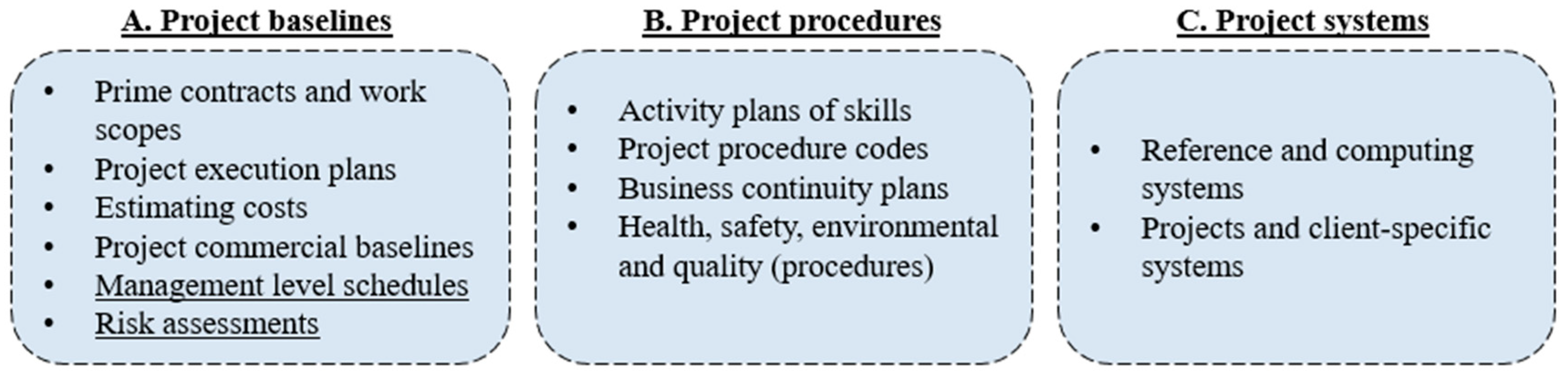
The project management is formed by design phases, which are called “project baselines”, “project procedures”, and “project systems”. Each phase contains several sub-phases listed in the Figure 1.

In this paper, a particular attention about the “management level schedules” and “risk assessment” is considered; the former estimates the possible scenarios, whereas the latter defines the hazards.

In analyses there are different parameters/values that usually are adopted: deterministic parameters (DP), probabilistic parameters (PP), semi-probabilistic parameters (SPP), semi-deterministic parameters (SDP) and super-probabilistic parameters (SP2). SPP are the parameters obtained by combining DP and PP, whereas SDP are obtained by DP and SPP. SP2 are obtained by a probabilistic analysis, which are recalculated and re-estimated using one or more probabilistic approaches. Deterministic parameters are usually well known through the literature (papers, books, codes, guidelines), experience (real projects, academic works, research projects), and empirical experimentation (laboratory work, building sites). Probabilistic parameters are not known, and therefore are subject to aleatory (inherent randomness) and epistemic (lack of knowledge of materials/models) uncertainties, as have already been introduced.

4. Materials and Methods

4.1. Materials

This research comprises the analysis of probabilistic approaches which are the most reliable and precise ones for analysing the stability of dams. In this sense, these analyses are based on the definition of probability density functions (PDFs) through several random variables (RVs). The parameters used to develop the analysis in this paper are listed in Table 1. These parameters come from precedent studies [47,48,49], and here are considered as RVs to carry out a sustainability assessment, and are therefore plotted by a probabilistic distribution with a mean and standard deviation (SD).

4.2. Methods

4.2.1. Monte Carlo Simulation (MCS)

To estimate possible scenarios, MCS, which generates RVs, has been used in following way. Limit State (LS) function G(X) is defined. When the domain G(X) < 0, the LS is called “no safety”, whereas when G(X) > 0, the LS is called “safety”. The separation of both domains is given when G(X) = 0 (limit domain). Given a random variable vector X = {x₁,…,x_j} = {x_i} for a LS function G(X) and f_X(x_i), which is the joint PDFs of x_i, the general probability x% that G(X) takes on a value less than 0 (called here probability of failure p_f) is [70,71]:

$${\mathrm{p}}_{\mathrm{f}}=\mathrm{P}\left[\mathrm{G}\left(\mathrm{X}\right)<0\right]={{\displaystyle \int }}_{\left\{\mathrm{X}:\mathrm{G}\left(\mathrm{X}\right)<0\right\}}{\mathrm{f}}_{\mathrm{X}}\left({\mathrm{x}}_1,\dots ,{\mathrm{x}}_{\mathrm{j}}\right){\mathrm{dx}}_1\dots {\mathrm{dx}}_{\mathrm{j}}={{\displaystyle \int }}_{\left\{\mathrm{X}:\mathrm{G}\left(\mathrm{X}\right)<0\right\}}{\mathrm{f}}_{\mathrm{X}}\left({\mathrm{x}}_{\mathrm{i}}\right){\mathrm{dx}}_{\mathrm{i}}$$

(2)

Equation (2) represents the cumulative failure probability (CFP), which represents the area of the PDF within a defined interval.

By using MCS, Equation (2) can be rewritten as:

$$p_f={{\displaystyle \int }}_{\left\{X: G\left(X\right)<0\right\}}I\left(x_i\right)f_X\left(x_i\right)d{x}_i$$

(3)

where I(∙) is an indicator function, defined by:

$$I\left(x_i\right)=\{\begin{array}{c}1, for G\left(X\right)\le 0\\ 0, for G\left(X\right)>0\end{array}$$

(4)

Finally, p_f can be considered as the mean value of I(x_i), i.e., Ī(x_i) = E[I(x_i)], therefore Equation (3) becomes:

$$p_f=\frac{1}{N}{{\displaystyle \sum }}_{i=1}^{N}I\left(x_i\right)=\frac{N_f}{N}$$

(5)

where N is the number of simulations (or samples) and N_f is the number of simulations with I(x_i) ≤ 0. It is note that the result of p_f is more accurate when N → ∞. In practice, samples required are 1 × 10^Nk where the choice of N_k is due to the computer power and available computational time.

4.2.2. Sustainability Assessment Framework

Sustainability has been assessed in this research from a double perspective. First, the perspective of temporal sustainability, closely related to the duration and useful life of arch dam infrastructures. This dimension is specifically articulated and assessed through the design parameters of “stability” and “deformation”. Secondly, sustainability has been assessed from a safety perspective articulated through risk calculation. Consequently, in a broad scale, sustainability assessment is developed from a dual sustainability/safety management approach (Figure 5). On the other hand, in a detailed scale, the sustainability of concrete arch dams is evaluated from a design optimization perspective, specifically, for dams´ stability and deformation. Additionally, the safety perspective is directly related to the reduction and consequences of failure risk. For this, several scenarios about stability and deformation, identifying desirable and undesirable actions, were estimated. Quantitative results on both dimensions of sustainability are provided and explained in results section.

There are several types of actions that are generated either by human or by nature. These actions can be catalogued as either “environmental actions” or “human actions”. All aspects regarding these actions are included in “impact matrices” where they are identified as “hazards”. Several hazards can affect the durability of structures, e.g., environmental, social and economic impact; population and consumptions growing; climate change (temperature and humidity) [72]; flooding; hurricanes; explosions of blast waves in the terrorist attacks [73] or in demolitions [74]; seismic hazard [75]; corrosion [76,77].

Here, the last two hazards are introduced since are known by authors. However, in this analysis only seismic hazard assessment is considered.

Structures are subjected to internal and external stresses and deformations due to (1) excitation of masses by seismic vibrations or general dynamic loading by extreme events, and (2) the corrosion of the reinforced concrete (RC) elements.

Table 2. Identification of impacting hazards.

Hazard	Approach	Scenarios
Seismic hazard	Poisson [49]. Bayesian [78]	Probability of occurrence
Corrosion	Diffusion [79]. Reliability [70]	Probability of failure

shows both hazards (as a succession: hazard → approach → scenarios), the relative approach and its scenario type.

Figure 2 shows the inter-combinations among the four sub-systems of the concrete arch-dams. It is possible to see all the possible combination among the dam-foundation, dam-sediments, dam-reservoir, foundation-sediments, foundation-reservoir and sediments-reservoir. By knowing the variables of the project, it is possible to treat the hazards in a practical way.

4.2.3. Seismic hazard assessment

The seismic events are extreme events that may be accurately studied. The seismic hazard is usually estimated by using two approaches: probabilistic and deterministic. The former, probabilistic seismic hazard analysis (PSHA) is based on the Cornell method [80] and Poisson distribution [71]. To apply it, it is necessary to know seismogenic zones, i.e., zones where the earthquakes are equally likely and independent of each other at any location (e.g., in Spain [81]).

The probability that a ground motion parameter S exceeds the ground motion level S₀ in i-th source area is defined by Λ_i, which depends on: the PDF of the magnitude f_m(m) and of the site-source distance f_r(r), the standardization Normal distribution f_ε(ε) [71] with the ground motion randomness ε and, the average annual rate of exceedance λ_c of an event with magnitude m described through the Gutenberg–Richter trend line [82], which provides the ratio between the number of small and large events and the level of seismicity [83].

The probability is defined by:

$${\Lambda }_i={\lambda }_c{{\displaystyle \int }}_m{{\displaystyle \int }}_r{{\displaystyle \int }}_{\epsilon }P\left[S>S_0|m,r,\epsilon \right]f_m\left(m\right)f_r\left(r\right)f_{\epsilon }\left(\epsilon \right)dm dr d\epsilon$$

(6)

If the analysis involves more of one seismogenic zones (where N_s = number of seismogenic zones), the probability of exceedance is defined by:

$${\Lambda }_{S_0}=P[S>S_0]={{\displaystyle \sum }}_{i=1}^{N_s}{\Lambda }_i$$

(7)

Figure 3 shows some curves (as results example) in terms of accelerations vs. structural period (Figure 3a) and hazard contribution respect to the magnitude and fault-site distance (Figure 3b).

MCS is used to analyse the sustainability of the structure respect to the stability and deformations. LS function is written as the difference between the stable actions A_s, and unstable actions A_u: G(X) = A_s(X) – A_u. When A_s < A_u, G(x) < 0, the failure is achieved.

Figure 4a,b shows the generated MCS points, whereas Figure 4c–d shows an example how to identify the LS function (Figure 4c) and the PDF in 3D (Figure 4d). To the left of the intersection point (Figure 4c), between stable and unstable trend line, there is the “no safety” state (G(X) < 0), whereas to the right of this point there is the “safety” state (G(X) > 0). The PDF in the (x_i, x_i+1) point represents the value of the probability around (x_i, x_i+1) point in relation to the amplitude of this around (density).

Figure 5 shows the methodology by the flow chart used in the analysis. The flow chart is divided in two principal parts: general and specific part. In the first one, the process and operation phase are defined. Here, choices, decisions, individuation of the structure (issue), hazards, and the possible approaches are established. Then, the technical actions are analysed in terms of data and control of modelling and analyses. Here, a specific concrete arch-dam is individuated (case study), by defining sub-systems data, RVs, methods and approaches (if the modelling and analysis are not satisfactory and are not consistent to the individuated hazards, it is necessary to start over). Finally, scenarios are estimated in terms of stability and deformations of the dam by providing safety and no-safety domain (sustainability assessment) and probability of failure (safety assessment). The flow chart concluded by taking a final decision from managers and technical engineers.

5. Results

5.1. Sustainability Assessment

Here, six scenarios to evaluate the sustainability assessment accounting the deformation and stability of concrete arch-dams are shown. Stable actions refer to the probabilistic parameters in Table 1. By knowing the mean RV and SD for each parameter it is possible to generate a several points by MCS.

To the left of the Figure 6 and Figure 7 the trend lines of the stable and unstable actions are shown. The horizontal dashed line indicates the LS line (i.e., the mean line when the stable line intersects the unstable line). For the stable action, its logarithmic trend line is also plotted, which shows better the progress of an action that starts from zero and reaches its maximum value. The logarithmic trend intersects the unstable line before respect to the linear stable trend. This gap could represent a security factor that increase the “safety” LS. When the dashed horizontal line rises, the p_f increases and so the “no safety” state is more probable.

To the right of the Figure 6 and Figure 7, the PDFs when (A_s = A_u) are plotted. The solid curves represent the PDFs by mean RVs, whereas the dashed curves represent the PDFs by negative SDs.

5.2. Safety Assessment

Finally, the risk management model defined in literature [12,14] show the need of defining the undesirable event with the potential for harm or damage in these following steps: individuation of hazards → defining of potential for failure → estimating of consequences (harm to people, assets, environment). These steps are needed to design and justify engineering activities (why act?), to propose activities maintenance (when to act) and to tackle operations activities (how to act).

In this sense, the safety management assessment can be evaluated by quantifying the p_f.

Table 3. Identification of impacting hazards.

Scenario	Parameter	Unit	Au	Mean of G(X)	SD of G(X)	pf
I	Dead stress	kN/m2	2130	85.4	128.33	0.3095
II	Elastic displacement	mm	140	11.32	17.40	0.3097
III	Elasto-plastic displacement	mm	170	16.71	21.67	0.2753
IV	Hydrostatic pressure	kN/m2	1065	42.52	63.65	0.3053
V	Hydrodynamic pressure	kN/m2	342	8.61	20.21	0.3791
VI	Acceleration	cm/s2	285	18.14	35.10	0.3496

and Figure 8 summarize the results in accordance to Figure 6 and Figure 7.

6. Summary

This paper mainly aimed to review the knowledge on the development of sustainability and safety assessment through the study of structural stabilities/deformations and failure risk consequences, respectively, for concrete gravity arch-dams.

In order to carry out the main analysis, several aspects have been defined: materials regarding the sub-systems (dam, foundation, reservoir, sediments) and their interactions; methods respecting to the operating systems of a project; deterministic and probabilistic variables; modelling and methodologies.

From precedent-specific studies of the authors investigating dam design, more than 10 theoretical modelling, 10 modelling types by software, more than 100 specific parameters, and more than 100 references are summarized.

This paper addresses and comprises critical aspects that are summarized as follows: (i) to show innovative approaches respecting to the enormous quantities of variables that are involved for concrete arch-dams; (ii) to provide numerical values of parameters to design concrete arch-dams; (iii) to show the project phases and methodologies; (iv) to estimate different scenarios respecting to the main actions on the dam system; (v) to contribute to the knowledge of the state-of-the-art about concrete arch dams.

The first results are shown in terms of new estimated data provided in the Appendix A. Other results concern the parameters of the interaction between dam–foundation–reservoir–sediments with respect to the area of rigid foundations under the dam (~ 3.0 H_d²), the contribution of each sub-system damping ratio respect to the system damping ratio (8.5%), and the contribution of each sub-system vibration period respect to the system vibration period (0.393 s). These values are useful to estimate some general relations that can be used to aid design. Moreover, the maximum elastic and elasto-plastic displacements are of the order of ~ 0.10–0.20 m that, in relation to the maximum dam height, is H_d/1000, in accordance with the literature [6].

Furthermore, the sustainability assessment demonstrates that the mean probability of failure of the stability of dam body and its deformation is about 32%. In particular, that for stability is 34%, which is higher than for the deformation at 29%. These mean percentages are quite large because unstable actions have been taken. When the intersection point between the stable and unstable line rises, the p_f increases, and so the “no safety” state is more probable. However, this raises the level of attention during the design of a monitoring method for concrete arch-dams, and in this sense, risk management can be carried out satisfactory.

References

1. Inventory of Dams and Reservoirs (SNCZI). Available online: http://sig.mapama.es/snczi/visor.html (accessed on 1 February 2019).
2. Spanish Association of Dams and Reservoirs (SEPREM). Available online: http://www.seprem.es/index.php (or: http://www.seprem.es/st_pe_f/JDFerrovial/PRESA_DE_RULES.pdf) (accessed on 1 February 2019).
3. Huang, H.; Chen, B.; Liu, C. Safety monitoring of a super-high dam using optimal kernel partial least squares. Math. Probl. Eng. 2015, 2015, 571594. [Google Scholar] [CrossRef] [Green Version]
4. Shi, Z.; Gu, C.; Qin, D. Variable-intercept panel model for deformation zoning of a super-high arch dam. SpringerPlus 2016, 5, 898–917. [Google Scholar] [CrossRef] [PubMed] [Green Version]
5. Zhang, Q.L.; Wang, F.; Gan, X.Q.; Li, B. A field investigation into penetration cracks close to dam-to-pier interfaces and numerical analysis. Eng. Fail. Anal. 2015, 57, 188–201. [Google Scholar] [CrossRef]
6. Hariri-Ardebili, M.A.; Saouma, V.E. Seismic fragility analysis of concrete dams: A state-of-the-art review. Eng. Struct. 2016, 128, 374–399. [Google Scholar] [CrossRef]
7. Hariri-Ardebili, M.A. Risk, reliability, resilience (R3) and beyond in dam engineering: A state-of-the-art review. Int. J. Disaster Risk Reduct. 2018, 31, 806–831. [Google Scholar] [CrossRef]
8. Altarejos-García, L.; Escuder-Bueno, I.; Serrano-Lombillo, A.; De Membrillera-Ortuño, M.G. Methodology for estimating the probability of failure by sliding in concrete gravity dams in the context of risk analysis. Struct. Saf. 2012, 36–37, 1–13. [Google Scholar]
9. Savage, J.L.; Houk, I.E. Checking arch dam design with models. Civ. Eng. 1931, 1, 695–699. [Google Scholar]
10. U.S. Army Corps of Engineers (USACE). Arch Dam Design, Manual No. 1110-2-2201; USACE: Washington, DC, USA, 1994. [Google Scholar]
11. U.S. Army Corps of Engineers (USACE). Theoretical Manual for Analysis of Arch Dams; Technical Report ITL-93-1; USACE: Washington, DC, USA, 1993. [Google Scholar]
12. International Commission on Large Dams (ICOLD). Selecting Seismic Parameters for Large Dams; Guidelines, Bulletin 148; ICOLD: Paris, France, 2016. [Google Scholar]
13. Federal Guidelines for Dam Safety (FEMA). Earthquake Analyses and Design of Dams; FEMA: Washington, DC, USA, 2005.
14. International Commission on Large Dams (ICOLD). Dam Safety Management: Operational Phases of the Dam Life Cycle; Bulletin 154; ICOLD: Paris, France, 2017. [Google Scholar]
15. Pouraminian, M.; Ghaemian, M. Multi-criteria optimization of concrete arch dams. Sci. Iran. 2017, 24, 1810–1820. [Google Scholar] [CrossRef] [Green Version]
16. Kaveh, A.; Ghaffarian, R. Shape optimization of arch dams with frequency constraints by enhanced charged system search algorithm and neural network. Int. J. Civ. Eng. 2015, 13, 102–111. [Google Scholar]
17. Seyedpoor, S.M.; Gholizadeh, S. Optimum shape design of arch dams by a combination of simultaneous perturbation stochastic approximation and genetic algorithm methods. Adv. Struct. Eng. 2008, 11, 500–510. [Google Scholar] [CrossRef]
18. Seyedpoor, S.M.; Salajegheh, J.; Salajegheh, E.; Gholizadeh, S. Optimal design of arch dams subjected to earthquake loading by a combination of simultaneous perturbation stochastic approximation and particle swarm algorithms. Appl. Soft Comput. 2011, 11, 39–48. [Google Scholar] [CrossRef]
19. Mahani, A.S.; Shojaee, S.; Salajegheh, E.; Khatibinia, M. Hybridizing two-stage meta-heuristic optimization model with weighted least squares support vector machine for optimal shape of double arch dams. Appl. Soft Comput. 2015, 27, 205–218. [Google Scholar] [CrossRef]
20. Zhang, X.F.; Li, S.Y.; Chen, Y.L. Optimization of geometric shape if Xiamen arch dam. Adv. Eng. Softw. 2009, 40, 105–109. [Google Scholar] [CrossRef]
21. Akbari, J.; Ahmadi, M.T.; Moharrami, H. Advances in concrete arch dams shape optimization. Appl. Math. Model. 2011, 35, 3316–3333. [Google Scholar] [CrossRef]
22. Shouyi, L.; Lujun, D.; Lijuan, Z.; Wei, Z. Optimization design of arch dam shape with modified complex method. Adv. Eng. Softw. 2009, 40, 804–808. [Google Scholar]
23. Gholizadeh, S.; Seyedpoor, S.M. Shape optimization of arch dams by metaheuristics and neural networks for frequency constraints. Sci. Iran. 2011, 18, 1020–1027. [Google Scholar] [CrossRef] [Green Version]
24. Mirzabozorg, H.; Varmazyari, M.; Ghaemian, M. Dam-reservoir-massed foundation system and travelling wave along reservoir bottom. Soil Dyn. Earthq. Eng. 2010, 30, 746–756. [Google Scholar] [CrossRef]
25. Lamea, M.; Mirzabozorg, H. Simulating structural responses of a generic AAR-affected arch dam considering seismic loading. Sci. Iran. 2018, 25, 2926–2937. [Google Scholar] [CrossRef] [Green Version]
26. Wang, J.T.; Jin, A.Y.; Du, X.L.; Wu, M.X. Scatter of dynamic response and damage of an arch dam subjected to artificial earthquake accelerograms. Soil Dyn. Earthq. Eng. 2016, 87, 93–100. [Google Scholar] [CrossRef]
27. Hariri-Ardebili, M.A.; Furgani, L.; Meghella, M.; Saouma, V.E. A new class of seismic damage and performance indices for arch dams via ETA method. Eng. Struct. 2016, 110, 145–160. [Google Scholar] [CrossRef]
28. García, F.; Aznárez, J.J.; Padrón, L.A.; Maeso, O. Relevance of the incidence angle of the seismic waves on the dynamic response of arch dams. Soil Dyn. Earthq. Eng. 2016, 90, 442–453. [Google Scholar] [CrossRef]
29. Furgani, L.; Imperatore, S.; Nuti, C. Analisi sismica delle dighe a gravità: Dal semplice al complesso, se necessaio. In Proceedings of the XIV Convegno ANIDIS, L’Ingeneria Sismica, Bari, Italy, 18–22 September 2011. [Google Scholar]
30. Hariri-Ardebili, M.A.; Kianoush, M.R. Integrative seismic safety evaluation of a high concrete arch dam. Soil Dyn. Earthq. Eng. 2014, 67, 85–101. [Google Scholar] [CrossRef]
31. Hariri-Ardebili, M.A.; Mirzabozorg, H.; Kianoush, R. Comparative study of endurance time and time history methods in seismic analysis of high arch dams. Int. J. Civ. Eng. 2014, 12, 219–236. [Google Scholar]
32. Chen, B.F.; Yuan, Y.S. Nonlinear hydrodynamic pressures on rigid arch dams during earthquakes. In Proceedings of the 12 WCEE 2000, 12th World Conference on Earthquake Engineering, Auckland, New Zeland, 30 January–4 February 2000. [Google Scholar]
33. Schultz, M.; Huynh, P.; Cvijanovic, V. Implementing nonlinear analysis of concrete dams and soil-structure interaction under extreme seismic loading. In Proceedings of the 34th Annual USSD Conference, San Francisco, CA, USA, 7–11 April 2014. [Google Scholar]
34. Khosravi, S.; Heydari, M.M. Modelling of concrete gravity dam including dam-water-foundation rock interaction. World Appl. Sci. J. 2013, 22, 538–546. [Google Scholar]
35. Alegre, A.; Oliveira, S.; Ramos, R.; Espada, M. Resposta sísmica de barragens abobada. Estudo numérico sobre a influência da cota de água na albufeira. In Proceedings of the Encontro Nacional Betão Estrutural—BE2018, Lisbon, Portugal, 7–9 November 2018. [Google Scholar]
36. Seyedpoor, S.M.; Salajegheh, J.; Salajegheh, E. Shape optimal design of arch dams including dam-water-foundation rock interaction using a grading strategy and approximation concepts. Appl. Math. Model. 2010, 34, 1149–1163. [Google Scholar] [CrossRef]
37. Mirzabozorg, H.; Kordzadeh, A.; Hariri-Ardebili, M.A. Seismic response of concrete arch dams including dam-reservoir-foundation interaction using infinite elements. Electron. J. Struct. Eng. 2012, 12, 63–73. [Google Scholar]
38. Proulx, J.; Paultre, P. Experimental and numerical investigation of dam-reservoir-foundation interaction for a large gravity dam. Can. J. Civ. Eng. 1997, 25, 90–105. [Google Scholar]
39. Akköse, M.; Adanur, S.; Bayraktar, A.; Dumanoğlu, A.A. Elasto-plastic earthquake response of arch dams including fluid-structure interaction by the Lagrangian approach. Appl. Math. Model. 2008, 32, 2396–2412. [Google Scholar] [CrossRef]
40. Hariri-Ardebili, M.A.; Seyed-Kolbadi, S.M. Seismic cracking and instability of concrete dams: Smeared crack approach. Eng. Fail. Anal. 2015, 52, 45–60. [Google Scholar] [CrossRef]
41. Demirel, E. Numerical simulation of earthquake excited dam-reservoirs with irregular geometries using an immersed boundary method. Soil Dyn. Earthq. Eng. 2015, 73, 80–90. [Google Scholar] [CrossRef]
42. Li, Q.; Guan, J.; Wu, Z.; Dong, W.; Zhou, S. Equivalent maturity for ambient temperature effect on fracture parameters of site-casting dam concrete. Constr. Build. Mater. 2016, 120, 293–308. [Google Scholar] [CrossRef]
43. Shi, N.; Chen, Y.; Li, Z. Crack risk evaluation of early age concrete based on the distributed optical fiber temperature sensing. Adv. Mater. Sci. Eng. 2016, 2016, 4082926. [Google Scholar] [CrossRef] [Green Version]
44. Jin, F.; Chen, Z.; Wang, J.; Yang, J. Practical procedure for predicting non-uniform temperature on the exposed face of arch dams. Appl. Therm. Eng. 2010, 30, 2146–2156. [Google Scholar] [CrossRef]
45. Zacchei, E.; Molina, J.L. Shape optimization of double-arch dams by using parameters obtained through Bayesian estimators. Iran. J. Sci. Technol. Trans. Civ. Eng. 2018, 43, 649–662. [Google Scholar] [CrossRef]
46. Zacchei, E.; Molina, J.L. Artificial accelerograms to estimate damage of dams by using failure criteria. Sci. Iran. 2018, in press. [Google Scholar] [CrossRef] [Green Version]
47. Zacchei, E.; Molina, J.L.; Brasil, M.R. Nonlinear degradation analysis of arch-dam blocks by using deterministic and probabilistic seismic input. J. Vib. Eng. Technol. 2019, 7, 301–309. [Google Scholar] [CrossRef]
48. Zacchei, E.; Molina, J.L.; Brasil, M.R. Seismic hazard and structural analysis of the concrete arch dam (Rules dam on Guadalfeo River). Procedia Eng. 2017, 199, 1332–1337. [Google Scholar] [CrossRef]
49. Zacchei, E.; Molina, J.L.; Brasil, M.R. Seismic hazard assessment of arch dams via dynamic modelling: An application to the Rules Dam in Granada, SE Spain. Int. J. Civ. Eng. 2019, 17, 323–332. [Google Scholar] [CrossRef]
50. Leclerc, M.; Léger, P.; Tinawi, R. CADAM, Version 1.4.14; CRSNG/Hydro-Québec/Alcan: Montréal, QC, Canada, 2004. [Google Scholar]
51. Zacchei, E.; Brasil, M.R. Seismic action on oil storage tanks: Induced pressures, total response and state of buckling. Int. J. Modeling Simul. Pet. Ind. 2017, 10, 45–53. [Google Scholar]
52. European Committee for Standardization (CEN). Design of steel structures—Part 1–6: Strength and stability of shell structures; EN 1993-1-6:2007; European Committee for Standardization (CEN): Brussels, Belgium, 2007. [Google Scholar]
53. Furgani, L.; Imperatore, S.; Nuti, C. Seismic assessment methods for concrete gravity dams. In Proceedings of the 15 WCEE, 15th World Conference on Earthquake Engineering, Lisbon, Portugal, 24–28 September 2012. [Google Scholar]
54. Buffi, G.; Manciola, P.; Grassi, S.; Barberini, M.; Gambi, A. Survey of the Ridracoli dam: UAV-based photogrammetry and traditional topographic techniques in the inspection of vertical structures. Geomat. Nat. Hazards Risk 2017, 8, 1562–1579. [Google Scholar] [CrossRef] [Green Version]
55. Buffi, G.; Manciola, P.; De Lorenzis, L.; Cavalagli, N.; Comodini, F.; Gambi, A.; Gusella, V.; Mezzi, M.; Niemeier, W.; Tamagnini, C. Calibration of finite element models of concrete arch-gravity dams using dynamical measures: The case of Ridracoli. Procedia Eng. 2017, 199, 110–115. [Google Scholar] [CrossRef]
56. Binici, B.; Arici, Y.; Aldemir, A.; Akman, A. Comparisons of two and three dimensional nonlinear dynamic analyses results of a roller compacted concrete dam. Res. Dev. Pract. Struct. Eng. Constr. 2012, 12, 13–20. [Google Scholar]
57. Fenves, G.L.; Chávez, J.W. Evaluation of earthquake induced sliding in gravity dams. In Proceedings of the 11 WCEE Eleventh World Conferences on Earthquake Engineering, Acapulco, Mexico, 23–28 June 1996. [Google Scholar]
58. Basili, M.; Nuti, C. A simplified procedure for base sliding evaluation of concrete gravity dams under seismic actions. Int. Sch. Res. Netw. 2011, 2011, 413057. [Google Scholar] [CrossRef] [Green Version]
59. Altarejos-García, L.; Escuder-Bueno, I.; Morales-Torres, A. Advances on the failure analysis of the dam-foundation interface of concrete dams. Materials 2015, 8, 8255–8278. [Google Scholar] [CrossRef] [PubMed] [Green Version]
60. Hariri-Ardebili, M.A.; Seyed-Kolbadi, S.N.; Kianoush, M.R. FEM-based parametric analysis of a typical gravity dam considering input excitation mechanism. Solid Dyn. Earthq. Eng. 2016, 84, 22–43. [Google Scholar] [CrossRef]
61. Chwang, A.T.; Housner, G.W. Hydrodynamic pressures in sloping dams during earthquakes. Part 1. Momentum method. J. Fluid Mech. 1978, 87, 335–341. [Google Scholar] [CrossRef] [Green Version]
62. Chakrabarti, P.; Chopra, A.K. Earthquake analysis of gravity dams including hydrodynamic interaction. Earthq. Eng. Struct. Dyn. 1973, 2, 143–160. [Google Scholar] [CrossRef]
63. Furgani, L. Verifiche Sismiche di Dighe in Calcestruzzo. Ph.D. Thesis, University of Roma Tre, Rome, Italy, 2014. [Google Scholar]
64. ABAQUS 6.11. Abaqus/CAE User’s Manual; Dassault Systèmes, Simulia: Johnston, RI, USA, 2014. [Google Scholar]
65. ABAQUS 6.14. Analysis User’s Guide, Volume IV: Elements; Dassault Systèmes, Simulia: Johnston, RI, USA, 2014. [Google Scholar]
66. Fenves, G.; Chopra, A.K. Effects of reservoir bottom absorption on earthquake response of concrete gravity dams. Earthq. Eng. Struct. Dyn. 1983, 11, 809–829. [Google Scholar] [CrossRef]
67. Lin, G.; Wang, Y.; Hu, Z. Hydrodynamic pressure on arch dam and gravity dam including absorption effect of reservoir sediments. Mater. Sci. Eng. 2010, 10, 012234. [Google Scholar] [CrossRef] [Green Version]
68. De Biagi, V.; Chiaia, B. Complexity and robustness of frame structures. Int. J. Solids Struct. 2013, 50, 3723–3741. [Google Scholar] [CrossRef] [Green Version]
69. Escuder-Bueno, I.; Mazzà, G.; Morales-Torres, A.; Castillo-Rodríguez, J.T. Computational aspects of dam risk analysis: Finding and challenges. Engineering 2016, 36, 319–324. [Google Scholar] [CrossRef] [Green Version]
70. Nogueira, C.G.; Leonel, E.D.; Coda, H.B. Probabilistic failure modelling of reinforced concrete structures subjected to chloride penetration. Int. J. Adv. Struct. Eng. 2012, 4, 10–23. [Google Scholar] [CrossRef] [Green Version]
71. Ross, S.M. Probability and Statistics for Engineers and Scientists; Pearson: Apogeo, Italy, 2008. [Google Scholar]
72. Bastidas-Arteaga, E. Reliability of reinforced concrete structures subjected to corrosion-fatigue ad climate change. Int. J. Concr. Struct. Mater. 2018, 12, 10. [Google Scholar] [CrossRef] [Green Version]
73. Alañón, A.; Cerro-Prada, E.; Vázquez-Gallo, M.J.; Santos, A.P. Mesh size effect on finite-element modelling of blast-loaded reinforced concrete slab. Eng. Comput. 2018, 34, 649–658. [Google Scholar] [CrossRef]
74. Masoero, E.; Darò, P.; Chiaia, B.M. Progressive collapse of 2D framed structures: An analytical model. Eng. Struct. 2013, 54, 94–102. [Google Scholar] [CrossRef]
75. Lin, P.; Huang, B.; Li, Q.; Wang, R. Hazard and seismic reinforcement analysis for typical large dams following the Wenchuan earthquake. Eng. Geol. 2015, 194, 86–97. [Google Scholar] [CrossRef]
76. Bastidas-Arteaga, E.; Chateauneuf, A.; Sánchez-Silva, M.; Bressolette, P.; Schoefs, F. A comprehensive probabilistic model of chloride ingress in unsaturated concrete. Eng. Struct. 2011, 33, 720–730. [Google Scholar] [CrossRef] [Green Version]
77. Carrara, P.; De Lorenzis, L.; Bentz, D.P. Chloride diffusivity in hardened cement paste from microscale analyses and accounting for binding effects. Model. Simul. Mater. Sci. Eng. 2016, 24, 1–44. [Google Scholar] [CrossRef] [Green Version]
78. Yazdani, A.; Kowsari, M. Bayesian estimation of seismic hazards in Iran. Sci. Iran. A 2013, 20, 422–430. [Google Scholar]
79. Zacchei, E.; Nogueira, C.G. Chloride diffusion assessment in RC structures considering the stress-strain state effects and crack width influences. Constr. Build. Mater. 2019, 201, 100–109. [Google Scholar] [CrossRef]
80. Cornell, C.A. Engineering Seismic Risk Analysis. Bull. Seismol. Soc. Am. 1968, 58, 1583–1606. [Google Scholar]
81. Instituto Geológico y Minero de España (IGME). ZESIS: Base de Datos de Zonas Sismogénicas de la Península Ibérica y Territorios de Influencia para el Cálculo de la Peligrosidad Sísmica en España. 2015. Available online: http://info.igme.es/zesis (accessed on 1 February 2019).
82. Zhan, Z. Gutenberg-Richter law for deep earthquakes revisited: A dual-mechanism hypothesis. Earth Planet Sci. Lett. 2017, 461, 1–7. [Google Scholar] [CrossRef]
83. Kijko, A.; Smit, A. Extension of the Aki-Utsu b-value estimator for incomplete catalogs (short note). Bull. Seismol. Soc. Am. 2012, 102, 1283–1287. [Google Scholar] [CrossRef] [Green Version]
84. Yang, J.; Jin, F.; Wang, J.T.; Kou, L.H. System identification and modal analysis of an arch dam based on earthquake response records. Soil Dyn. Earthq. Eng. 2017, 92, 109–121. [Google Scholar] [CrossRef]
85. Prakash, G.; Sadhu, A.; Narasimhan, S.; Brehe, J.M. Initial service life data towards structural health monitoring of a concrete arch dam. Struct. Control Health Monit. 2018, 25, e2036. [Google Scholar] [CrossRef]
86. Ghanaat, Y.; Hall, R.L.; Redpath, B.B. Measuement and computation of dynamic response of arch dams including interaction effects. J. Seismol. Earthq. Eng. 2000, 2, 1–19. [Google Scholar]
87. Zhu, K.; Gu, C.; Qiu, J.; Liu, W.; Fang, C.; Li, B. Determining the optimal placement of sensors on a concrete arch dam using a quantum genetic algorithm. J. Sens. 2016, 2016, 2567305. [Google Scholar] [CrossRef] [Green Version]
88. Hamidian, D.; Seyedpoor, S.M. Shape optimal design of arch dams using an adaptive neuro-fuzzy inference system and improved particle swarm optimization. Appl. Math. Model. 2010, 34, 1574–1585. [Google Scholar] [CrossRef]
89. Fan, Q.; Zhou, S.; Yang, N. Optimization design of foundation excavation for Xiluodu super-high arch dam in China. J. Rock Mech. Geotech. Eng. 2015, 7, 120–135. [Google Scholar] [CrossRef] [Green Version]
90. Chen, Y.; Hong, J.; Tang, S.; Zhou, C. Characterization of transient groundwater flow through a high arch dam foundation during reservoir impounding. J. Rock Mech. Geotech. Eng. 2016, 8, 462–471. [Google Scholar] [CrossRef] [Green Version]
91. Amina, T.B.; Mohamed, B.; André, L.; Abdelmalek, B. Fluid-Structure Interaction of Brezina Arch Dam: 3D Modal Analysis. Eng. Struct. 2015, 84, 19–28. [Google Scholar] [CrossRef]
92. European Committee for Standardization (CEN). Design of Concrete Structures—Part 1-1: General Rules and Rules for Buildings; EN 1992-1-1:2004; European Committee for Standardization (CEN): Brussels, Belgium, 2004. [Google Scholar]
93. Guan, J.; Li, Q.; Wu, Z.; Zhao, S.; Dong, W.; Zhou, S. Minimum specimen size for fracture parameters of site-casting dam concrete. Constr. Build. Mater. 2015, 93, 973–982. [Google Scholar] [CrossRef]
94. Omidi, O.; Lofti, V. Seismic plastic-damage analysis of mass concrete blocks in arch dams including contraction and peripheral joints. Soil Dyn. Earthq. Eng. 2017, 95, 118–137. [Google Scholar] [CrossRef]
95. Millán, M.A.; Young, Y.L.; Prévost, J.H. The effects of reservoir geometry on the seismic response of gravity dams. Part 1: Analytical model. Earthq. Eng. Struct. Dyn. 2002, 36, 1441–1459. [Google Scholar]
96. Su, H.; Li, J.; Wen, Z.; Fu, Z. Dynamic non-probabilistic reliability evaluation and service life prediction for arch dams considering time-varying effects. Appl. Math. Model. 2016, 40, 6908–6923. [Google Scholar] [CrossRef]
97. Sap2000, Version 16.0.0 Plus; Computers and Structures, Inc.: Walnut Creek, CA, USA; New York, NY, USA, 2013.
98. Durieux, J.H.; van Rensburg, B.W.J. Development of a practical methodology for the analysis of gravity dams using the non-linear finite element method. J. S. Afr. Inst. Civ. Eng. 2016, 58, 2–13. [Google Scholar] [CrossRef] [Green Version]
99. Clough, R.W.; Penzien, J. Dynamics of Structures, 3rd ed.; McGraw-Hill: New York, NY, USA, 2003. [Google Scholar]
100. Wolfram Mathematica, Version 11 Student Edition; Wolfram Research, Inc.: Champagne, IL, USA, 2017.
101. Koh, H.M.; Kim, J.K.; Park, J.H. Fluid-structure interaction analysis of 3-D rectangular tanks by a variationally coupled BEM-FEM and comparison with test results. Earthq. Eng. Struct. Dyn. 1998, 27, 109–124. [Google Scholar] [CrossRef]
102. Datei, C. Costruzioni Idrauliche (Dighe). Available online: http://www.manualihoepli.it/media/doc/H_3-10_Dighe_Datei_85aEd.pdf (accessed on 1 February 2019).
103. Microsoft Office 365. Excel; Microsoft: Redmond, WA, USA, 2016.
104. Ridolfi, E.; Buffi, G.; Venture, S.; Manciola, P. Accuracy analysis of a dam model from drone surveys. Sensors 2017, 17, 1777. [Google Scholar] [CrossRef] [Green Version]
105. CloudCompare. Version 2.10.2. 2019. Available online: https://www.danielgm.net/cc/ (accessed on 1 February 2019).
106. Fanelli, M.; Lombardi, G. Practice and theory of arch dams. In Proceedings of the International Symposium on Arch Dams, Nanjing, China, 17–20 October 1992. [Google Scholar]
107. AutoCAD, Version 2010; Autodesk, Inc.: San Rafael, CA, USA, 2010.
108. Mash3D Factory S.r.l. Rome, Italy. Available online: http://www.mash3dfactory.com/ (accessed on 1 February 2019).
Figure 1. Operating system requirements.
Sustainability 12 00392 g001
Figure 2. Inter-combinations of the sub-systems (the number in the brackets indicates the quantity of the used data provide in the Appendix A) and the impacting hazards.
Sustainability 12 00392 g002
Figure 3. Example of hazard curves (a) and hazard contributions (b).
Sustainability 12 00392 g003
Figure 4. MCS points for 1 × 10⁴ simulations in spread form (a) and linear form (b). Individuation of the LS (c) and PDF (d) respect to RVs for G(X) = 0.
Sustainability 12 00392 g004aSustainability 12 00392 g004b
Figure 5. General methodology flow chart.
Sustainability 12 00392 g005
Figure 6. Three scenarios (IIII) regarding dams’ deformation. Trend lines of stable and unstable actions vs. number of simulation (left); PDF when As = Au (right).
Sustainability 12 00392 g006
Figure 7. Three scenarios (IVVI) regarding dams’ stability. Trend lines of stable and unstable actions vs. number of simulation (left); PDF when As = Au (right).
Sustainability 12 00392 g007
Figure 8. Estimates for risk management models in terms of pf (a) and normalized values (b).
Sustainability 12 00392 g008