First Train Timetabling for Urban Rail Transit Networks with Maximum Passenger Transfer Satisfaction

Abstract

This paper proposes a novel model to optimize the first train timetables for urban rail transit networks, with the goal of maximizing passengers’ transfer waiting time satisfaction. To build up the relationship of transfer waiting time and passenger satisfaction, a reference-based piecewise function is formulated with the consideration of passengers’ expectations, tolerances and dissatisfaction on “just miss”. In order to determine the parameters of zero waiting satisfaction rating, the most comfortable waiting time, and the maximum tolerable waiting time in time satisfaction function, a stated preference survey is conducted in rail transit transfer stations in Shanghai. An artificial bee colony algorithm is developed to solve the timetabling model. Through a real-world case study on Shanghai’s urban rail transit network and comparison with the results of minimizing the total transfer time, we demonstrate that our approach performs better in decreasing extremely long wait and “just miss” events and increasing the number of passengers with a relatively comfortable waiting time in [31s, 5min). Finally, four practical suggestions are proposed for urban rail transit network operations.

1. Introduction

Timetabling is one of the most challenging issues in public transit operation and management. For rail transit systems, train timetabling is the basis of track allocation, train routing (in stations), rolling stock scheduling and crew scheduling problems, hence the extremely high importance and significance of optimizing train timetables. The first work on the train timetabling problem (TTP) was conducted by Szpigel in 1973, who developed a linear programming model to optimize the train timetable of a single-track line by minimizing the total train travel time [1]. Since then, a series of follow-up studies have been conducted. Aiming at determining a periodic or non-periodic schedule for a set of trains subject to some train operational constraints, train timetabling models with different optimization objectives have been proposed, e.g., minimizing total transfer cost [2], minimizing supplier and user costs [3,4], minimizing passenger waiting time [5,6,7], minimizing wasted capacity [7], minimize the total travel time/cost [8,9], minimizing energy consumption [8,10] and so on.

More specifically, Vansteenwegen and Oudheusden [5] proposed a continuous linear programming model, to optimize the railway timetable with well-scheduled connections and with ideal running time supplements. To solve the demand-oriented passenger train scheduling problem, Li et al. [6] considered uneven spatial and temporal demand distributions and studied a mixed integer nonlinear programming model, and Zhou et al. [9] built a bi-level programming model to optimize train arrival and departure times, and to determine passengers’ train-booking behavior. Xue et al. [7] formulated a nonlinear integer programming model to determine an optimal timetable for an urban rail transit network, thereby reducing the wasted capacity at a constant departure frequency with a slight increase in passenger waiting time. Taking the passenger transfer behavior and the route choice of passengers at transfer stations into consideration, Wang et al. [8] developed an event-driven model to optimize the train timetable for an urban rail transit network.

With the rapid expansion of urban rail transit (URT) networks, timetabling optimization, considering transfer coordination, has attracted increasing attention in the past few decades, since transfer has become an important step in daily commuting. The majority of passengers entering an urban rail network need transfers between different lines to reach their destinations. A wealth of literature on timetable coordination problems exists.

For example, Chakroborty et al. [11] developed a nonlinear model for the scheduling problem at one transfer station, aiming at minimizing the overall passenger transfer time and initial waiting time. To obtain optimal synchronization, Goverde [12] proposed the computation methods of optimal buffer times in timetables for scheduled connections. Kwan and Chang [13] put forward two indexes, to measure the total passenger dissatisfaction and the total deviation from the original timetable. These two indexes were used to formulate a timetable synchronization model to minimize transfer waiting times. Considering the travel service requirements of passengers, Zhou et al. [14] developed optimization models to coordinate the first and last train departure times of each line direction. Wu et al. [15] proposed a timetable optimization model to minimize the maximum passenger waiting time, while limiting the waiting time equitably over any transfer station in the urban subway network. By adjusting the headways and dwell times of trains, Shi et al. [16] developed a timetable optimization model for a loop line, with the objective of minimizing the average waiting time of access passengers and transfer passengers. Shang et al. [17] built a time-dependent, passenger demand-driven timetable optimization model to minimize passenger total travel time in an urban subway network. In order to improve the network accessibility, Chen et al. [18] proposed a mixed integer programming model to determine the scheduled time of last trains. Zhou et al. [19] set up a model to solve the destination-reachability-based last train timetabling problem in URT networks, together with the passenger assignment.

First train timetable coordination is essential for urban rail transit network operations [14]. First train timetabling is the process of determining a pre-operational schedule for the first trains of urban rail transit lines, following some train operational requirements. Before network operation, we make the first train timetable for each single line to satisfy the travel demands of inbound passengers on the line. A trade-off must often be made between travelers who desire short waiting times and operators who want to minimize the operational costs. However, after network operation, the first train timetable of a single line affects not only passengers using this line, but also the entire rail network through transfer stations. According to the example given by Kang and Zhu [20], without first train timetable coordination, passenger transfer waiting times may exceed one hour in some transfer directions in the Beijing rail transit network, which is undoubtedly intolerable for most passengers. The works directly relevant to this paper, that address the first train timetable coordination problem, are listed in Table 1.

Table 1. Some papers that addressed the first train timetable coordination problem.

Authors	Objective	Model	Highlights
Zhou et al. [14]	minimize passengers’ total originating waiting time and transfer waiting time for the first trains	MIP 1	consider passenger OD and passenger travel route choice
Kang et al. [21]	minimize train arrival time differences and the number of missed trains	MIP	consider the number of missed trains and transfer waiting time
Kang & Zhu [20]	minimize the total passenger transfer waiting time of first trains	MILP 2	develop a simulated annealing algorithm
Guo et al. [22]	minimize the connection time between first trains	MILP	apply the importance of lines and transfer stations
Ning et al. [23]	minimize the total transfer waiting time of first trains	MIP	consider the penalty of transfer failure

Note: ¹ MIP means mixed-integer programming; ² MILP means mixed-integer linear programming.

Two important issues are neglected by the existing literature on first train timetable coordination. First, transfers with zero minutes of waiting time are perceived as risky for passengers [24], so the timetable with the minimum transfer waiting time is not optimal. Second, passengers tend to refuse joining a queue and departing the station if faced with an expected long wait [25]. This phenomenon, which is called balking in queuing theory, was first proposed by Barrer [26]. Thus, extremely long waits should be minimized in the first train timetable coordination.

The contributions of this paper are as follows:

• Public transit service is first described as an interval service in this paper, in contrast to a no-interval service, e.g., services in retailing stores, hospitals and banks. The distinct characteristics of people’s waiting behavior and psychology in interval services are deeply analyzed.
• A reference-based waiting time satisfaction function is firstly proposed, in which passengers’ expectations, tolerances and dissatisfaction on “just miss” were taken into account.
• A stated preference survey is conducted to obtain first-hand information about passengers’ response to zero waiting, the most comfortable waiting time and the maximum tolerable waiting time.
• A novel model is developed to optimize the first train timetables for urban rail transit networks, with the goal of maximizing passengers’ transfer waiting time satisfaction. The first train originating times, train running times, train dwell times and train headways are optimized simultaneously in the model.

The remainder of this paper is organized as follows. In Section 2, the transfer waiting time satisfaction function is formulated. In Section 3, the first train timetabling model is proposed and described in detail. In Section 4, we design an artificial bee colony algorithm to solve the optimization model. Then, a case study is conducted in Section 5. Finally, Section 6 presents the conclusions and discussions of this paper.

2. Transfer Waiting Time Satisfaction Evaluation

2.1. The Changing Rules of Waiting Time Satisfaction

Waiting, a common experience during the process of obtaining merchandise or a service, is known to have a negative and adverse effect on a customer’s overall satisfaction with the merchandise or service. Many researchers working on the waiting management problem, which is usually associated with queuing theory [27,28,29,30], have proposed the basic conceptions, framework, and empirical and theoretical methodologies of customers’ waiting psychology and behavior, thereby providing considerable enlightenment and help to our research. However, the majority of these studies are conducted in the background of no-interval service. As the term suggests, no-interval service represents continuous service, with the exception of some rest time, e.g., services in retail stores, hospitals and banks. By contrast, interval service means service with fixed or variable intervals, which is common in public transportation.

The most conspicuous difference between the two types of services is that a zero waiting time is optimal for no-interval service but not for interval service. Thus, in the former case, the goal of waiting management is to minimize the waiting time, whereas in the latter scenario, the objective is to provide the most comfortable waiting experience.

Our research relates to transfer waiting in an urban rail transit service, which is undoubtedly an interval service. According to Kwan and Chang [13] and Schroder and Solchenbach [24], it is often more comfortable for passengers to have some additional minutes of waiting time, besides the transfer walking time from the feeder train to the connecting platform. Meanwhile, Wong et al. [31] introduced the concept of “just miss”, and emphasized that passengers do not like just missing the connecting train, especially when they see the train leave. Thus, passenger waiting satisfaction does not simply decrease as the waiting time increases. Instead, satisfaction first increases and then decreases, and the turning point is the most comfortable waiting time for passengers.

On the other hand, balking behavior, as mentioned previously, is common in both no-interval services and interval services. In particular, in public transit services, the balking phenomenon indicates that passengers may transfer to another transit mode or even abort the trip when encountering a long waiting time. Therefore, passenger waiting satisfaction also decreases with increasing waiting time, until reaching the maximum tolerable waiting time for passengers.

2.2. Waiting Time Satisfaction Function

Based on satisfaction theory [32,33], satisfaction can be defined as a psychological state that reflects the discrepancy between customer expectations and product/service delivery. Focusing on waiting time satisfaction, Palawatta [34] also confirmed that it is most appropriate to define waiting satisfaction as discrepancy between expectation and perception. In this sense, satisfaction should be evaluated by comparing the experienced waiting time against expectation, which serves as a reference point. The aforementioned most comfortable waiting time can be regarded as “expectation”, of which the time satisfaction is an example. Further, the maximum tolerable waiting time and zero waiting time can also be looked upon as reference points. For the former, the time satisfaction should be zero, while for the latter, the satisfaction may be a positive decimal between zero and one. Waiting time satisfaction may therefore be formulated as a reference-based function, which contains three critical points, i.e., ($T_{comfort}$, 1), ($T_{tolerable}^{}$, 0) and (0,$T{S}_{zero-waiting}$). $T_{comfort}$ and $T_{tolerable}^{}$ represent the most comfortable waiting time and the maximum tolerable waiting time, respectively. $T{S}_{zero-waiting}$ is the time satisfaction of zero waiting time.

Linear piecewise function has been used, by Kwan and Chang [13] and Shang et al. [35], to express passenger dissatisfaction/satisfaction with waiting time, of which the demarcation points are just critical reference points. In this study, we also built a piecewise function as shown in Equation (1). Two linear functions are used in $\left(0,T_{comfort}\right]$ and $\left(T_{comfort},T_{tolerable}^{}\right]$, respectively, to demonstrate the changing rules of waiting time satisfaction that are discussed in Section 2.1. Based on Equation (1), the time satisfaction is linearly related to the discrepancy between $T_{comfort}$ and $t_{s_k,l_i^{\ast }\to l_{i^{\prime }}^{\ast }}^{wait}$ (i.e., the expectation and experienced waiting time), which coincides with the study results of Gao et al. [36].

On the other hand, a quadratic function in $\left(T_{tolerable}^{},T_{\max }^{wait}\right]$ is applied to penalize the total time satisfaction as waiting time increases, and thereby eliminate the extremely long waits, where $T_{\max }^{wait}$ represents the upper bound of transfer waiting time in first train timetables that can be set by urban rail companies ($T_{\max }^{wait}$ is set to be 80 min in Figure 1, as an example), and the time satisfaction of $T_{\max }^{wait}$ is set to be minus one.

$$\mathrm{F}(t_{s_k,l_i^{\ast }\to l_{i^{\prime }}^{\ast }}^{wait})=\{\begin{array}{l}\frac{1-T{S}_{zero-waiting}}{T_{comfort}}{t}_{s_k,l_i^{\ast }\to l_{i^{\prime }}^{\ast }}^{wait}+T{S}_{zero-waiting},0\le t_{s_k,l_i^{\ast }\to l_{i^{\prime }}^{\ast }}^{wait}\le T_{comfort}\\ \frac{t_{s_k,l_i^{\ast }\to l_{i^{\prime }}^{\ast }}^{wait}}{T_{comfort}-T_{tolerable}^{}}-\frac{T_{tolerable}^{}}{T_{comfort}-T_{tolerable}^{}},T_{comfort}<t_{s_k,l_i^{\ast }\to l_{i^{\prime }}^{\ast }}^{wait}\le T_{tolerable}^{}\\ \frac{{\left(t_{s_k,l_i^{\ast }\to l_{i^{\prime }}^{\ast }}^{wait}\right)}^2-{\left(T_{\max }^{wait}\right)}^2}{{\left(T_{tolerable}^{}\right)}^2-{\left(T_{\max }^{wait}\right)}^2}-1,T_{tolerable}^{}<t_{s_k,l_i^{\ast }\to l_{i^{\prime }}^{\ast }}^{wait}\le T_{\max }^{wait}\end{array}$$

(1)

where, $t_{s_k,l_i^{\ast }\to l_{i^{\prime }}^{\ast }}^{wait}$ denotes the transfer waiting time in transfer station $s_{transfer}^k$, from line direction $l_i^{\ast }$($l_i^{\ast }\in \left\{l_i^{+},l_i^{-}\right\}$) to line direction $l_{i^{\prime }}^{\ast }$($l_{i\prime }^{\ast }\in \left\{l_{i\prime }^{+},l_{i\prime }^{-}\right\}$).

Figure 1. Graph of the transfer waiting time satisfaction function.

2.3. A Stated Preference Survey on $T_{comfort}$, $T_{tolerable}^{}$ and $T{S}_{zero-waiting}$

In order to determine the value of parameters $T_{comfort}$, $T_{tolerable}^{}$ and $T{S}_{zero-waiting}$ in transfer waiting time satisfaction function, we designed a stated preference (SP) questionnaire (see Supplementary) and conducted a field survey in Shanghai.

Previous studies indicate that many factors can impact passengers’ travel satisfaction, including travelers characteristics (e.g., the gender, age, occupation, mood, personal experiences, etc.), trip attributes (e.g., purposes, time, itinerary, etc.), and environmental factors (e.g., station type, surroundings, other passengers in the same journey, etc.) [36,37,38]. Similarly, passengers’ responses on $T_{comfort}$, $T_{tolerable}^{}$ and $T{S}_{zero-waiting}$ are also associated with these influencing factors. However, it should be noted that what we are concerned about is not the relationship between passengers’ responses and those aforementioned factors, but passengers’ responses in specific scenarios that are most common for the first train transfer passengers, since the survey results were used in the first train timetabling model, and normally the most general case is considered in timetabling. Thus, the SP questionnaire survey was employed to reveal passengers’ subjective preference in specific scenarios. Downplaying the potential influence of special variations on passengers’ responses, we thought that the survey respondents would give the most common reaction, as representing that which they have in their daily commuting.

Before going into the field survey, several versions of the questionnaire were pre-tested in a pilot survey to ensure the questions were easy to understand for respondents. The surveyors were also specially trained, so that they could explain the questionnaire well to respondents.

In the SP questionnaire, respondents were assumed to be passengers who take the subway to work/school, and take the first train of a feeder line to a transfer station and wait for a connecting train. In order to improve the sample validity, passengers were first asked if they had similar experiences before, and those who had would be invited to participate in the survey. Passengers in Shanghai have abundant transfer experiences because of the large scale of the subway network, thereby conducting our SP survey in Shanghai was fit for the experience-based nature of the survey.

The questionnaire survey was structured as follows: First, general information about the respondents was collected, including gender, age and occupation. Second, respondents were asked to rate their satisfaction with the zero waiting scenario (as shown in Scenario 1 in the questionnaire). Third, a common transfer waiting scene was built in Scenario 2. Two questions were designed to investigate passengers’ responses to the most comfortable waiting time and the maximum tolerable waiting time, respectively. We selected 10 transfer stations in the Shanghai rail transit network as survey sites, including stations in downtown and in suburbs, and stations intersected with two lines and with three lines. Thereby, the samples were scattered and drawn randomly. For the sake of passengers’ cooperation, the field survey was conducted on weekend. About two minutes were needed on average for passengers to finish one questionnaire.

There were 300 questionnaires distributed in this survey, from which the unfinished and unreliable questionnaires were removed, and 251 were valid. The statistical results of passenger basic information are displayed in Appendix A. The gender ratio is close to 1:1, and the majority of the participants are office workers.

Inevitably, more than 90% of all respondents agree that zero minute of waiting time will cause anxiety and stress. Passengers prefer to leave some extra time in the connection duration between two trains. As for rating of the time satisfaction with zero waiting, all the survey respondents are equal without discrimination, so the arithmetic average value of the collected data is used in assigning $T{S}_{zero-waiting}$. On a scale of 0 to 10, the average score is 5.42. Thus, $T{S}_{zero-waiting}$ can be assigned to be 0.542.

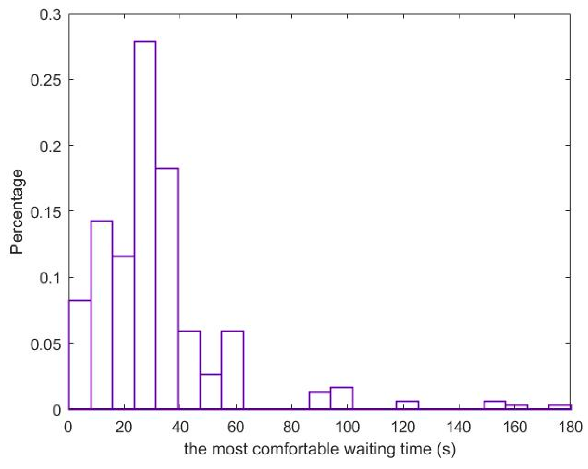
As shown in Figure 2, the collected data of the most comfortable waiting time are relatively concentrated within 1 minute. In this paper, the mean of the collected data is assigned to $T_{comfort}$, i.e., 31 s (0.517 min).

Figure 2. Survey results of the most comfortable waiting time.

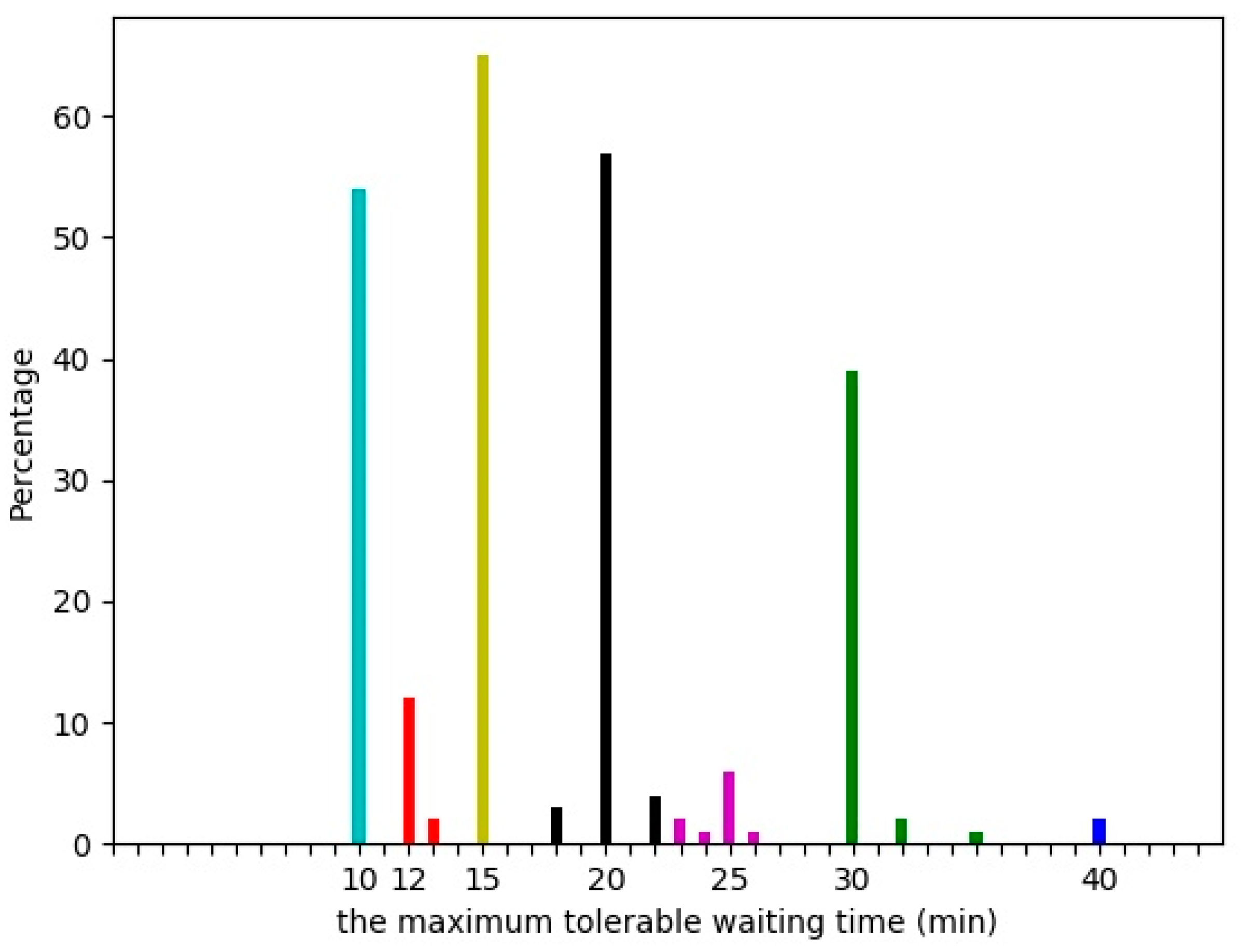
On the other hand, the collected sample data of the maximum tolerable waiting time are more scattered than those of the most comfortable waiting time. Some frequently used distributions, e.g., normal distribution, logistic distribution, log-logistic distribution and lognormal distribution, are used to match these data, but the results are not satisfactory. Thus, we adopt discretization methods in processing the data. K-means cluster analysis is employed to divide survey respondents into seven subsets, and the results are shown in Figure 3 and Table 2.

Figure 3. Sample data distribution in each cluster.

Table 2. Cluster analysis results of sample data on the maximum tolerable waiting time.

Clusters	$\mathbf{Cluster} \mathbf{Centers} ({\mathit{T}}_{\mathit{t}\mathit{o}\mathit{l}\mathit{e}\mathit{r}\mathit{a}\mathit{b}\mathit{l}\mathit{e}}^{}, \mathbf{min})$	Number of Respondents	Percentage
1	10	54	21.51%
2	12	14	5.58%
3	15	65	25.90%
4	20	64	25.50%
5	25	10	3.98%
6	30	42	16.73%
7	40	2	0.80%

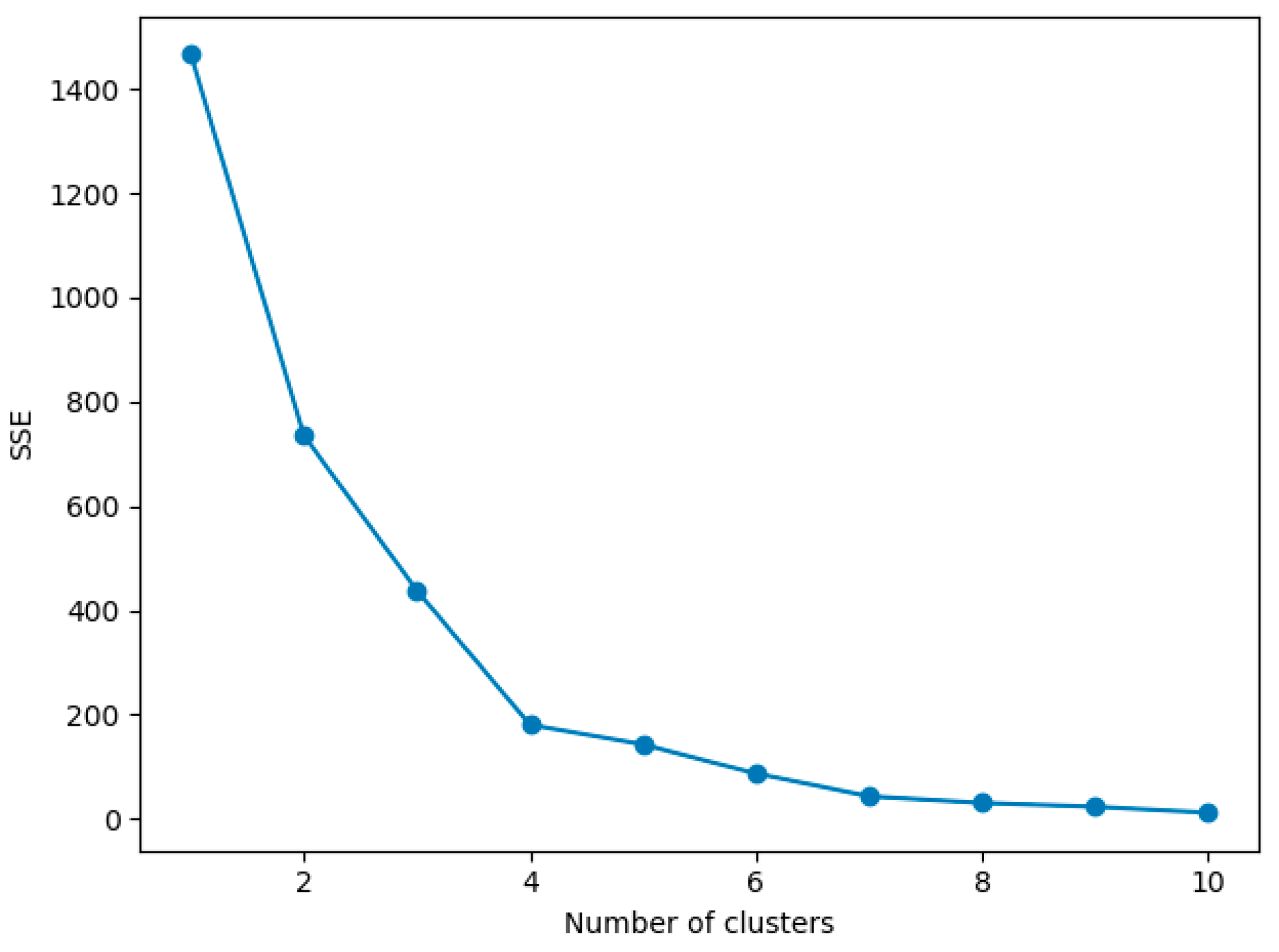
As shown in Figure 4, the sum of the square error (SSE) changes very slightly when the number of clusters is greater than seven. Hence, the number of clusters is set to seven.

Figure 4. SSE for different numbers of clusters.

The results of the cluster analysis are used in the transfer waiting time satisfaction function. Instead of being assigned as a fixed constant, $T_{tolerable}^{}$ differs for each cluster. Passengers are divided into seven groups according to the percentage, and the cluster centers are assigned to each group as $T_{tolerable}^{}$ for passengers in that group.

3. The First Train Timetabling Model

3.1. Assumptions

Assumption 1.

The capacities of trains and facilities in stations can satisfy passengers’ demands. In practice, this is usually the case during the morning periods. Under this assumption, all transfer passengers will board the first available connecting train to reduce their waiting time. Note that travel behaviors and strategies can differ among travelers [39,40], and passengers may give up the first train and choose the following one because of the seat availability [41]. However, in this study passengers are assumed to board the train that arrives first, since the seats are relatively abundant in the early morning.

Assumption 2.

The transfer walking time of passengers for a certain transfer connection in a transfer station is known and fixed. The data can be collected in urban rail transit networks by field experiments or simulations.

Assumption 3.

The passenger transfer demands are relatively stable over a period of time. The demands can be estimated using historical automatic fare collection data.

3.2. Notations

The input parameters and intermediate variables are listed as follows:

• $L$: set of operating lines in the urban rail transit network. $L=\left\{l_i|i=1,2,\cdots ,n\right\}$, where $n$ denotes the total number of lines in the network. $l_i^{+}$ and $l_i^{-}$ represent the up and down directions of $l_i$, respectively.
• $S\left(l_i\right)$: set of operating stations on line $l_i$. $S\left(l_i\right)=\left\{s_j^i|j=1,2,\cdots ,m\right\}$, where m is the total number of stations on line $l_i$.
• $S^{\prime }$: set of the transfer stations in the urban rail transit network. $S^{\prime }=\left\{s_k^{\prime }|k=1,2,\cdots ,w\right\}$, where $w$ is the total number of transfer stations in the network.
• $R_k$: set of the transfer relationships at transfer station $s_k^{\prime }$. $R_k=\left\{r_k^z|z=1,2,\cdots ,q\right\}$, where $q$ is the total number of transfer relationships at $s_k^{\prime }$. Here, a transfer relationship $r_k^z$ means a transfer at station $s_k^{\prime }$ from line direction $l_i^{\ast }$($l_i^{\ast }\in \left\{l_i^{+},l_i^{-}\right\}$) to line direction $l_{i^{\prime }}^{\ast }$($l_{i\prime }^{\ast }\in \left\{l_{i\prime }^{+},l_{i\prime }^{-}\right\}$).
• $C$: set of passenger clusters. $C=\left\{c_x|x=1,2,\cdots ,7\right\}$.
• $T_{s_j\to s_{j+1},l_i^{\ast }}^{run-\min }$: the minimum train running time from station $s_j^i$ to station $s_{j+1}^i$ for line direction $l_i^{\ast }$($l_i^{\ast }\in \left\{l_i^{+},l_i^{-}\right\}$).
• $T_{s_j\to s_{j+1},l_i^{\ast }}^{run-\max }$: the maximum train running time from station $s_j^i$ to station $s_{j+1}^i$ for line direction $l_i^{\ast }$($l_i^{\ast }\in \left\{l_i^{+},l_i^{-}\right\}$).
• $T_{s_j,l_i^{\ast }}^{dwell-\min }$: the minimum train dwell time at station $s_j^i$ for line direction $l_i^{\ast }$($l_i^{\ast }\in \left\{l_i^{+},l_i^{-}\right\}$).
• $T_{s_j,l_i^{\ast }}^{dwell-\max }$: the maximum train dwell time at station $s_j^i$ for line direction $l_i^{\ast }$($l_i^{\ast }\in \left\{l_i^{+},l_i^{-}\right\}$).
• $H_{\min }$: the minimum train headway.
• $H_{\max }$: the maximum train headway.
• $T_{\max }^{origin}$: the maximum changing range of the first train originating time compared to the original timetable.
• $T_{k,z}^{walk}$: the transfer walking time at transfer station $s_k^{\prime }$ for transfer relationship $r_k^{\mathrm{z}}$.
• $D_{k,z}^{transfer}$: the passenger transfer demand at transfer station $s_k^{\prime }$ for transfer relationship $r_k^{\mathrm{z}}$.
• $T_{tolerable}^x$: the maximum tolerable waiting time for passengers in cluster ${\mathrm{c}}_x^{}$.
• $N_{k,z}^{transfer,x}$: the number of transfer passengers in cluster $c_x$ at transfer station $s_k^{\prime }$ for transfer relationship $r_k^{\mathrm{z}}$.
• $T_{\max }^{wait}$: the upper bound of the transfer waiting time among all transfer relationships in the first train timetables.

The decision variables are listed as follows:

• $t_{l_i^{\ast }}^{origin}$: the first train originating time from the depot for line direction $l_i^{\ast }$($l_i^{\ast }\in \left\{l_i^{+},l_i^{-}\right\}$).
• $t_{s_j,l_i^{\ast }}^{depart}$: the first train departure time from station $s_j^i$ for line direction $l_i^{\ast }$($l_i^{\ast }\in \left\{l_i^{+},l_i^{-}\right\}$).
• $t_{s_j,l_i^{\ast }}^{arrival}$: the first train arrival time at station $s_j^i$ for line direction $l_i^{\ast }$($l_i^{\ast }\in \left\{l_i^{+},l_i^{-}\right\}$).
• $t_{s_j\to s_{j+1},l_i^{\ast }}^{run}$: the train running time from station $s_j^i$ to station $s_{j+1}^i$ for line direction $l_i^{\ast }$($l_i^{\ast }\in \left\{l_i^{+},l_i^{-}\right\}$).
• $t_{s_j,l_i^{\ast }}^{dwell}$: the train dwell time at station $s_j^i$ for line direction $l_i^{\ast }$($l_i^{\ast }\in \left\{l_i^{+},l_i^{-}\right\}$).
• $H_{l_i^{\ast }}$: the train headway for line direction $l_i^{\ast }$($l_i^{\ast }\in \left\{l_i^{+},l_i^{-}\right\}$).
• $t_{k,z}^{wait}$: the transfer waiting time at transfer station $s_k^{\prime }$ for transfer relationship $r_k^z$.

3.3. Model Formulations

The optimization objective of the first train timetabling model can be expressed as maximization of the time satisfaction for all first train transfer passengers. For each transfer relationship $r_k^z$ in transfer station $s_k^{\prime }$, the corresponding passenger volume is divided into seven clusters based on the percentage in Table 2. The total time satisfaction can then be calculated by Equation (2).

The model is formulated as follows:

$$\max {\displaystyle \sum _{s_k^{\prime }\in S^{\prime }}{\displaystyle \sum _{r_k^z\in R_k}{\displaystyle \sum _{c_x\in C}F\left(t_{k,z}^{wait},T_{tolerable}^x\right)\times N_{k,z}^{transfer,x}}}}$$

(2)

$$\mathrm{s}.\mathrm{t}. \mathrm{F}(t_{s_k,l_i^{\ast }\to l_{i^{\prime }}^{\ast }}^{wait},T_{tolerable}^x)=\{\begin{array}{l}\frac{1-0.542}{0.517}{t}_{s_k,l_i^{\ast }\to l_{i^{\prime }}^{\ast }}^{wait}+0.542,0\le t_{s_k,l_i^{\ast }\to l_{i^{\prime }}^{\ast }}^{wait}\le 0.517\\ \frac{t_{s_k,l_i^{\ast }\to l_{i^{\prime }}^{\ast }}^{wait}}{0.517-T_{tolerable}^x}-\frac{T_{tolerable}^x}{0.517-T_{tolerable}^x},0.517<t_{s_k,l_i^{\ast }\to l_{i^{\prime }}^{\ast }}^{wait}\le T_{tolerable}^x\\ \frac{{\left(t_{s_k,l_i^{\ast }\to l_{i^{\prime }}^{\ast }}^{wait}\right)}^2-{\left(T_{\max }^{wait}\right)}^2}{{\left(T_{tolerable}^x\right)}^2-{\left(T_{\max }^{wait}\right)}^2}-1,T_{tolerable}^x<t_{s_k,l_i^{\ast }\to l_{i^{\prime }}^{\ast }}^{wait}\le T_{\max }^{wait}\end{array}$$

(3)

$$t_{k,z}^{wait}\in \left[0,T_{\max }^{wait}\right]$$

(4)

$$t_{l_i^{\ast }}^{origin}\in t_{l_i^{\ast }}^{origin}{}^{\prime }\pm T_{\max }^{origin}$$

(5)

$$T_{s_j\to s_{j+1},l_i^{\ast }}^{run-\min }\le t_{s_j\to s_{j+1},l_i^{\ast }}^{run}\le T_{s_j\to s_{j+1},l_i^{\ast }}^{run-\max }$$

(6)

$$T_{s_j,l_i^{\ast }}^{dwell-\min }\le t_{s_j,l_i^{\ast }}^{dwell}\le T_{s_j,l_i^{\ast }}^{dwell-\max }$$

(7)

$$H_{l_i}^{\min }\le H_{l_i^{\ast }}\le H_{l_i}^{\max }$$

(8)

$$t_{s_j\to s_{j+1},l_i^{\ast }}^{run}=t_{s_{j+1},l_i^{\ast }}^{arrival}-t_{s_j,l_i^{\ast }}^{depart}$$

(9)

$$t_{s_j,l_i^{\ast }}^{dwell}=t_{s_j,l_i^{\ast }}^{depart}-t_{s_j,l_i^{\ast }}^{arrival}$$

(10)

$$t_{s_p,l_i^{\ast }}^{arrival}=t_{l_i^{\ast }}^{origin}+{\displaystyle \sum _{j=1}^p{t}_{s_j\to s_{j+1},l_i^{\ast }}^{run}+{\displaystyle \sum _{j=1}^{p-1}{t}_{s_j,l_i^{\ast }}^{dwell}}}$$

(11)

$$t_{k,z}^{wait}=t_{s_k,l_{i^{\prime }}^{\ast }}^{depart}+\alpha \times H_{l_{i^{\prime }}^{\ast }}-\left(t_{s_k,l_i^{\ast }}^{arrival}+T_{k,z}^{walk}\right)\left(\alpha \in N\right)$$

(12)

Constraint (4) restricts the domain of the decision variables $t_{k,z}^{wait}$. Constraint (5) limits the optimized originating time of the first trains in the time scope around the original timetables, where $t_{l_i^{\ast }}^{origin}{}^{\prime }$ denotes the first train originating time for line direction $l_i^{\ast }$ in the original timetable. The originating times cannot be brought forward to an extent that increases the operational costs, or postponed to the extent that passengers’ originating waiting time increases. Constraint (6) is the train running limit, that is determined by the pure running time on a segment and the durations of train start-up and pull-up. Constraint (7) is the train dwelling limit in a station, which is influenced mainly by the volume of boarding and alighting passengers. Constraint (8) is a basic condition to guarantee that two consecutive trains maintain a safe running interval. The transfer waiting time in the objective function can be calculated with Constraints (9)–(12). If the first train of connecting line direction $l_{i^{\prime }}^{\ast }$ departs later than the arrival of transfer passengers of the first train of the feeder line direction $l_i^{\ast }$ at the platform of $l_{i^{\prime }}^{\ast }$, parameter $\alpha$ in Constraint (12) will be zero; otherwise,$\alpha$ will be greater than zero.

4. Solution Algorithm

4.1. Artificial Bee Colony Algorithm

Due to the large number of decision variables, the first train timetabling model has an extremely large solution space. The artificial bee colony (ABC) algorithm is an optimization technique that simulates the foraging behavior of honey bees and has been successfully applied to various practical problems [42]. We utilize the ABC algorithm in solving the proposed optimization model.

In the ABC algorithm, the colony consists of three groups of bees: employed bees, onlookers and scouts. The goal of the whole colony is to find the largest nectar source. Employed bees go to their food source and return to the hive and dance on this area. An employed bee whose food source has been abandoned becomes a scout and starts to search for a new food source. Onlookers watch the dances of employed bees and choose food sources depending on the dances [42]. The detailed steps of the algorithm are given below:

Step 1: initialization

(1) Input the model parameters: $L$, $S\left(l_i\right)$, $S^{\prime }$, $R_k$, $C$, $T_{s_j\to s_{j+1},l_i^{\ast }}^{run-\min }$, $T_{s_j\to s_{j+1},l_i^{\ast }}^{run-\max }$, $T_{s_j,l_i^{\ast }}^{dwell-\min }$, $T_{s_j,l_i^{\ast }}^{dwell-\max }$, $H_{\min }$, $H_{\max }$, $T_{\max }^{origin}$, $T_{k,z}^{walk}$, $D_{k,z}^{transfer}$, $T_{tolerable}^x$ and $T_{\max }^{wait}$;

(2) Set the initial ABC parameters: number of food sources $N_{food}$, maximum number of iterations $N_{iteration}^{\max }$, maximum number of no-updates of a food source $N_{noupdate}^{\max }$, and maximum number of no-updates of the largest nectar source $N_{best}^{\max }$;

(3) Initialize food sources $x_i$($i=1,2,\cdots ,N_{food}$). Each food source consists of the first train originating time, train running time, train dwell time and train headway of each line direction in the urban rail transit network (see Figure 5).

Figure 5. Composition of a Food Source.

(4) Calculate the nectar amount $Z_i$($i=1,2,\cdots ,N_{food}$) (corresponding to the objective function value, i.e., the total time satisfaction) for initial food sources, and find and record the largest nectar source $x_{best}$.

(5) Set the initial number of iterations $N_{iteration}$ to be 1. Set the number of no-updates of $x_i$($i=1,2,\cdots ,N_{food}$) $N_{noupdate,i}$ to be 0. The number of no-updates of the largest nectar source $N_{best}$ is set to 0.

Step 2: employed bees stage

Update the current food sources. For each food source $x_i$, select another food source $x_k$($k\ne i$) randomly and generate a new food source $x_i{}^{\prime }$ via Equation (13). Compare the nectar amounts of $x_i$ and $x_i{}^{\prime }$. If the former is larger than the latter, update $x_i$ to $x_i{}^{\prime }$; otherwise, keep $x_i$ unchanged and $N_{noupdate,i}=N_{noupdate,i}+1$.

$$x_{i,j}^{\prime }=\{\begin{array}{l}{x}_{i,j}-{\phi }_{i,j}(x_{i,j}-x_{k,\mathrm{j}}),x_{i,j}>x_{k,j}\\ x_{i,j}+{\phi }_{i,j}(x_{k,j}-x_{i,j}),x_{i,j}<x_{k,j}\end{array}$$

(13)

where $x_{i,j}$ is the value of the j-th variable in $x_i$ and ${\phi }_{i,j}$ is a random number between 0 and 1.

Step 3: onlooker bees stage

(1) Calculate the nectar amount for new food sources generated in Step 2. The selection probability of each food source is determined by Equations (14)–(16).

$$M=\frac{1}{N_{food}}\times {\displaystyle \sum _{i=1}^{N_{food}}{Z}_i}$$

(14)

$$F_i=e^{-(\frac{M}{Z_i})},i=1,2,\dots ,n$$

(15)

$$P_k=\frac{F_k}{{\displaystyle {\sum }_{i=1}^n{F}_i}},i=1,2,\dots ,n$$

(16)

where $Z_i$ is the nectar amount of food source $x_i$ and $P_k$ is the selection probability of food source $x_k$.

(2) Use roulette selection to update the current food sources. The updating methods are similar to those in the employed bee stage.

Step 4: scout bees stage

Update the food sources for which the number of no-updates is larger than $N_{noupdate}^{\max }$ via Equation (17).

$$x_{i,j}^{\prime }=x_{i.j}^{\min }+{\delta }_{i,j}\left(x_{i.j}^{\max }-x_{i.j}^{\min }\right)$$

(17)

where $x_{i.j}^{\min }$ and $x_{i.j}^{\max }$ are the minimum value and maximum value of the j-th variable in $x_i$, respectively, and ${\delta }_{i,j}$ is a random number between 0 and 1.

Step 5: stop or not

(1) Calculate the nectar amount $Z_i$($i=1,2,\cdots ,N_{food}$) for the current food sources and find the current largest nectar source $x_{best}^{\prime }$.

(2) Compare $x_{best}^{\prime }$ and $x_{best}$. If $x_{best}^{\prime }=x_{best}$, $N_{best}=N_{best}+1$. If $N_{best}\ge N_{best}^{\max }$, stop.

(3) Set $N_{iteration}=N_{iteration}+1$. If $N_{iteration}\ge N_{iteration}^{\max }$, stop; otherwise, return to Step 2.

4.2. A Sample Test

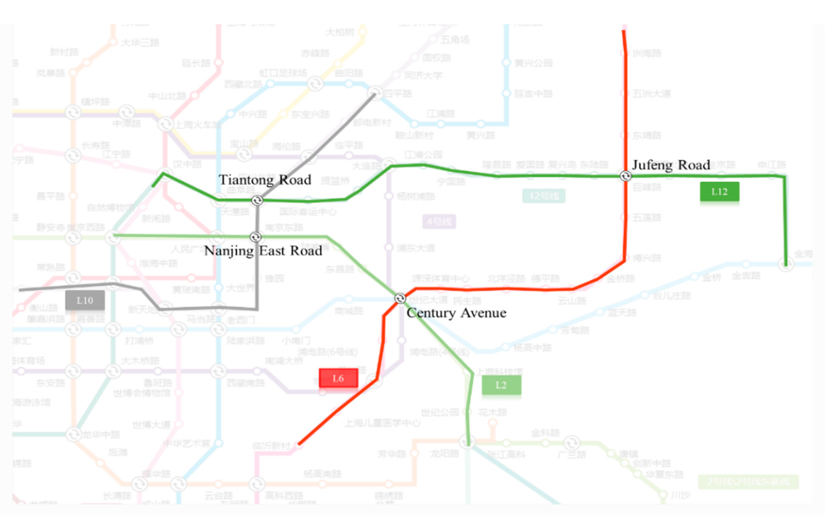
A sample network with four bidirectional operating lines is shown in Figure 6. This network, which is part of the Shanghai urban rail transit network, has 4 transfer stations and 61 non-transfer stations.

Figure 6. A sample network.

The assigned values of some parameters in the model and ABC algorithm are shown in Table 3.

Table 3. Assigned values of some parameters.

Parameters	${\mathit{H}}_{\mathbf{min}}$	${\mathit{H}}_{\mathbf{max}}$	${\mathit{T}}_{\mathbf{max}}^{\mathit{o}\mathit{r}\mathit{i}\mathit{g}\mathit{i}\mathit{n}}$	${\mathit{T}}_{\mathbf{max}}^{\mathit{w}\mathit{a}\mathit{i}\mathit{t}}$	${\mathit{N}}_{\mathit{f}\mathit{o}\mathit{o}\mathit{d}}$	${\mathit{N}}_{\mathit{i}\mathit{t}\mathit{e}\mathit{r}\mathit{a}\mathit{t}\mathit{i}\mathit{o}\mathit{n}}^{\mathbf{max}}$	${\mathit{N}}_{\mathit{n}\mathit{o}\mathit{u}\mathit{p}\mathit{d}\mathit{a}\mathit{t}\mathit{e}}^{\mathbf{max}}$	${\mathit{N}}_{\mathit{b}\mathit{e}\mathit{s}\mathit{t}}^{\mathbf{max}}$
Assigned value	7 min	11 min	±15 min	80 min	50	1000	100	100

The optimization results for the sample network are displayed in Table 4 and Table 5 and Figure 7. As shown in Table 4, compared to the original timetables, the first train originating times of six line directions are brought forward, and the other two are postponed. By means of these adjustments, the total waiting time satisfaction of all the first train transfer passengers is increased by 44.31%, and 71.88% of all the transfer relationships are improved in terms of time satisfaction (see Table A2 in Appendix B).

Table 4. Comparison on the first train originating times and headways.

$\mathbf{Line} \mathbf{Direction} {\mathit{l}}_{\mathit{i}}^{\ast }$	$\mathbf{Original} \mathbf{First} \mathbf{Train} \mathbf{Originating} \mathbf{Time} {\mathit{t}}_{{\mathit{l}}_{\mathit{i}}^{\ast }}^{\mathit{o}\mathit{r}\mathit{i}\mathit{g}\mathit{i}\mathit{n}}{}^{\prime }$	$\mathbf{Optimized} \mathbf{First} \mathbf{Train} \mathbf{Originating} \mathbf{Time} {\mathit{t}}_{{\mathit{l}}_{\mathit{i}}^{\ast }}^{\mathit{o}\mathit{r}\mathit{i}\mathit{g}\mathit{i}\mathit{n}}$	Original Headway	Optimized Headway
$l_2^{+}$	5:28:00	5:21:00	8	8
$l_2^{-}$	5:10:00	5:23:00	8	9
$l_6^{+}$	5:30:00	5:22:00	8	8
$l_6^{-}$	5:30:00	5:24:00	8	9
$l_{10}^{+}$	5:30:00	5:15:00	8	8
$l_{10}^{-}$	5:25:00	5:30:00	8	8
$l_{12}^{+}$	5:30:00	5:24:00	9	9
$l_{12}^{-}$	5:30:00	5:24:00	9	7

Table 5. Comparison of the original timetable and the optimized timetable

	Original	Optimized	Change	Percentage
The total time satisfaction	1354	1954	600	+44.31%
The number of transfer passengers within the maximum tolerable waiting time	1921	2170	249	+12.96%
The total transfer waiting time (min·person)	17065	5242	−11,823	−69.28%
The average transfer waiting time (min/person)	7.75	2.38	−5.37	−69.29%

Figure 7. Comparison of the number of transfer passengers in different time frames.

As displayed in Table 5, in terms of the pure transfer time, the total transfer time is reduced by 69.28%, and the average transfer time is decreased from 7.75 min to 2.38 min. Meanwhile, the number of transfer passengers within the maximum tolerable waiting time rises by 249. As seen in Figure 7, the number of transfer passengers with transfer waiting times below 5 min increases substantially, and the number of transfer passengers with waiting times exceeding 5 min decreases considerably. In particular, the number of passengers whose transfer waiting time is less than the most comfortable waiting time (31 s) is reduced to zero, which implies that the optimized timetable can better protect train connections against small delays. On the other hand, the transfer waiting times for over 90% of all transfer passengers are less than 20 min after optimization, so the timetable is improved with respect to extremely long waiting times.

5. Case Study

5.1. Optimization Results

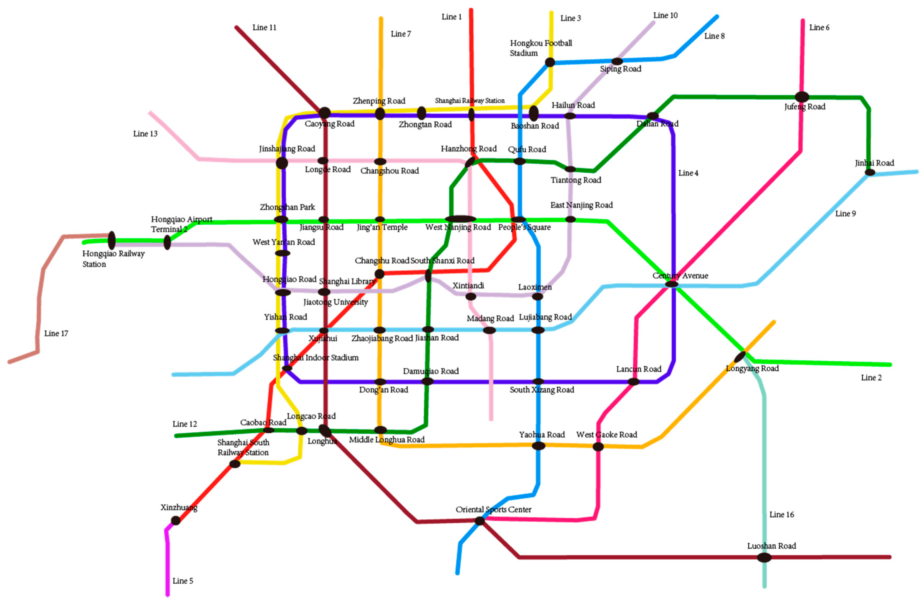
To verify the performance of our model and algorithm, we conducted a case study on the real-life urban rail transit network in Shanghai. As shown in Figure 8, the Shanghai network consists of 15 bidirectional lines and 43 transfer stations.

Figure 8. Map of the Shanghai urban rail network.

The parameters in the model and ABC algorithm are assigned the same values as in the test sample, as shown in Table 3. Data on the passenger volume of the first train transfer passengers are provided by the Beijing rail transit company.

Compared to the original timetables, the first train originating times in the optimized timetables are either brought forward or postponed within 10 min (see Table A3 in Appendix B). Moreover, the optimized headways are closer to each other than the original headways (see Table A3 in Appendix B). As shown in Table 6, these adjustments result in an increase of 32.77% in the total time satisfaction of all the first train transfer passengers. Meanwhile, 3010 more transfer passengers have a transfer waiting time shorter than the maximum tolerable waiting time. With respect to the pure transfer time, the total transfer time is decreased by 35.55%, and the average transfer time is decreased from 9.43 min to 6.07 min.

Table 6. Comparison of the original timetable and the optimized timetable.

	Original	Optimized	Change	Percentage
The total time satisfaction	18,555	24,636	6081	+32.77%
The number of transfer passengers within the maximum tolerable waiting time	28,341	31,351	3010	+10.62%
The total transfer waiting time (min· person)	324,831	209,340	−115,491	−35.55%
The average transfer waiting time (min/person)	9.43	6.07	−3.36	−35.63%

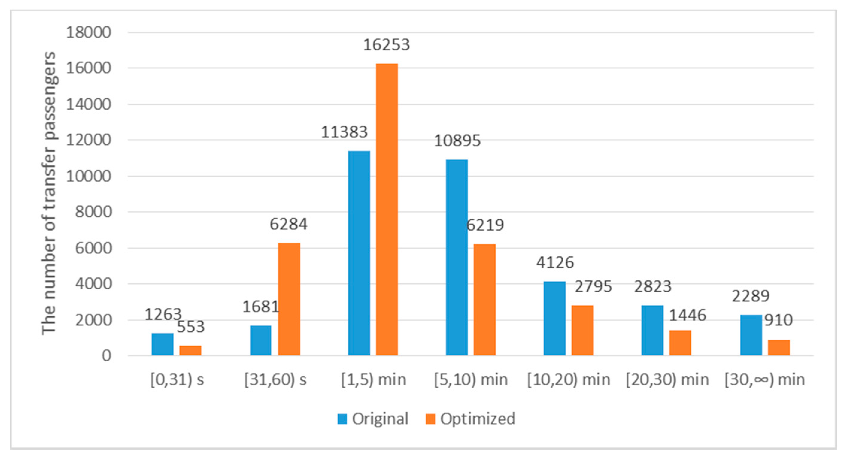
As shown in Figure 9, the number of transfer passengers with a transfer time less than 31 s or greater than 5 min decreases significantly, while the number of passengers with a transfer time around [31 s, 5 min) shows an obvious increase (from 13,064 persons to 23,090 persons, improving by 76.75%). This reveals that through optimization, more passengers would experience a relatively comfortable waiting time. On one hand, fewer passengers suffer from the stress and tension caused by excessively short transfer waiting times. On the other hand, the optimization also achieves good performance with respect to reducing the extremely long waits.

Figure 9. Comparison of the number of transfer passengers in different time frames.

5.2. Analysis of the Results of Publishing Timetables

Although occurrences of the extremely long wait phenomenon have been reduced after using the optimized timetables, the phenomenon still arises for passengers transferring from the first train of one line direction to the first train of another line direction. The connecting train arrives at the transfer station much later than the feeder train, so transfer passengers have to wait for a long time. If we make the timetables public to passengers via mass media, passengers may choose to take a later train instead of the first train of the feeder line direction to reduce their transfer waiting time. Based on this idea, we conduct an experiment to test the effects of publishing timetables.

In the experiment, transfer passengers choose the train with the highest transfer time satisfaction calculated according to Equation (3), and the results are shown in Table 7. Table 8 demonstrates the changes in transfer waiting time for some transfer stations. After publishing the timetables, extremely long waits are completely eliminated, the average transfer waiting time is cut in half, and the total time satisfaction is increased by 16.38%. These results provide good insight for urban rail transit agencies in providing train timetable information to the public.

Table 7. Comparison of the optimization results before and after timetable publication.

	Before	After	Change	Percentage
The total time satisfaction	24,636	286,72	4036	+16.38%
The number of transfer passengers within the maximum tolerable waiting time	31,351	34,457	3106	+9.91%
The total transfer waiting time (min· person)	209,340	101,767	−107,573	−51.39%
The average transfer waiting time (min/ person)	6.07	2.95	−3.12	−51.40%

Table 8. Comparison of the transfer waiting time at some stations before and after timetable publication.

$\mathbf{Transfer} \mathbf{Station} {\mathit{S}}^{\prime }$	$\mathbf{Transfer} \mathbf{Relationship} {\mathit{R}}_{\mathit{k}}$	Transfer Waiting Time
		Before Publication	After Publication
Jiangsu Road	Line2Down→line11Up	59′15″	3′15″
	Line2Up→line11Up	52′18″	7′18″
Longde Road	Line13Up→line11Up	55′38″	6′38″
	Line13Down→line11Up	37′19″	5′19″
Caoyang Road	Line3Down→line11Up	33′2″	6′2″
West gaoke Road	Line6Up→line7Up	35′24″	0′24″
Jiashang Road	Line12Down→line9Up	32′52″	4′52″
Century Avenue	Line6Up→line9Up	39′54″	7′54″
Longhua Road	Line12Up→line11Up	41′9″	6′9″

5.3. Comparison with the Results of Minimizing the Transfer Waiting Time

As mentioned in the introduction, researchers generally optimize the first train timetable by minimizing the total transfer waiting time. In this chapter, we compare the results between optimization with two different goals, i.e., minimizing the total transfer waiting time and maximizing the total waiting time satisfaction. The results are shown in Table 9 and Figure 10.

Table 9. Comparison of the optimization results with two different goals.

	Minimize Transfer Waiting Time	Maximize Waiting Time Satisfaction	Difference	Percentage
The total time satisfaction	22,748	24,636	1888	+8.30%
The number of transfer passengers within the maximum tolerable waiting time	31,418	31,351	−67	−0.21%
The total transfer waiting time (min· person)	201,863	209,340	7477	+3.70%
The average transfer waiting time (min/person)	5.86	6.07	0.21	+3.58%

Figure 10. Comparison of the number of transfer passengers in different time frames.

Compared to the minimization goal, although the maximization goal leads to a slight increase in transfer waiting time, it produces an 8.30% improvement in time satisfaction. More importantly, the maximization goal has better performance in terms of decreasing the number of extremely short waits (from 6942 to 553), which make passengers nervous. Therefore, “just miss” events can be avoided with the maximization optimization goal. Meanwhile, the number of passengers with a relatively comfortable waiting time around [31 s, 5 min) increases by 48.13%.

5.4. Convergence Test

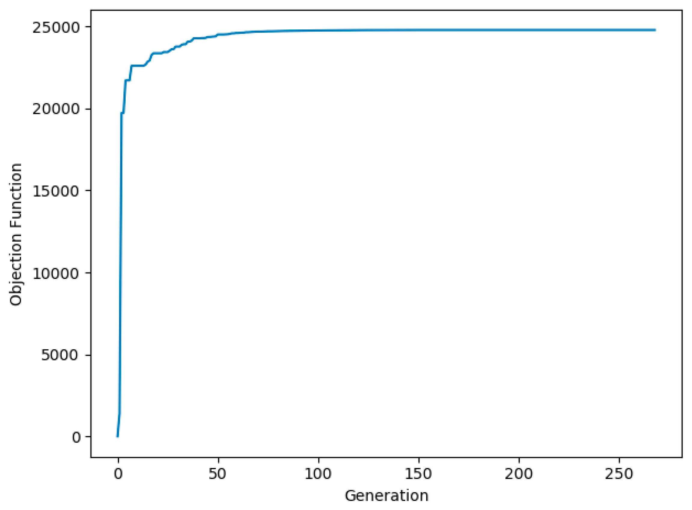
A convergence test of the objective function is conducted for the ABC algorithm. As demonstrated in Table 10, 266 iterations were performed in 8 min and 41 s to reach the best solution of 24,636 for the objective function. In addition, we compare the performance of the ABC algorithm and the Genetic algorithm (see Figure 11 and Figure 12), using Python on a computer with a 4 × 2.5 GHz CPU and 8 GB RAM. Obviously, the ABC algorithm performs better in terms of convergence speed and solution quality.

Table 10. Comparison of the ABC algorithm and Genetic algorithm (GA).

Algorithm	Objective Function Value	Number of Iterations	CPU Time
ABC algorithm	24,636	266	8′41″
GA	22,960	249	22′46″

Figure 11. Convergence of the ABC algorithm

Figure 12. Convergence of GA.

6. Conclusions

This paper solved the challenging problem of first train timetabling considering transfer coordination, which is significant in improving the quality of transfer service for urban rail transit networks. A first train timetabling model was proposed with the goal of maximizing passenger transfer waiting time satisfaction. To construct the relationship between transfer waiting time and passenger satisfaction, a reference-based time satisfaction function was formulated, with the consideration of passengers’ dissatisfaction on “just miss” and passengers’ balking behavior. An artificial bee colony algorithm was applied to solve the timetabling model. Finally, the results of a case study verify the effectiveness and efficiency of the proposed model and algorithm.

The following specific suggestions are proposed based on the results: (1) To avoid “just miss” scenarios, it is more favorable to set apart some time for transfer waiting than to create zero waiting. The most comfortable waiting time for transfer passengers is 31 s. (2) The headways of rail lines can be set closer to each other, resulting in better train connections between different lines. (3) Urban rail transit agencies can make the train timetables public to passengers via mass media, so as to reduce passenger transfer waiting time. (4) Instead of minimizing the total transfer waiting time, optimizing the first train timetables with the goal of maximizing the total transfer waiting time satisfaction yields better results, in eliminating “just miss” events and increasing the number of passengers encountering comfortable transfer waiting times.

There are still some limitations to our study. First, in our study, a SP survey conducted in Shanghai helped to acquire passengers’ response on the three undetermined parameters $T_{comfort}$, $T_{tolerable}^{}$ and $T{S}_{zero-waiting}$ in the waiting time satisfaction function. The reason we chose Shanghai was that, as discussed, the passengers with abundant transfer experiences during their daily commuting in the Shanghai rail transit network fit the experience-based nature of the survey. Further, our case study was conducted on the Shanghai rail transit network, so determining the parameters based on the field survey in Shanghai made the optimization results of the case study more credible. However, due to fund limitation and the cooperation issue of respondents, the sample size was not so big. Furthermore, our collected data only involved passengers in Shanghai, but passengers’ responses may vary due to their different regions. A larger survey on the spot or on the internet can be done in future research, to further expand sample size and improve the sample representativeness, so that we can better examining passengers’ reactions on the three parameters. Second, the waiting time satisfaction function was formulated as a linear function in our study. Further work may explore whether nonlinear functions can be utilized, and which form performs better.

References

1. Szpigel, B. Optimal train scheduling on a single track railway. Oper. Res. 1973, 34, 343–352. [Google Scholar]
2. Lee, K.K.T.; Schonfeld, P. Optimal slack time for timed transfers at a transit terminal. J. Adv. Transp. 1991, 25, 281–308. [Google Scholar] [CrossRef]
3. Chien, F.; Schonfeld, P. Joint optimization of a rail transit line and its feeder bus system. J. Adv. Transp. 1998, 32, 253–284. [Google Scholar] [CrossRef]
4. Chowdhury, S.M.; Chien, S.I. Intermodal transit system coordination. Transp. Plan. Technol. 2002, 25, 257–287. [Google Scholar] [CrossRef]
5. Vansteenwegen, P.; Oudheusden, D.V. Decreasing the passenger waiting time for an intercity rail network. Transp. Res. Part B 2007, 41, 478–492. [Google Scholar] [CrossRef]
6. Li, S.J.; Xu, R.H.; Han, K. Demand-oriented train services optimization for a congested urban rail line: Integrating short turning and heterogeneous headways. Transp. A Transp. Sci. 2019, 15, 1459–1486. [Google Scholar] [CrossRef]
7. Xue, Q.C.; Yang, X.; Wu, J.J.; Sun, H.J.; Yin, H.D.; Qu, Y.C. Urban rail timetable optimization to improve operational efficiency with flexible routing plans: A nonlinear integer programming model. Sustainability 2019, 11, 3701. [Google Scholar] [CrossRef] [Green Version]
8. Wang, Y.H.; Tang, T.; Ning, B.; Boom, T.J.J.; Schutter, B.D. Passenger-demands-oriented train scheduling for an urban rail transit network. Transp. Res. Part C 2015, 60, 1–23. [Google Scholar] [CrossRef]
9. Zhou, W.L.; Fan, W.Z.; You, X.R.; Deng, L.B. Demand-oriented train timetabling integrated with passenger train-booking decisions. Sustainability 2019, 11, 4932. [Google Scholar] [CrossRef] [Green Version]
10. Yang, X.; Li, X.; Gao, Z.; Wang, H.; Tang, T. A cooperative scheduling model for timetable optimization in subway systems. IEEE Trans. Intell. Transp. Syst. 2013, 14, 438–447. [Google Scholar] [CrossRef]
11. Chakroborty, P.; Deb, K.; Subrahmanyam, P.S. Optimal scheduling of urban transit systems using genetic algorithms. J. Transp. Eng. 1995, 121, 544–553. [Google Scholar] [CrossRef]
12. Goverde, R.M.P. Optimal Scheduling of Connections in Railway Systems; Technical Report No. 929; Delft University of Technology: Delft, The Netherlands, 1998. [Google Scholar]
13. Kwan, C.M.; Chang, C.S. Timetable synchronization of mass rapid transit system using multiobjective evolutionary approach. IEEE Trans. Syst. 2008, 38, 636–648. [Google Scholar] [CrossRef]
14. Zhou, W.L.; Deng, L.B.; Xie, M.Q.; Yang, X. Coordination optimization of the first and last trains’ departure time on urban rail transit network. Adv. Mech. Eng. 2013, 5, 848292. [Google Scholar] [CrossRef]
15. Wu, J.J.; Liu, M.H.; Sun, H.J.; Li, T.F.; Gao, Z.Y.; Wang, D.Z.W. Equity-based timetable synchronization optimization in urban subway network. Transp. Res. Part C 2015, 51, 1–18. [Google Scholar] [CrossRef]
16. Shi, R.J.; Mao, B.H.; Ding, Y.; Bai, Y.; Chen, Y. Timetable optimization of rail transit loop line with transfer coordination. Discret. Dyn. Nat. Soc. 2016, 2016, 4627094. [Google Scholar] [CrossRef] [Green Version]
17. Shang, P.; Li, R.; Liu, Z.; Xian, K.; Guo, J. Timetable synchronization and optimization considering time-dependent passenger demand in an urban subway network. Transp. Res. Rec. 2018, 2672, 243–254. [Google Scholar] [CrossRef]
18. Chen, Y.; Mao, B.H.; Bai, Y.; Ho, T.K.; Li, Z.J. Timetable synchronization of last trains for urban rail networks with maximum accessibility. Transp. Res. Part C 2019, 99, 110–129. [Google Scholar] [CrossRef]
19. Zhou, Y.; Wang, Y.; Yang, H.; Yan, X.D. Last train scheduling for maximizing passenger destination reachability in urban rail transit networks. Transp. Res. Part B 2019, 129, 79–95. [Google Scholar] [CrossRef]
20. Kang, L.J.; Zhu, X.N. A simulated annealing algorithm for first train transfer problem in urban railway networks. Appl. Math. Model. J. 2016, 40, 419–435. [Google Scholar] [CrossRef]
21. Kang, L.J.; Zhu, X.N.; Sun, H.J.; Puchinger, J.; Ruthmair, M.; Hu, B. Modeling the first train timetabling problem with minimal missed trains and synchronization time differences in subway networks. Transp. Res. Part B 2016, 93, 17–36. [Google Scholar] [CrossRef] [Green Version]
22. Guo, X.; Wu, J.J.; Sun, H.J.; Liu, R.H.; Gao, Z.Y. Timetable coordination of first trains in urban railway network: A case study of Beijing. Appl. Math. Model. 2016, 40, 8048–8066. [Google Scholar] [CrossRef] [Green Version]
23. Ning, L.Q.; Zhao, P.; Xu, W.K.; Qiao, K. Transfer Coordination for Metro Networks during the Start- or End-of-Service Period. Math. Probl. Eng. 2018, 2018, 3835270. [Google Scholar] [CrossRef]
24. Schroder, M.; Solchenbach, I. Optimization of Transfer Quality in Regional Public Transit; Technical Report No. 84; Berichte des Fraunhofer Instituts for Techno-und Wirtschafts: Munich, Germany, 2006. [Google Scholar]
25. Wang, Y.B.; Guo, J.Q.; Ceder, A.; Currie, G.; Dong, W.; Yuan, H. Waiting for public transport services: Queueing analysis with balking and reneging behaviors of impatient passengers. Transp. Res. Part B 2014, 63, 53–76. [Google Scholar] [CrossRef]
26. Barrer, D.Y. Queuing with impatient customers and indifferent clerks. Oper. Res. 1957, 5, 644–649. [Google Scholar] [CrossRef]
27. Maister, D. The Psychology of Waiting Lines. In The Service Encounter; Lexington Books: Lexington, KY, USA, 1985; pp. 13–23. [Google Scholar]
28. Davis, M.M.; Maggard, M.J. An analysis of customer satisfaction with waiting times in a two-stage service. J. Oper. Manag. 1990, 9, 324–334. [Google Scholar] [CrossRef]
29. Carmon, Z.; Shanthikumar, J.G.; Freed, T. A psychological perspective on service segmentation models: The significance of accounting for consumers’ perceptions of waiting and service. Manag. Sci. 1995, 41, 1806–1815. [Google Scholar] [CrossRef] [Green Version]
30. Durrande-Moreau, A. Waiting for service: Ten years of empirical research. Int. J. Serv. Ind. Manag. 1999, 10, 171–194. [Google Scholar] [CrossRef]
31. Wong, R.C.W.; Yuen, T.W.Y.; Fung, K.W.; Leung, J.M.Y. Optimizing timetable synchronization for rail mass transit. Transp. Sci. 2008, 42, 57–69. [Google Scholar] [CrossRef]
32. Miller, J.A. Studying satisfaction, modifying models, eliciting expectations, posing problems, and making meaningful measurements. In Conceptualization and Measurement of Consumer Satisfaction and Dissatisfaction; Hunt, H.K., Ed.; Marketing Science Institute (May): Cambridge, MA, USA, 1977; pp. 72–91. [Google Scholar]
33. Churchill, G.A.; Surprenant, C. An investigation into the determinants of customer satisfaction. J. Mark. Res. 1982, 19, 491–504. [Google Scholar] [CrossRef]
34. Palawatta, T.M.B. Waiting Times and Defining Customer Satisfaction. Vidyojaya J. Manag. 2015, 1, 15–24. [Google Scholar] [CrossRef]
35. Shang, H.Y.; Huang, H.J.; Wu, W.X. Bus timetabling considering passenger satisfaction: An empirical study in Beijing. Comput. Ind. Eng. 2019, 135, 1155–1166. [Google Scholar] [CrossRef]
36. Gao, Y.N.; Rasouli, S.; Timmermans, H.; Wang, Y.Q. Trip stage satisfaction of public transport users: A reference-based model incorporating trip attributes, perceived service quality, psychological disposition and difference tolerance. Transp. Res. Part A 2018, 118, 759–775. [Google Scholar] [CrossRef]
37. Cats, O. Dynamic Modelling of Transit Operations and Passenger Decisions. Ph.D. Thesis, KTH, School of Architecture and the Built Environment (ABE), Transport Science, Traffic and Logistics, Stockholm, Sweden, 2011. [Google Scholar]
38. Abenoza, R.F.; Cats, O.; Susilo, Y.O. Travel satisfaction with public transport: Determinants, user classes, regional disparities and their evolution. Transp. Res. Part A 2017, 95, 64–84. [Google Scholar] [CrossRef] [Green Version]
39. Nuzzolo, A.; Comi, A. A Subjective Optimal Strategy for Transit Simulation Models. J. Adv. Transp. 2018, 2018, 8797328. [Google Scholar] [CrossRef]
40. Wang, J.; Peeta, S.; He, S. Multiclass traffic assignment model for mixed traffic flow of human-driven vehicles and connected and autonomous vehicles. Transp. Res. Part B Methodol. 2019, 126, 139–168. [Google Scholar] [CrossRef]
41. Schmöcker, J.D.; Fonzone, A.; Shimamoto, H.; Kurauchi, F. Frequency-based transit assignment considering seat capacities. Transp. Res. Part A 2011, 45, 392–408. [Google Scholar] [CrossRef]
42. Karaboga, D. An Idea Based on Honey Bee Swarm for Numerical Optimization; Technical Report-TR06; Erciyes University: Kayseri, Turkey, 2005. [Google Scholar]