Abstract
Mid- and long-term monitoring of restoration projects have to be performed, as short-term evaluations do not give comprehensive information about their outcomes. In this study, we assessed the results of a forest restoration project, implemented in former road builder’s yards. We evaluated the recovery of the soil’s physical and chemical properties, the effectiveness and naturalness of sward restoration, and the success of woody species planting. Our hypotheses were that soil–plant interaction strongly influenced the restoration dynamics. The areas were restored in 2016. In 2014, we collected data from 28 restored areas. Eight years after the restoration, the physical and chemical properties of the soil indicated good quality. Suitable soil conditions were reflected in the herbaceous vegetation cover, which was higher than 60% in all the areas. The sown mixture successfully contained spontaneous species, and perennials prevailed over annuals, indicating stability in the composition of the sward. Alien species cover (generally < 10%) was controlled by sown species. Sown species also outcompeted ruderal and typical grassland species, reducing the naturalness of the herbaceous layer. Tree and shrub growth was low, and soil properties did not affect their height. Our results underline the importance of sowing an herbaceous species mixture in degraded areas in order to efficiently restore the soil cover and to reduce the colonization of alien species. Moreover, in our study, we showed how soil properties differently affected plant species groups.
1. Introduction
The aim of restoration ecology is to counteract human impact on the environment, through the creation of an ecosystem that is self-supporting and resilient to future disturbances [1]. To accomplish this aim, throughout restoration planning it is necessary to identify both the abiotic factors (e.g., water table, microclimatic conditions, physical and chemical properties of the soil) that have to be restored and the herbaceous, shrub, and tree species suitable for the restoration of the ecosystem [2,3,4,5].
Monitoring over time has to be planned prior to the implementation of the restoration as well, in order to evaluate the success of restoration techniques, to adjust restoration actions, and to adapt management strategies [6]. Nevertheless, several restoration projects lack medium- and long-term follow-up management. Monitoring is usually carried out for a period of 3 to 5 years [7], but according to [8], essential components of the ecosystem develop over approximately 25 years; thus, monitoring should also continue after the initial stages of the restoration.
The identification of criteria that characterize an effective, efficient, and successful project is the first step to improving any monitoring actions [1]. Most studies try to assess forest restoration success by measuring species diversity, vegetation structure, and ecological processes (e.g., nutrient cycling, soil organic matter, mycorrhizae) [9,10]. Measures of these parameters provide useful information about the dynamics occurring in the ecosystem. They help in predicting future pathways and give information about processes and cycles necessary for habitat stability over time [11].
However, the building of infrastructure, such as railways and highways, strongly affects the regeneration niche. Building activities entail vegetation removal and soil manipulation (i.e., soil stripping, stocking, and re-spreading) [12], which reduce soil quality. The soil is essential for plant establishment, development, and survival, as it fosters nutrients, regulates the water cycle, and provides anchorage for roots [13]. Soil can be recovered through mechanical site preparation and fertilizer addition, which improve physical and chemical properties of soil [14,15]. These properties may affect plant establishment and composition, and plant–soil interaction may change over time. Thus, restoration projects and monitoring have to focus not only on vegetation but also on soil recovery in builder’s yards because soil health and fertility are key factors affecting sward and forest restoration [16,17].
To our knowledge, few works assessed the relative importance of physical and chemical properties of soil in conditioning the vegetation colonization process in restored areas. In our study, we investigated restoration outcomes eight years after its implementation, in the context of a large lowland deciduous forest restoration project. We investigated sward restoration and woody species growth in a restored area interested by railway construction works, focusing on soil properties’ effect on the development of different vegetation groups. We hypothesized that soil properties and plant–plant interaction may have considerably influenced the restoration. Our main aims were thus to (1) evaluate the soil’s physical and chemical parameters, (2) assess the effectiveness of sward restoration, (3) evaluate the naturalness of sward restoration, and (4) assess the effectiveness of the plantation.
2. Materials and Methods
2.1. Study Site
The survey was carried out at 28 restored sites in the Po Plain, Northwestern Italy. The areas were located along an 84.6 km segment of Rail Freight Corridor 6, the “Mediterranean Corridor” [18], linking the Southwestern Mediterranean region of Spain up to the Hungarian–Ukrainian border (Figure 1). The considered segment connects the city of Turin (lat 45°03′43.48″, long 7°40′42.53″, ca. 254 m a.s.l.) with the city of Novara (lat 45°27′03.90″, long 8°37′24.93″, ca. 150 m a.s.l.).
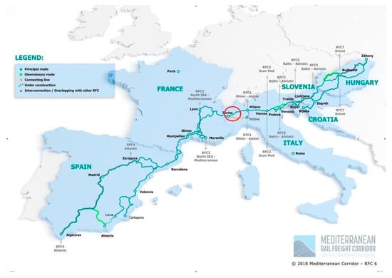
Figure 1.
The layout of Rail Freight Corridor 6, the “Mediterranean Corridor” [19]. The red circle indicates the studied segment, linking the city of Turin and the city of Novara, Northwestern Italy.
The climate of the area is temperate with an annual mean temperature ranging between 12.5 (Turin) and 12.7 °C (Novara) and average annual precipitation ranging between 809 (Turin) and 918 mm (Novara) [20]. The rainfall is not homogeneously distributed during the year, with the wettest seasons in spring and autumn.
The soils of the area originated from alluvial sediments [21] and can be mainly attributed to three different orders of the Soil Taxonomy: Alfisols, Entisols, and Inceptisols. In particular, according to the Regional Soil Map (1:250.000), most of the soils in the area were classified as Typic Udifluvents and Anthraquic Eutrudepts.
The building of the rail segment ended in February 2006, and the construction sites were restored by private companies immediately after, in order to start and accelerate secondary succession. The construction sites were used both to stock soil and inert materials and as a passage for heavy machinery that was used during the building activities. As topsoil and vegetation were removed from the construction sites, the restoration activities included the improvement of soil conditions, the sowing of an herbaceous species mixture, and the plantation of trees and shrubs. Soil restoration included three different steps:
- The gravel layer, which is normally distributed after topsoil removal to protect the substrate during the works, was removed;
- To reduce the risk of waterlogging while promoting deep rooting, rippers decompacted the substrate;
- The stockpiled soil or allochthonous topsoil was spread over the area under restoration.
Later, in the same year, trees and shrubs were planted, and herbaceous species were sowed. Information regarding the plant species used in the restoration project was collected both by restoration project documents and direct interviews with the private companies that directly carried out the fieldwork. Planting was carried out using trees and shrubs, coming from the lowland oak–hornbeam Mesophytic deciduous forest, dominated by Quercus robur L. and Carpinus betulus L. (potential climax vegetation in the Po Plain). In most of the analyzed areas, Carpinus betulus L. (hornbeam—156 plants per hectare), Fraxinus excelsior L. (ash—62 plants per hectare), Quercus robur L. (pedunculate oa—189 plants per hectare), Cornus sanguinea L. (dogwood—625 plants per hectare), Crataegus monogyna Jacq. (hawthorn—625 plants per hectare), and Euonymus europaeus L. (spindle tree—625 plants per hectare) were planted in a mixture. Data analyses were performed considering 2 groups: trees and shrubs. The seedlings were 2-year-old containerized plants, and their mean height at planting time was 50 cm. The herbaceous species mixture used in the areas was composed of 5% Dactylis glomerata L., 25% Festuca arundinacea Schreb., 5% Lolium multiflorum Lam., 10% Lolium perenne L., 5% Phleum pratense L., 20% Festuca rubra L., 10% Poa pratensis L., 5% Festuca gr. ovina L., 5% Medicago sativa L., 5% Trifolium pratense L., 5% Trifolium repens L. The restoration activities were completed in 2007.
2.2. Experimental Design and Data Collection
In 2014, 8 years after the implementation of the restoration project, we assessed the effectiveness of soil restoration, the effectiveness and naturalness of sward restoration, as well as the success of plantations.
According to the shape of the area, a circular or rectangular plot was designed (314 or 300 m2 per plot, 28 plots in total). Moreover, for soil properties and herbaceous vegetation surveys, 2 circular subplots (2 m radius) per plot were created (56 subplots in total). The 2 subplots were located along a random trajectory, 5 m away from the center of the plot (Figure 2).
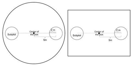
Figure 2.
Schematic representation of the sampling design. On the left is a 314 m2 circular plot. On the right is a 300 m2 rectangular plot. Two 2 m radius subplots were located inside each plot. The subplots were 5 m away from the center of the plot.
In the middle of each subplot, a soil mini-pit was dug. The total soil depth was measured by means of a hand auger. Soil aggregates were described, and soil mottling was quantified, as well as soil penetration resistance, by means of pocket penetrometer. A sample of each genetic horizon described in the field was collected for chemical and physical characterization. The upper soil horizons (generally A horizons) were named topsoil, while the deeper soil horizons (generally AC and C horizons) were defined as subsoil. All the samples were oven dried and sieved at the less than 2 mm and less than 0.5 mm fractions. The particle size distribution was determined by the pipette method. The pH was determined potentiometrically in water extracts (soil/solution = 1:2.5). The total C and N concentrations were obtained by dry combustion with an elemental analyzer (CE Instruments NA2100, Rodano, Italy). The carbonate content was measured by volumetric analysis of the carbon dioxide liberated by a 6 M HCl solution. Organic carbon (TOC) was then calculated as the difference between total C content measured by dry combustion and carbonate—C. To assess soil vulnerability to water erosion, the water aggregate stability 60 (WAS60) was measured [22]. Soil aggregate stability was determined by wet sieving at 60 min. An exponential model was used to evaluate the breakdown kinetics [22] Y(t) = a + b(1 − e−t/c), where y is the aggregate breakdown (%), t is the wet sieving time (min), b is the aggregate loss by abrasion (%), a is the incipient failure of aggregates upon water saturation (%), and c is the time-unit parameter that links the rate of breakdown to wet-sieving time.
Herbaceous species were identified at the taxonomical level of species according to [23]. The cover of each plant species with greater than 1% cover and the bare ground cover were visually estimated. Herbaceous height was measured through the “sward stick method” [24] in 5 different points per subplot. Then, each plant species was associated with its phytosociological optimum (at class level) according to [25]. This approach has been largely used to evaluate vegetation response to management and disturbance regimes in different ecosystems [26,27,28,29,30]. Plant species were pooled into 2 vegetation groups according to their phytosociological optimum to express the level of habitat naturalness:
- Native spontaneous ruderal species;
- Native spontaneous grassland species.
The first group included both annual (i.e., species belonging to the Stellarietea mediae class) and perennial plant species (species belonging to the Agropyretea intermedii-repentis and Artemisietea vulgaris classes). The second group included plant species belonging to the Molinio-Arrhenatheretea class. Then, the percentage cover of the following herbaceous species assemblages was calculated for each plot:
- Sown species;
- Total spontaneous species (i.e., the species not belonging to the sown mixture, including both native and alien species);
- Annual and perennial spontaneous species (according to [31]);
- Alien species (i.e., the cumulative cover of Ambrosia artemisifolia L., Artemisia verlotorum Lamotte, Erigeron annus (L.) Pers., Helianthus tuberosus L., Lepidium virginicum L., Oxalis fontana Bunge, Solidago gigantea Aiton., Thlaspi arvense L., Veronica persica Poiret);
- Native spontaneous species divided into ruderal species and typical grassland species (hereafter ruderal species and typical grassland species).
Ruderal and alien species were commonly spread in the soils used for the restoration, both as seeds and vegetative organs. In the 28 plots, species and height of all the plants present inside the plot (trees and shrubs) were recorded. Height was measured as the stretched length from the ground to highest located buds, using a ruler with a degree of precision of ± 1 cm. No shrubs were found in one of the 28 plots; thus, we recorded species and height of shrubs in 27 plots.
2.3. Data Analyses
In 4 of the selected areas, the herbaceous layer did not present any species from the herbaceous mixture. Areas in which it was not possible to evaluate if herbaceous species were either not sown or did not germinate were excluded from the analyses. Thus, we used data from 56 subplots to study sward restoration effectiveness and naturalness. As no trees or shrubs were found in some areas, the total number of plots analyzed for trees and shrubs was 28 and 27, respectively.
Soil properties were used in the analyses as predictors. In order to weigh the contribution of topsoil and subsoil properties in the whole mini-pit, the following formula was applied [(Ti × T) + (Sj × S)]/D, where Ti is the considered soil parameter in the topsoil, T is the depth of the topsoil, Sj is the considered soil parameter in the subsoil, S is the depth of the subsoil, and D is the soil depth. We used data collected in each pit in herbaceous vegetation analyses and the mean between the 2 pits dug in the same plot in tree and shrub analyses. Degrees of soil aggregation were reported in a range from 1 to 6 [32] (1 = loose, 2 = weak, 3 = moderate, 4 = strong, 5 = very strong, 6 = massive) while soil mottling had a range from 0 to 4 (0% = 0, <2% = 1, 2–20% = 2, 20–40% = 3, >40% = 4) The soil mottling percentage was estimated on the ped surfaces.
Soil properties were standardized (Z-scores) to analyze the size of the effect of every property by comparing model parameter estimates (β coefficients). A correlation matrix (Pearson coefficient) was used to exclude predictors with high collinearity (r > |0.70|) from the following analyses (sand and total nitrogen, TN, were excluded). In order to better explain our results, soil properties were grouped into soil physical properties (soil depth; clay, silt, sand, and rock > 2 mm content; soil mottling; soil penetration resistance; degree of soil aggregation; and WAS60) and into chemical properties of the soil (TOC, TN, C/N, and pH). Moreover, in alien, ruderal, and grassland species cover analyses, the standardized cover of the sown species was used as predictor. Standardized cover of the sown species and standardized herbaceous layer height were included among predictors in tree and shrub growth analysis. Assumptions of normality and homogeneity of variance were checked (p > 0.05) with Shapiro–Wilk and Levene’s tests, respectively. When variables were not normally distributed, arcsine or square root transformations were applied prior to performing the further statistical analyses.
Topsoil and subsoil parameters were compared using the Wilcoxon signed rank test, which can describe chemical and physical properties of soil. Since topsoil depth was limited and we supposed that in 8 years plant roots also explore deeper horizons, further analyses were performed using the properties recorded in the whole depth.
To test for the effectiveness of sward restoration:
- The correlation (Pearson coefficient) between sown and spontaneous species cover was tested;
- Wilcoxon signed rank tests were performed to look for significant differences between sown and spontaneous and annual and perennial species cover. Wilcoxon signed rank tests were used as normal distribution or homogeneity of variances were not met, even after arcsine and square root transformations;
- Beta regression was carried out to study the effects of soil parameters on total, sown, spontaneous, annual, and perennial herbaceous species cover. The species covers were expressed as a percentage, ranging from 0% to 100%. Percentages were transformed into a range from 0 to 1, in order to use the beta regression. We applied the transformation (n = sample size) to avoid 0 and 1 values, according to [33].
To test for the naturalness of sward restoration:
- The Kruskal–Wallis test was performed to look for differences in the herbaceous cover of alien, ruderal, and grassland species. Kruskal–Wallis was used as normal distribution or homogeneity of variances were not met, even after arcsine and square root transformations;
- Beta regression was run to test the effects of soil parameters on alien, ruderal, and grassland herbaceous species cover. Cover percentages were transformed as explained before.
Finally, to assess the success of the plantation:
- Mean 8-year growth was calculated for trees and shrubs;
- Wilcoxon signed rank test was performed to look for significant differences between tree and shrub mean 8-year growth;
- The effects of soil properties on tree and shrub mean 8-year growth were evaluated through general linear models (GLMs).
All tests were performed using R version 3.5.1 software [34].
3. Results
3.1. Pedological Conditions
Both physical and chemical parameters of soil showed a wide range of values between topsoil and subsoil in the study areas (Figure 3 and Figure 4, respectively) The topsoil depth was generally determined to be less than 10 cm, while subsoil was thicker, even reaching more than 50 cm. Soil texture did not show significant differences between topsoil and subsoil, with the predominance of the sand fraction. Soil mottling was more present in the subsoil. The degree of soil aggregation was generally massive in the subsoil, while a better aggregation degree was present in the topsoil, which was also less compacted than the subsoil.
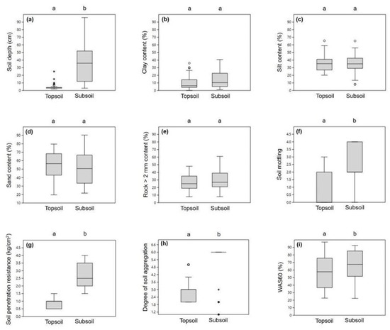
Figure 3.
Soil physical properties recorded in the study areas in the topsoil and in the subsoil. (a) soil depth (cm); (b) clay content (%); (c) silt content (%); (d) sand content (%); (e) rock >2 mm content (%); (f) soil mottling; (g) soil penetration resistance (kg/cm2); (h) degree of soil aggregation; (i) water aggregate stability 60 (WAS60; %). Different letters indicate significant differences between topsoil and subsoil (p < 0.001). Identical letters indicate no differences between topsoil and subsoil (p > 0.001). The start of the box represents the lower quartile (25%), the black line within the box the median, and the end of the box the upper quartile (75%). Hollow circles and stars represent outliers, values outside 1.5 and 3 times the interquartile range, respectively.
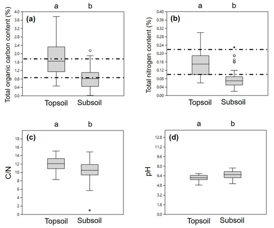
Figure 4.
Soil chemical properties recorded in the study areas in the topsoil and in the subsoil. (a) total organic carbon content—TOC (%); (b) total nitrogen content—TN (%); (c) C/N; (d) pH. The upper and lower dashed lines indicate optimum and moderate conditions for the considered soil properties, respectively. This classification has been proposed according to the guidelines for soil quality evaluation reported by Curtaz et al. (2013). Different letters indicate significant differences between topsoil and subsoil (p < 0.001). Identical letters indicate no differences between topsoil and subsoil (p > 0.001).
Moreover, in the topsoil, TOC and TN were significantly higher compared with subsoil, and the C/N ratio was higher as well. pH was higher in the subsoil.
3.2. Effectiveness of Sward Restoration
Eight years after sward restoration, the total herbaceous cover was higher than 60% in all the 56 subplots. This result was confirmed by the correlation between sown and spontaneous species (Figure 5). Areas in which sown species did not establish successfully were colonized by spontaneous species (r = −0.918; p < 0.001). Moreover, according to the Wilcoxon signed rank test, sown species cover was significantly higher than the cover of spontaneous species (p < 0.001).
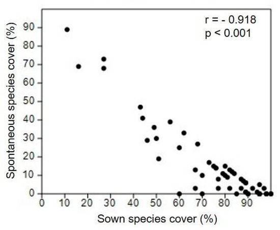
Figure 5.
Sown species cover correlation (Pearson coefficient) with spontaneous species cover. Each dot represents a single subplot (56 dots = 56 subplots). r = −0.918, p < 0.001.
A significant difference in annual and perennial species cover was found (Figure 6), the cover of perennial species being higher than the cover of annual species (p < 0.001).
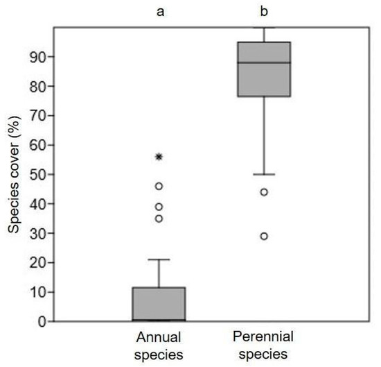
Figure 6.
Annual and perennial species cover percentage. Different letters indicate significant differences between cover percentages (p < 0.001).
Beta regressions showed that different soil parameters affected herbaceous covers (Table 1).

Table 1.
Summary of beta regression for total, sown, spontaneous, annual, and perennial herbaceous species cover. Soil properties were used as predictors. Soil properties were grouped into physical and chemical soil properties. Bold font indicates statistical significance.
The models showed that total herbaceous cover was positively affected by the soil gravel content (rocks > 2 mm) and TOC, the effect of which, according to the beta value, was the strongest. Physical properties (mainly WAS60 and soil aggregation degree) influenced sown and spontaneous species cover, with opposite effects (e.g., WAS60 positively affected sown species while negatively impacting spontaneous ones). The most important parameters for annual and perennial species were again physical properties (WAS60 and soil mottling, respectively).
3.3. Naturalness of Sward Restoration
Alien, ruderal, and typical grassland species generally reached low cover percentages, and no significant differences were shown among them (Figure 7). Moreover, any significant correlation (Pearson coefficient) amongst these three groups of species was assessed.
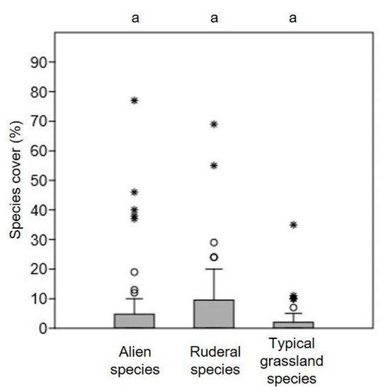
Figure 7.
Alien, ruderal, and typical grassland species cover percentage. Letters indicate no differences among cover percentages (p > 0.05).
Beta regressions indicated that sown species cover significantly reduced the cover of alien, ruderal, and typical grassland species (Table 2). Moreover, parameters that significantly affected alien and ruderal species cover, such as soil depth, silt content, soil aggregates, and pH, acted on the cover in opposite ways.
Table 2.
Summary of beta regression for alien, ruderal, and typical grassland species cover. Soil properties and sown species cover were used as predictors. Soil properties were grouped into physical and chemical soil properties. Bold font indicates statistical significance.
The most important soil parameters for alien, ruderal, and typical grassland species cover were respectively WAS60, silt content, and rock content.
3.4. Trees and Shrubs Growth
After 8 years, mean growth of trees was 1.4 m ± 0.9, while mean growth of shrubs was 0.9 m ± 0.6 (Figure 8).
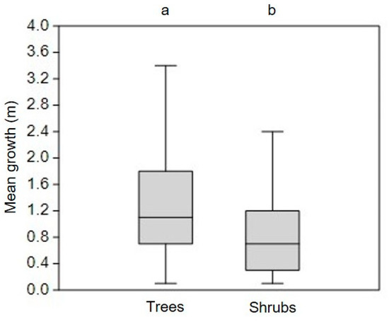
Figure 8.
Mean tree and shrub 8-year growth. Different letters indicate significant differences between the growth of trees and shrubs (p < 0.05).
GLMs showed (Table 3) that tree growth was affected by the total herbaceous species cover, while no significant effects from the herbaceous layer were shown on shrub growth. Moreover, soil properties did not influence woody species growth.
Table 3.
Summary of general linear models (GLMs) for tree and shrub mean 8-year growth. Soil properties, total herbaceous species cover, and herbaceous layer height were used as predictors. Soil properties were grouped into physical and chemical soil properties. Bold font indicates statistical significance.
4. Discussion
This study showed that soil–plant interaction differently affected vegetation group dynamics after restoration. The soil’s physical and chemical properties indicated good quality and fertility after 8 years. This result likely was a consequence of proper site preparation techniques. Soil penetration resistance was always lower than 18.3 kg/cm2, a threshold under which soil is loosened enough for plant development [35]. The levels of total organic carbon and nitrogen in the topsoil were generally greater than 0.87% and 0.1%, respectively. Thus, they were raised over the levels required by one of the Italian Regional Guidelines for anthropogenic soil recovery [36]. Rock content was usually lower than 50%, and pH was suitable for plant establishment as well [37]. The total herbaceous cover was positively influenced by the rock content, which could contribute to increase the soil porosity in these disturbed soils, while the soil organic matter had a fundamental role in influencing the soil fertility.
Fertile topsoil may have favored the development of herbaceous vegetation, the cover of which was higher than 60% in all the areas. Despite the topsoil depth never exceeding 25 cm, sown species could establish well, probably because 80% of their roots develop in the first 25–50 cm of soil [31]. An initial grass content in the seed mixture greater than 70% successfully reduced spontaneous species cover over time [38,39]. Thus, alien species, which can be a threat for the native ones, [40], usually covered less than 10% of the areas. The seed mixture was composed of species often used in commercial seed mixtures. These mixtures are able to establish fast in a wide variety of site conditions, as they include a large number of perennial generalists [41]. In our study, plant species of the mixture rapidly colonized poorer sites, where soils were more shallow, coarse, and compacted compared to soils where spontaneous species were established. Moreover, they took advantage of fewer aggregate soils, even if other authors found that graminoids improve soil aggregation through their fine roots [42]. Sown species were probably able to rapidly produce cover in poor soil, as the mixture contained species such as Festuca arundinacea, Festuca gr. rubra, and Poa pratensis, which are strong competitors and can expand through their rhizomes and outcompete spontaneous herbaceous species [43].
Eight years after the sown mixture was applied, perennial prevailed over annual herbaceous plant species, confirming the finding of [44]. Annual and perennial species, as well as sown and spontaneous ones, were established in different ecological niches. Annuals, with short life cycles, were able to spread on areas where temporary flooding may happen (with a significant positive effect on their cover from soil mottling), while perennials preferred draining soils, rich in total organic carbon, that support their long-life span [45].
Alien, ruderal, and typical grassland species generally cover less than 10% of the areas, with no significant differences among the cover percentage of the three groups. Alien species and ruderals colonized soils with opposite characteristics. Physical properties seemed to affect their establishment more than chemical ones. Aliens colonized deeper soils and were positively influenced by the degree of soil aggregation, while ruderals found space for the establishment in more shallow soils, subjected to periodic flooding. Typical grassland species of Molinio-Arrhenatheretea included several stress-tolerant plant species, which colonized sites with a higher rock content.
As alien species are usually fast colonizers, they were rapidly established on good quality soil, becoming competitors for ruderal and typical grassland species [46]. Ruderal species probably took advantage from harsher soil conditions, where competition was reduced and bare soil was present. Sown species cover negatively influenced the cover of alien, ruderal, and typical grassland species, the establishment of which was successful only when sown species development was lower. Undesired alien species were controlled by the sown mixture, while natural desired ruderal and typical grassland ones were hampered [43]. Even though sown species provided a soil cover quickly, reducing soil erosion risk, they delayed spontaneous vegetation establishment. Moreover, the absence of viable seeds in the seed bank and low seed dispersal, linked to the lack of grassland in the surrounding landscape, may have hampered spontaneous desired species expansion [47].
Tree and shrub mean growth in the eight year was 1.4 and 0.9 m, respectively, and soil properties did not significantly affect their growth. Planted species were quite exigent in term of soil and microhabitat, as they were typical of late successional vegetation. Even if in natural secondary succession woody species can appear before the eighth year, they are usually pioneer species, e.g., Betula pendula and Salix caprea [48]. Late-successional species usually establish after pioneer ones, when soil and microclimatic conditions are improved, for example, thanks to the shadow produced by canopies and thanks to the litter that improves soil organic matter content [49]. Wrong initial species selection may have influenced forest restoration. Natural regeneration potential may have been taken into account to understand whether the selected species were suitable for the degraded site conditions or not [50]. Even if in our study areas soil was suitable for herbaceous species development, woody species probably needed a more fertile substrate.
The herbaceous cover seemed to facilitate tree growth, contrary to other authors’ findings. Indeed, it has been demonstrated that an herbaceous cover of 50% reduced photosynthetically active radiation by 50%, being a competitor for light [51]. Moreover, the dense herbaceous cover can also compete for nutrients and moisture, delaying tree establishment and reducing height growth [52,53]. However, plant–plant interactions are affected by several factors, such as microclimatic conditions, stressors, and plant physiological traits [54]. Some form of facilitation may have occurred in our experiments. For instance, herbaceous species with deep roots could have transported water from deeper and wetter layers of soil into shallower and drier ones through the “hydraulic lift”, allowing trees to grow better [55].
5. Conclusions
Eight years after restoration, in our study areas, physical and chemical properties of soil were suitable to support sowing and planting. The sown herbaceous mixture was the key to success for sward restoration. Herbaceous cover was generally high in all areas, with perennial plant species prevailing over annuals. Moreover, sown species efficiently limited the development of alien undesired species. Contrarily, they also hampered the establishment of ruderal and typical grassland species, the presence of which may improve sward naturalness. The plantation of late seral woody species in the early stage of secondary succession led to a reduction in tree and shrub growth. Soil properties did not influence sapling performance, probably because microclimatic conditions of the areas were unsuitable for exigent species development.
Together, our results highlighted that proper evaluation of the restoration techniques is necessary to reach the target goal. In order to improve restoration success, follow-up monitoring has to be carried out, as it helps in adjusting restoration activities. The time factor, which implies constant and prolonged monitoring and maintenance, is crucial for the success of the restoration process. It is therefore unlikely that the ecosystem can recover enough in the immediate future to provide functions comparable to natural ones. However, with an appropriate restoration strategy, these areas, although artificial, may represent new habitats able to sustain biodiversity and provide an increase in other ecosystem services.
Author Contributions
Conceptualization, F.M., M.F. (Michele Freppaz), M.L. and M.F. (Massimiliano Ferrarato); Data curation, S.M., M.F. (Michele Freppaz), M.L. and M.P.; Investigation, F.M., A.P. and M.L.; Methodology, F.M., M.F. (Michele Freppaz), M.L. and M.F. (Massimiliano Ferrarato); Writing—original draft, S.M., M.F. (Michele Freppaz), M.L. and M.P.; Writing—review & editing, F.M., A.P., M.F. (Massimiliano Ferrarato), R.M. and A.N. All authors have read and agreed to the published version of the manuscript.
Funding
This research received no external funding.
Conflicts of Interest
The authors declare no conflict of interest.
References
- SER—Society for Ecological Restoration International Science and Policy Working Group. The SER International Primer on Ecological Restoration; Society for Ecological International: Tucson, AZ, USA, 2004; Available online: www.ser.org (accessed on 19 December 2019).
- Miller, J.R.; Hobbs, R.J. Habitat restoration—Do we know what we’re doing? Restor. Ecol. 2007, 15, 382–390. [Google Scholar] [CrossRef]
- Aradottir, A.L.; Hagen, D. Chapter three—Ecological restoration: Approaches and impacts on vegetation, soils and society. Adv. Agron. 2013, 120, 173–222. [Google Scholar] [CrossRef]
- Halme, P.; Allen, K.A.; Auniņš, A.; Bradshaw, R.H.W.; Brūmelis, G.; Čada, V.; Clear, J.L.; Eriksson, A.; Hannon, G.; Hyvärinen, E.; et al. Challenges of ecological restoration: Lessons from forests in northern Europe. Biol. Conserv. 2013, 167, 248–256. [Google Scholar] [CrossRef]
- Costantini, E.A.C.; Branquinho, C.; Nunes, A.; Schwilch, G.; Stavi, I.; Valdecantos, A.; Zucca, C. Soil indicators to assess the effectiveness of restoration strategies in dryland ecosystems. Soild Earth 2016, 7, 397–414. [Google Scholar] [CrossRef]
- Vallauri, D.; Aronson, J.; Dudley, N.; Vallejo, R. Monitoring and evaluating forest restoration success. In Forest Restoration in Landscapes; Springer: New York, NY, USA, 2005. [Google Scholar] [CrossRef]
- Zedler, J.B.; Callaway, J.C. Tracking wetland restoration: Do mitigation sites follow desired trajectories? Restor. Ecol. 1999, 7, 69–73. [Google Scholar] [CrossRef]
- Tischew, S.; Baasch, A.; Conrad, M.K.; Kirmer, A. Evaluating restoration success of frequently implemented compensation measures: Results and demands for control procedures. Restor. Ecol. 2010, 18, 467–480. [Google Scholar] [CrossRef]
- Ruiz-Jaén, M.C.; Aide, T.M. Restoration success: How is it being measured? Restor. Ecol. 2005, 13, 569–577. [Google Scholar] [CrossRef]
- Wortley, L.; Hero, J.; Howes, M. Evaluating ecological restoration success: A review of the literature. Restor. Ecol. 2013, 21, 537–543. [Google Scholar] [CrossRef]
- Ruiz-Jaén, M.C.; Aide, T.M. Vegetation structure, species diversity, and ecosystem processes as measures of restoration success. For. Ecol. Manag. 2005, 218, 159–173. [Google Scholar] [CrossRef]
- Defra—Department of Environment, Food and Rural Affairs. Construction Code of Practice for the Sustainable use of Soils on Construction Sites; Defra—Department of Environment, Food and Rural Affairs: London, UK, 2009.
- Schoenholtz, S.H.; Van Miegroet, H.; Burger, J.A. A review of chemical and physical properties as indicators of forest soil quality: Challenges and opportunities. For. Ecol. Manag. 2000, 138, 335–356. [Google Scholar] [CrossRef]
- Cogger, C.G. Potential compost benefits for restoration of soils disturbed by urban development. Compost Sci. Util. 2005, 13, 243–251. [Google Scholar] [CrossRef]
- Löf, M.; Dey, D.C.; Navarro, R.M.; Jacobs, D.F. Mechanical site preparation for forest restoration. New For. 2012, 43, 825–848. [Google Scholar] [CrossRef]
- Heneghan, L.; Miller, S.P.; Baer, S.; Callaham, M.A., Jr.; Montgomery, J.; Pavao-Zuckerman, M.; Rhoades, C.C.; Richardson, S. Integrating soil ecological knowledge into restoration management. Restor. Ecol. 2008, 16, 608–617. [Google Scholar] [CrossRef]
- Haan, N.L.; Hunter, M.R.; Hunter, M.D. Investigating predictors of plant establishment during roadside restoration. Restor. Ecol. 2012, 20, 315–321. [Google Scholar] [CrossRef]
- European Commission. 2018. Available online: https://ec.europa.eu/transport/themes/infrastructure/mediterranean_en (accessed on 18 December 2019).
- Mediterranean Rail Freight Corridor. 2020. Available online: https://www.railfreightcorridor6.eu/RFC6/web.nsf/OnePager/index.html (accessed on 24 April 2020).
- Perosino, G.C.; Zaccara, P. Elementi climatici del Piemonte; CREST—Centro Ricerche in Ecologia e Scienze del Territorio: Torino, Italy, 2006. [Google Scholar]
- Carta dei Suoli del Piemonte. 2019. Available online: http://www.sistemapiemonte.it/cms/privati/agricoltura/servizi/383-carta-dei-suoli-1-50-000 (accessed on 15 December 2019).
- Zanini, E.; Bonifacio, E.; Albertson, J.D.; Nielsen, D.R. Topsoil aggregate breakdown under water-saturated conditions. Soil Sci. 1998, 163, 288–298. [Google Scholar] [CrossRef]
- Pignatti, S. Flora d’Italia; Voll. 1-2-3; Ed agricole: Bologna, Italy, 1982. [Google Scholar]
- Stewart, K.E.J.; Bourn, N.A.D.; Thomas, J.A. An evaluation of three quick methods commonly used to assess sward height in ecology. J. Appl. Ecol. 2001, 38, 1148–1154. [Google Scholar] [CrossRef]
- Aeschimann, D.; Lauber, K.; Moser, D.M.; Theurillat, J.P. Flora Alpina: Atlante delle 4500 Piante Vascolari delle Alpi; Zanichelli: Bologna, Italy, 2004. [Google Scholar]
- Lonati, M.; Vacchiano, G.; Berretti, R.; Motta, R. Effect of stand-replacing fires on Mediterranean plant species in their marginal alpine range. Alp. Bot. 2013, 123, 123–133. [Google Scholar] [CrossRef][Green Version]
- Moris, J.V.; Vacchiano, G.; Ravetto Enri, S.; Lonati, M.; Motta, R.; Ascoli, D. Resilience of European larch (Larix decidua Mill.) forests to wildfires in the western Alps. New For. 2017, 48, 663–683. [Google Scholar] [CrossRef]
- Orlandi, S.; Probo, M.; Sitzia, T.; Trentanovi, G.; Garbarino, M.; Lombardi, G.; Lonati, M. Environmental and land use determinants of grassland patch diversity in the western and eastern Alps under agro-pastoral abandonment. Biodivers. Conserv. 2016, 25, 275–293. [Google Scholar] [CrossRef]
- Pittarello, M.; Probo, M.; Lonati, M.; Lombardi, G. Restoration of sub-alpine shrub-encroached grasslands through pastoral practices: Effects on vegetation structure and botanical composition. Appl. Veg. Sci. 2016, 19, 381–390. [Google Scholar] [CrossRef]
- Vacchiano, G.; Meloni, F.; Ferrarato, M.; Freppaz, M.; Chiaretta, G.; Motta, R.; Lonati, M. Frequent coppicing deteriorates the conservation status of black alder forests in the Po plain (northern Italy). For. Ecol. Manag. 2016, 382, 31–38. [Google Scholar] [CrossRef]
- Landolt, E.; Bäumler, B.; Erhardt, A.; Hegg, O.; Klötzli, F.; Lämmler, W.; Nobis, M.; Rudmann-Maurer, K.; Schweingruber, F.H.; Theurillat, J.P.; et al. Flora Indicativa: Ökologische Zeiterwerte Und Biologische Kennzeichen Zur Flora Der Schweiz Und Der Alpen=Ecological Indicator Values and Biological Attributes of the Flora of Switzerland and the Alps; Editions des Conservatoire et Jardin botaniques de la Ville de Genève & HauptVerlag: Bern, Switzerland; Stuttgart, Germany; Vienna, Austria, 2010. [Google Scholar]
- FAO. 2019. Available online: http://www.fao.org/fishery/static/FAO_Training/FAO_Training/General/x6706e/x6706e07.htm (accessed on 15 December 2019).
- Cribari-Neto, F.; Zeileis, A. Beta Regression in R. Research report series/Department of Statistics and Mathematics, 98; Department of Statistics and Mathematics, WU Vienna University of Economics and Business: Vienna, Austria, 2009. [Google Scholar]
- R Core Team. R: A Language and Environment for Statistical Computing; R Foundation for Statistical Computing: Vienna, Austria, 2018. [Google Scholar]
- Young, D.; van Seters, T. Preserving and Restoring Healthy Soil: Best Practices for Urban Construction; Toronto and Region Conservation Authority: Toronto, ON, Canada, 2012. [Google Scholar]
- Curtaz, F.; Filippa, G.; Freppaz, M.; Stanchi, S.; Zanini, E.; Costantini, E.A.C. Guida Pratica di Pedologia: Rilevamento di Campagna, Principi di Conservazione e Recupero dei Suoli; Istitut Agricole Régional, Rég. La Rochère: Aosta, Italy, 2013. [Google Scholar]
- Sheoran, V.; Sheoran, A.S.; Poonia, P. Soil reclamation of abandoned mine land by revegetation: A review. Int. J. Soil Sediment Water 2010, 3, 13. [Google Scholar]
- Van der Putten, W.H.; Mortimer, S.R.; Hedlund, K.; Van Dijk, C.; Brown, V.K.; Lepš, J.; Rodriguez-Barrueco, C.; Roy, J.; Diaz Len, T.A.; Gormsen, D.; et al. Plant species diversity as a driver of early succession in abandoned fields: A multi-site approach. Oecologia 2000, 124, 91–99. [Google Scholar] [CrossRef] [PubMed]
- Lepŝ, J.; Doleẑal, J.; Bezemer, T.M.; Brown, V.K.; Hedlund, K.; Igual Arroyo, M.; Jörgensen, H.B.; Lawson, C.S.; Mortimer, S.R.; Peix Geldart, A.; et al. Long-term effectiveness of sowing high and low diversity seed mixtures to enhance plant community development of ex-arable fields. Appl. Veg. Sci. 2009, 10, 97–110. [Google Scholar] [CrossRef]
- D’Antonio, C.; Meyerson, L.A. Exotic plant species as problems and solutions in ecological restoration: A synthesis. Restor. Ecol. 2002, 10, 703–713. [Google Scholar] [CrossRef]
- Conrad, P.J. Effectiveness and Costs of Measures for the Establishment of Species-Rich Grasslands: Development and Application of Procedure for Efficiency Controls. In Proceedings of the 7th European Conference on Ecological Restoration 2010, Avignon, France, 23–27 August 2010; Available online: http://opus.kobv.de/tuberlin/volltexte/2007/1550/ (accessed on 18 December 2019).
- Pohl, M.; Stroude, R.; Buttler, A.; Rixen, C. Functional traits and root morphology of alpine plants. Ann. Bot. 2011, 108, 537–545. [Google Scholar] [CrossRef]
- Conrad, M.K.; Tischew, S. Grassland restoration in practice: Do we achieve the targets? A case study from Saxony-Anhalt/Germany. Ecol. Eng. 2011, 37, 1149–1157. [Google Scholar] [CrossRef]
- Török, P.; Matus, G.; Papp, M.; Tóthmérész, B. Secondary succession in overgrazed Pannonian sandy grasslands. Preslia 2008, 80, 73–85. [Google Scholar]
- Grime, J.P. Plant Strategies, Vegetation Processes, and Ecosystem Properties; John Wiley & Sons: West Sussex, UK, 2006. [Google Scholar]
- DeFalco, L.A.; Bryla, D.R.; Smith-Longozo, V.; Nowak, R.S. Are Mojave desert annual species equal? Resource acquisition and allocation for the invasive grass Bromus madritensis subsp. rubens (Poaceace) and two native species. Am. J. Bot. 2003, 90, 1045–1053. [Google Scholar] [CrossRef]
- Gaujour, E.; Amiaud, B.; Mignolet, C.; Plantureux, S. Factors and processes affecting plant biodiversity in permanent grasslands. A review. Agron. Sustain. Dev. 2012, 32, 133–160. [Google Scholar] [CrossRef]
- Prach, K. Spontaneous succession in Central-Europe man-made habitats: What information can be used in restoration practice? Appl. Veg. Sci. 2003, 6, 125–129. [Google Scholar] [CrossRef]
- Cortina, J.; Maestre, F.T.; Vallejo, R.; Baeza, M.J.; Valdecantos, A.; Pérez-Devesa, M. Ecosystem structure, function, and restoration success: Are they related? J. Nat. Conserv. 2006, 14, 152–160. [Google Scholar] [CrossRef]
- Meli, P.; Martínez-Ramos, M.; Rey-Benayas, J.M.; Carabias, J. Combining ecological, social and technical criteria to select species for forest restoration. Appl. Veg. Sci. 2014, 17, 744–753. [Google Scholar] [CrossRef]
- Rizza, J.; Franklin, J.; Buckley, D. The influence of different ground cover treatments on the growth and survival of tree seedlings on remined sites in eastern Tennesse. In Proceedings of the 24th Annual Meeting of the ASMR, Gillette, WY, USA, 2–7 June 2007; pp. 663–677. [Google Scholar]
- Prach, K.; Pyšek, P. Using spontaneous succession for restoration of human-disturbed habitats: Experience from Central Europe. Ecol. Eng. 2001, 17, 55–62. [Google Scholar] [CrossRef]
- Franklin, J.A.; Zipper, C.E.; Burger, J.A.; Skousen, J.G.; Jacobs, D. Influence of herbaceous ground cover on forest restoration of eastern US coal surface mines. New For. 2012, 43, 905–924. [Google Scholar] [CrossRef]
- Holmgren, M.; Scheffer, M.; Huston, M.A. The interplay of facilitation and competition in plant communities. Ecology 1997, 78, 1966–1975. [Google Scholar] [CrossRef]
- Armas, C.; Kim, J.H.; Bleby, T.M.; Jackson, R.B. The effect of hydraulic lift on organic matter decomposition, soil nitrogen cycling, and nitrogen acquisition by a grass species. Oecologia 2012, 168, 11–22. [Google Scholar] [CrossRef]


© 2020 by the authors. Licensee MDPI, Basel, Switzerland. This article is an open access article distributed under the terms and conditions of the Creative Commons Attribution (CC BY) license (http://creativecommons.org/licenses/by/4.0/).