Abstract
The financial penetration accelerated by economic globalization and financial liberalization has inevitably induced market co-movement and the rising likelihood of cross-market risk contagion. An in-depth analysis concerning the carrier of risk contagion, i.e., market connectedness network, is of great significance for risk management. This study aims to establish a holistic framework to shed light on the topological dynamics and the evolving channels of connectedness network among 24 major stock markets in two aspects; namely, a dynamic perspective juxtaposing crisis and non-crisis periods, and a contrasting perspective between risk absorption and risk spillover. To this end, a methodological framework of the generalized variance decomposition and generalized exponential random graph models (GERGM) is constructed, in which the former method formulates the asymmetric causal relationships of stock return volatility among countries and regions into weighted and directed networks, and the latter method simulates and models the varying attributes of different contagion channels in the formation of tie directions and weights. The results indicate that the global stock market network reflects typical event-driven and time-varying characteristics. Countries and regions that rely heavily on foreign direct investment (FDI) are more likely to absorb risks, especially during the post-crisis recovery period, while countries and regions with higher foreign portfolio holdings are more inclined to risk spillover, especially during the subprime crisis. Geographical proximity and bilateral trade volume amplify risk contagion, whereas foreign exchange reserve holding improves robustness. This holistic framework allows the identification of the direction and intensity of risk contagion and the clarification of priority of risk transmission channels in different stages, thus reducing the uncertainty of risk management and providing insights into the macro-prudential managements toward sustainable economic development.
1. Introduction
Economic globalization and financial liberalization, accompanied by the accelerated international capital flows, cross-border investments and speculative activities, have transformed the global stock markets from a state of fragmentation into a state of mutual influence and overall movement. The increasing financial penetration among countries has proven to be double-edged, which not only assists in the optimization of investment portfolios and reduction of local risks, but also induces market co-movements and consequently raises the likelihood of risk contagion across economies [1]. The repercussions of contagion are at the core of systemic risk, which depends considerably on the carrier of connectedness among financial institutions or financial markets [2,3]. Especially the recent financial crises have highlighted the role of market connectedness in triggering systemic risk [4]. An in-depth analysis of market connectedness (e.g., volatility) and its channels is of great significance in managing systemic risks and maintaining financial stability, thus contributing to the smooth functioning of the real economy in turn [5]. In this context, this study establishes a holistic framework, encompassing volatility spillover analyzing framework and the recent development of graph dependence theory, to seek a better understanding of market connectedness from a dynamic perspective. More specifically, we address the following two issues: (1) Examining the time-varying attributes of the market connectedness network by separating the dynamics of shock transmissions during crisis periods and non-crisis periods; (2) exploring the relative importance of various influencing channels in shaping the dynamics of the market interdependence.
The study relates to two main lines of literature. One stream of literature focuses on financial networks. The inner logic of financial networks is that the intricate connectedness, either physical based on bilateral exposures/flows between financial institutions, or association-based depicting return dependency among financial markets, could be captured and analyzed in complex financial systems using a network approach [1,2,6]. The network approach, which describes relationship architecture and regularities involved in complex multivariate systems, has become a powerful tool in financial crises early warning and tracking [7,8], risk spillover sources tracing [9,10], or exploitation of asset allocation [11,12]. Three research paradigms exist in the current financial network literature [1], namely, (i) mean-spillover network or Granger-causality network [13], (ii) volatility spillover network represented by variance decomposition-based network [14] and GARCH-based network [15], and (iii) risk spillover network with the main forms in tail-risk driven network [16] and extreme risk network [8]. These three overarching frameworks have enlightened many empirical works. For example, Papana et al. [17] built Granger-causality networks to conduct connectivity analyses of 21 international stock indices. Mensi et al. [18] built volatility spillover networks of global, regional and GIPSI stock market by drawing on the Diebold and Yilmaz [14] methodology. Zhang et al. [5] applied GARCH-BEKK model to construct volatility networks of the G20 stock market. These studies demonstrate the feasibility and versatility of econometric-based networks in capturing financial network topology, volatility spillover, and risk contagion mechanisms.
Referring to previous work, our study focuses on the volatility spillovers, which are generally measured by two means: the GARCH family models and Diebold and Yilmaz [14,19] spillover index method (hereafter DY2014). In this study, we employ DY2014 to examine the connectedness network across different markets. The reasons are twofold. Methodologically, the DY2014 measures connectedness from both cross-variable dependence captured in VAR coefficients and shock dependence captured in the VAR disturbance covariant matrix, enabling the pair-wise and system-wide measurement of connectedness [19,20]. Substantially, DY2014, which renders a straightforward measurement of magnitude and direction of connectedness, is intimately linked with modern network theory in terms of overall network topology and the degree of distribution [19]. These features make DY2014 fit into the integrated analyzing framework in our study in that the volatility spillover among stock markets is treated as a weighted and directed network for both topology analysis and channels mapping of risk sending and absorption.
Another strand of literature, which addresses the second research question, relates to the quantification of the spillover channels across markets. Scholars seek to explain the influential factors that amplify or mitigate volatility spillover in terms of equity market importance, development and liquidity [10,21,22,23], investment behaviors and macroeconomic fundamentals [1,20], capital account flow [24,25], financial crisis [20,26,27], and financial institution linkages [3,28]. For instance, Baumöhl et al. [10] used spatial regression to model the volatility spillover network of 40 developed, emerging, and frontier stock markets between 2006 and 2014 to identify escalating magnitude of spillovers with increasing market size, market liquidity, and economic openness. Applying the same method in the G20 stock network, Zhang et al. [1] found that government debt and inflation are positively correlated with spillover risk. Most of the existing literature uses linear regression, ordinary panel regression, and spatial autoregressive models, which do not deal with the correlation problem embedded in relational data [5]. One exception is a recent analysis by Zhang et al. [5], which used the QAP method (quadratic assignment procedure) to exploit the relevance of relational data in explaining volatility spillover.
The contribution of this study is twofold. On the one hand, we construct a holistic framework by combining generalized variance decomposition and the generalized exponential random graph model (hereafter GERGM) to shed light on the characteristics and channels of stock market connectedness in two aspects: a dynamic perspective juxtaposing crisis and non-crisis periods, and a contrasting perspective between risk absorption and risk spillover. The advantage of GERGM is that it takes account of relational data and network endogeneity simultaneously while inferring spillover channels. Our unified research framework would extend the existent financial network literature methodologically, given that the majority of the current studies do not address relational data appropriately. On the other hand, our analyzing framework provides a flexible way to test the volatility spillover channels derived from theoretical models absent in the context of network analysis, such as the portfolio rebalancing theory proposed by Kodres and Pritsker [24]. In this study, the capital account channels, trade matrix, geographic matrix and macroeconomic fundamentals are taken into consideration to simulate and model stock market dependency. Therefore, unique results of financial network relative to the former econometric studies could be contrasted and revealed to present new theoretical horizons for scholars using network data.
The paper continues with a description and development of the models used to examine the presence and working mechanisms of volatility spillover in Section 2. The results of the time-varying characteristics and determinants of risk spillover and absorption are reported in Section 3, while Section 4 concludes the article.
2. Methodology
2.1. Datasets
This article selects representative stock indexes from 24 countries or regions in the world as the sample, including Australia AORD, Austria ATX, Brazil BVSP, Canada GSPTSE, China SSEC, France CAC40, Germany DAX30, Greece ASE, Hong Kong HIS, India BSE30, Ireland ISEQ, Italy FTSEMIB, Japan N225, Korea KOSPI, Luxembourg LUXX, Netherlands AEX, Norway OSEAX, Russia RTS, Spain SMSI, Sweden OMXSPI, Switzerland SSMI, Thailand SETI, United Kingdom FTSE, and United States S&P 500. The sample period is from 5 January 2004 to 30 December 2015. The data studied in this paper are retrieved from the Wind Information and RESSET Database, which provide daily closing prices of stock market indexes in 24 countries or regions. Due to the differences in holidays and suspension systems in different countries, some trading days have inconsistencies. In this regard, non-overlapping samples are deleted. In terms of the influencing factors of risk contagion, data of exchange reserve, external debt, FDI, and foreign portfolio investment from 2004 to 2015 are retrieved from the CEIC database (https://www.ceicdata.com/en). The CEIC database which represents a consensus and is an authoritative global economic data provider provides global macroeconomic and industry time series data.
2.2. Connectedness Network Construction Based on Generalized Variance Decomposition
This study is based on the construction of connectedness networks, and then we examine the time-varying attributes of the stock connectedness networks. Specifically, we use the generalized variance decomposition method based on the VAR model to formulate the asymmetric causal relationships of stock return volatility among 24 major stock markets into weighted and directed networks.
2.2.1. The VAR
The p-th order VAR, called the VAR (p) model, can be written as:
which can be simplified as:
where represents the i-th lag of , which is the stock return volatility of k countries or regions (here k = 24). c is the constant vector, and is the time-invariant coefficient matrix. ) is the vector of error terms satisfying , which indicates that there is no correlation across time for any non-zero .
To further simplify, if the VAR model does not consider exogenous variables, it is the unrestricted VAR, which can be expressed as:
or
where is the parameter matrix of the lag operator. If the root of the determinant is outside the unit circle, Equation (4) satisfies stability and can be expressed in the form of infinite moving-average as:
where satisfies
2.2.2. Generalized Variance Decomposition
Based on Equation (4) derived from the VAR model, we use the generalized variance decomposition to calculate the directional correlation coefficient between the stock market volatilities in different periods (forward W steps).
Traditionally, variance decompositions analyze the contribution of each structural shock to the changes in endogenous variables. Based on Cholesky’s variance decomposition [29], we can sum up all the historical effects of the j-th structural shock on stock volatility as the following:
where is the element of row i and column j of matrix in Equations (5) and (6). On the premise that {} has no correlation, we can use the second central moments expressed in the following terms:
to calculate the variance of :
The variance of represents the total structure shock of . In this process, the first variable is affected only by its own innovation, the second one is affected by the first and second variables, and so on. That is, the result of identification based on Cholesky decomposition depends on the ordering of variables.
However, the generalized variance decomposition (GVD) method proposed by Diebold and Yılmaz [14] treats each variable as “the first”. The results obtained by this method have nothing to do with the ordering of the variables, which is more robust. The following equation is used to measure the i-th variable’s W-step (the number of periods of variance decomposition) prediction error variance from the impact of the j-th variable, that is,where i ≠ j:
In Equation (10) which calculates , as representing the (directed) spillover index from j to i, is the standard deviation of the j-th component of ; is the selection vector with all zeros except when the element is 1; is the coefficient matrix in Equation (6), and ∑ is the covariance matrix of the error term vector or shock vector.
For normalization, we base the generalized connectedness indexes not on , but rather on where and . Then we can greatly simplify the analysis of the generalized correlation indexes.
We establish the connectedness matrix based on all volatility spillover indexes, as shown in Table 1. Specifically, in the correlation matrix, the variables in the first row represent the origin of the risk, and the variables in the first column represent the recipients of the risk. The elements of the above matrix are obtained based on the variance solution, which is used to characterize the degree of correlation between the two countries/regions.

Table 1.
Connectedness matrix.
Additionally, we define the pairwise correlation from j to i as:
In the column where the matrix From Others is located, each element in this column is the sum of the non-diagonal elements in its row. It is the sum of the volatility spillover effects of other markets on sector i, indicating the degree of correlation of other markets to sector i. The absorption index of the spillover effects of global stock market contagion could be expressed as the following:
Additionally, in the row where the matrix To Others is located, each element in the row is the sum of the non-diagonal elements in its column. It represents the sum of the impact of sector j on other sectors, and the overall relevance of sector j to its market. The spillover index of the spillover effects could be expressed as the following:
Then, the net total correlation index is defined as the following to indicate the total contagion balance of each country/region:
Finally, we use the sum of the off-diagonal items to represent total connectedness, which is formed as:
In terms of data selection and processing, we select historical price data of the stock markets of 24 countries or regions around the world as a sample. Then we divide the sample data into different periods, calculate the week volatility of index prices, and analyze the spillover effects of financial risk in the international stock market based on the above process.
2.3. GERGM Construction
Next, we explore the relative importance of various influencing factors in shaping the volatility spillover networks. Specifically, we use GERGM to deal with the continuous valued edge network based on the generalized variance decomposition, that is the matrix , in order to reveal the internal structures and external factors that affect risk absorption and spillover through model simulation and parameter estimation.
2.3.1. GERGM Conceptualization
An important measure of network statistical inference is the exponential random graph model (ERGM). Suppose that is a directed n-vertex network (adjacent matrix), where represent the total number of nodes and directed edges in this network, respectively. ERGM model of the network Y is designated as:
where θ is the parameter vector, h(Y) is the statistical vector calculated on the network, which can capture the impacts of exogenous covariates and the interdependent structure of connectedness network such as reciprocity. is the probability of the network which can be observed in all possible network permutations when given the network statistical information.
ERGM is limited to networks with binary ties. To fit the observed network having continuous-valued edges, the generalized ERGM (GERGM) is proposed which has a generalized exponential form and is similar to the logistic regression. The goodness of fit of the GERGM can be evaluated by comparing the statistical values of the simulated random network with the observed network statistics.
The process of generating probability distribution for the observed structure y relies on two different steps. Here, the n-node network with real-valued edge weights is the volatility spillover matrix between the stock markets based on the generalized variance decomposition in Section 2.1, in which n = 24, standing for the 24 stock indexes of the 24 countries/regions mentioned before.
In the first step, the joint distribution capturing the interdependence and structure of is specified on the restricted network . Compared with , the vertices of are the same as , but the edge values of are bounded and continuous between 0 and 1 (). Adjusting the ERGM formula is necessary to define the probability distribution of , and ensure the denominator is convergent. The probability distribution of is specified by the probability density function (pdf) in the following term:
where remains as a parameter vector, and is the transpose of . The function represents the joint characteristics of in the distribution of . The statistic is ensured to be finite in , and h(·) is to capture the generative structure and dependent relationships by summing the subgraph products, especially when edges are within unit intervals. For example, if our volatility spillover networks are generated by strong bilateral linkages and nodes’ preference in connecting to nodes with a higher risk outdegree, the simulated networks are likely to present high values of the “out two-stars” and “mutual dyads” statistics.
The second step is to convert the network into the support of the network by using a parameterized, and monotonically non-decreasing transformation, which is defined as the function . Specifically, the is defined as:
where is the parameter of the transformation to capture the marginal attributes of . Besides, if the network edges of are bounded between , it can be transformed by .
By the transformation of the restricted network , GERGM keeps the basic strength and structure of the ERGM, and vector h remains the flexibility of the ERGM which is rather designed on the transformed network than the network . Given that , the nature of multivariate transformations indicates the distribution of can be represented by with the transformation function, expressed in the following term:
where is the Jacobian matrix, meaning the first partial derivatives matrix as well as a diagonal matrix, so that the probability density function (pdf) of can also be written as:
where represents the monotonic transformation of the network from to [0,1], and . The choice of transformation function is very flexible, but it is advised to be an inverse cumulative distribution function (CDF) [30], which provides several benefits for research. First, when is an inverse CDF, any is a marginal pdf. In addition, when θ = 0, degenerates into a product of marginal pdfs {}, and a cross-edge weight distribution model with dyadic interdependence is obtained. The function is the statistical vector calculated on the restricted network which is used to capture exogenous effects and endogenous structures and define the probability distribution of the network. includes parameters from three aspects: structural features: ; exogeneous matrix: and ; and node attributes:, , , . To be specific, means the structural dependent features including mutual dyads, in-2-stars structure and out-2-stars structure. Both in-2-stars and out-2-stars describe the 2-stars structures, which are defined to measure the dependent nodes’ preference in connecting to nodes. Mutual dyads calculates the mutuality between two nodes (stock markets) in the form of , where function m could be “min” for or “product” for , and so on. All these features are designed to mine the smallest interaction structure and the effects among network nodes. For the exogeneous matrix, we choose the geographical distance matrix and the bilateral trade matrix to explain the impacts of exogenous linkage matrix on the interactions between networks. Concerning node covariates, we choose the covariates , , , and to represent exchange reserves, external debts, foreign direct investment (FDI) and foreign portfolio investment (FPI), respectively. The data frequency of these covariates is initially inconsistent since some are annual statistics and some are quarter statistics. To address this issue, we average the quarterly data to keep the data frequency consistent.
2.3.2. GERGM Hypotheses
We considered the factors influencing the evolution of the volatility spillover networks from the perspectives of the endogenous structure, node attributes, and exogenous networks. We propose the following hypotheses based on the previous literature.
Previous studies have shown that the efficiency of risk flows (spillover or absorption) is greater under conditions of mutuality [22]. Therefore, we propose the following hypothesis.
Hypothesis 1 (H1).
Risk contagion relationships are inclined to be mutual.
One characteristics of risk contagion is the tremendous effects exerted by origin country [31]. It implies that nodes are inclined to connect to nodes with a higher risk outdegree, that is, the networks exhibit high values of the “out two-stars” statistic. Comparatively, a significant “in two-stars” configuration will be indicative of the existence of concentrated nodes vulnerable to risk absorption. Therefore, we propose the following:
Hypothesis 2 (H2).
There exists a giant risk disseminator and a risk absorber in risk contagion networks.
Hypotheses 1 and 2 correspond to the endogenous structural variables.
Adequate exchange reserves can be regarded as a buffer against fluctuations in international payments, ensuring that countries can calmly cope with sudden financial crisis and curb financial fluctuations [32]. Therefore, we assume that exchange reserves have a negative effect on the financial turbulence of various countries.
Hypothesis 3 (H3).
Exchange reserves suppress the risk spillover and absorption effect.
Although external debt is conducive to adjusting the domestic industrial structure and making up for the insufficiency of construction funds [33], it affects risk contagion from two perspectives. On the one hand, the higher the proportion of a country’s external debt, the more likely it is to trigger risk due to the insolvency of the debt [34]. On the other hand, countries with a large burden of external debt are more vulnerable to financial shocks due to reduced export income and increased insolvency risk [35].
Hypothesis 4 (H4).
External debt affects risk absorption and risk spillover.
The financial channel is one of the main channels of risk contagion [36]. Longstaff [37] and Yuan [38] concluded that the flow of capital in financial markets had a significant impact on the creation of liquidity crises. Therefore, the foreign direct investment (FDI) is assumed to affect the evolution of the risk contagion during different periods.
Hypothesis 5 (H5).
The amount of foreign direct investment (FDI) has a bearing on risk contagion.
Foreign portfolio investment (FPI) is one of the important channels for absorbing foreign capital, and investors will adjust FPI in times of crisis according to the theory of portfolio selection [39], so securities markets (such as the trading of equity and debt) are highly volatile and liquid. We therefore assume that the country or region with more FPI is more inclined to risk spillover and absorption.
Hypothesis 6 (H6).
The amount of foreign portfolio investment (FPI) exerts influence on risk contagion.
Hypotheses 3–6 refer to nodal attributes.
Geographically close countries are often closely linked and have similar national conditions [40]. Therefore, it is assumed that the closer the geographical distance, the more obvious the risk contagion between countries
Hypothesis 7 (H7).
Geographical distance has a negative correlation with risk contagion.
Gorea and Radev [41] and Gerlach and Smets [42] have shown that the trade channel is one of the main channels of risk contagion, and risks in financial markets will be passed to the real economy and eventually to trading partner countries. We assume that bilateral trade volume has a promoting effect on risk contagion.
Hypothesis 8 (H8).
Bilateral trade volume has a positive correlation with risk contagion.
Hypotheses 7 and 8 correspond to exogenous networks.
2.3.3. GERGM Variables
In accordance with the above hypotheses, the GERGM variables are listed in Table 2.
Table 2.
GERGM variables.
3. Results and Discussion
3.1. Time-Varying Statistical Characteristics of Connectedness Networks
This study divides the sample into four parts, namely the stabilization period, the subprime crisis period, the European debt crisis period, and the recovery period. According to the Bank for International Settlements (BIS) study of the US subprime mortgage crisis [43], we define the end of the crisis as 31 March 2009. The European debt crisis started on 5 November 2009, and ended on 16 December 2013 when Ireland was released from this crisis [27]. The stabilization period began on 5 January 2004 and ended on 31 July 2007. The recovery period was from 17 December 2013 to 30 December 2015. Using the connectedness matrix of global stock markets, we construct networks of volatility spillover and absorption across the four periods.
Table 3 shows the basic statistical characteristics of the networks in the four periods. The average degree represents the average number of edges for each node. The subprime crisis network has the largest average degree, followed by the European debt crisis. The network density reflects the closeness of the connections between the nodes, and the clustering coefficient is used to describe the degree of network grouping. The density and clustering coefficients of both crisis networks are larger than the stationary and recovery periods, indicating closer connections between nodes and more concentrated distribution during the crisis periods [44]. The financial crisis will change the fundamental statistical indicators of the networks, and this structural change will further accelerate the course and amplify the consequences of the crisis.
Table 3.
Descriptive statistics of the network in four periods.
Stock markets all over the world fluctuate after being affected by domestic and international economic turmoil. The continuous fluctuations of stock markets lead to the time-varying attributes [45]. Figure 1 reflects the time-varying paths of the basic statistical characteristics of the network. It can be seen from Figure 1 that the trends of mean degree, network density, and clustering coefficient are basically the same. From the stationary period to the subprime crisis period, the three aforementioned indicators show an upward trend and finally reach their peak. This development indicates that the outbreak of the global financial crisis caused the connectedness network to become denser. During the subprime crisis, mutual funds and foreign institutional investors who held derivatives like Collateralized Debt Obligation (CDO) had to sell stocks in response to the credit crisis, which caused the stock market to plummet [37]. The sensitivity of capital and the “herding effect” of investors exacerbated the rapid withdrawal of capitals [46]. Then financial market problems spread to the substantial economy and influenced other countries through trade channels [47]. Changes in macroeconomic fundamentals further affected stock markets, which strengthened the tightness of global stock market linkages.
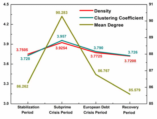
Figure 1.
Trend of statistical characteristics of global stock market networks.
Since then, these three indicators have shown a downward trend, and reached a lower peak during the European debt crisis. The subprime mortgage crisis severely damaged the European economy, and excessive expansionary fiscal policy eventually led to the outbreak of the debt crisis. After that, the downturn in the European stock markets caused a global stock market slump through three channels containing trade, finance, and investor expectations [41]. During the recovery period, the economic fundamentals of each country or region returned to stable.
It can be found that network structures are relatively stable during the non-crisis period and undergo drastic shocks under the impact of extreme events. The risk spillovers of the global stock markets reflect typical event-driven and time-varying characteristics.
3.2. Node Centrality and Flow Hierarchy of Connectedness Networks
Figure 2 represents the topological graphs of four periods, which show the evolution of node centrality in the four periods. For convenience, we use the abbreviation of each country to represent its corresponding stock index. As the directed and weighted network show, the higher the indegree, the greater the effects of risk absorption and the larger the node; on the contrary, the weighted outdegree represents the degree of risk spillover. Besides, the node indicated with the arrow is the country/region that sends risk, and the thicker and deeper the arrows, the greater the strength of the connection between the two nodes.
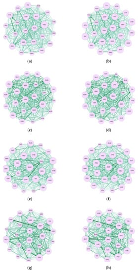
Figure 2.
Topological graphs of the four periods: (a) weighted outdegree in the stationary period; (b) weighted indegree in the stationary period; (c) weighted outdegree in the subprime crisis period; (d) weighted indegree in the subprime crisis period; (e) weighted outdegree in the European debt crisis period; (f) weighted indegree in the European debt crisis period; (g) weighted outdegree in the recovery period; (h) weighted indegree in the recovery period.
The topology structure proves that fluctuations can differently influence divergent stock markets in the same network, and some stock markets have the dynamic power to influence other nodes. For example, France is the largest node in Figure 2a, indicating that France is the center of Europe and has a greater risk spillover effect on other countries. Besides, the rank of central risk spillover/absorption nodes in the four periods are time varying.
The subprime crisis period is the peak of global systemic risk [48], when risk spillover or risk absorption of all countries/regions were significantly stronger than other periods. This finding is authenticated as the arrows between nodes had generally become deeper and thicker during this period. It is obvious that the outdegree of the USA had greatly increased, indicating that the US stock market had significantly improved its centrality of risk spillover network and caused a general shock to the world stock markets. France still exerted the strongest risk spillover, which was at the center of the risk spillover network; meanwhile Japan and Korea were more sensitive to crisis, having the greatest capability of risk absorption, and suffered severe economic crisis. Centrality of the connectedness networks revealed the transmission path of the crisis to a certain degree. The crisis effect overflowed from the US stock market (the origin point) towards the world. In Europe, it mainly affected the surroundings through FRA (bridge effects). In Asia, it was mainly absorbed by JAP and KOR before spreading outward.
During the European debt crisis, the debt crisis of peripheral countries like Greece quickly disseminated to the entire Eurozone [49]. Open developed countries/regions have a higher degree of risk spillover; for example, European leaders such as France and the UK soon became the center of the risk spillover network and greatly affected other markets. The outbreak of the crisis has greatly increased the interdependence between European stock markets. Countries in the Americas region were closely connected with countries in Europe, and the crisis was transmitted from central European countries to USA and CAN, which is consistent with the findings of BenMim and BenSaïda [50]. In Asia, HKG had the highest degree of openness, so it also became a major risk spillover node; whereas open developing countries suffered the highest external risks, as Thailand became the main risk transfer and bearing destination of developed countries.
The structure of global connectedness networks and the hub’s central position evolved with the disappearance of the crisis. From a horizontal comparison, there is a significant asymmetry in global risk spillover, and developed countries/regions are the main source of financial crisis. From a vertical comparison, the risk spillover effects of traditional developed countries (represented by USA) have weakened, whereas those of financial emerging economies (represented by China) are growing, lending support to the result of Zhang et al. [1]
Regarding the conformity of our results to the previous studies, the tightening composition and more centralized topology prove the proposition that risk spillover intensifies during crisis periods [1,18,51]. Concerning difference, the prominent risk senders and recipients found in our volatility spillover network are not the same as those identified in other studies. Liu et al. [15] find that for an average ranking, Korea and Brazil are the largest volatility sender and recipient, respectively, throughout the sampling periods; meanwhile, Mensi et al. [18] conclude that U.S. and GIPSI (except Spain and Greece markets) markets are net senders of shocks, and the rest of the stock markets are receivers. In our study, we identify that France is on average the largest volatility sender, and the UK is the largest risk receiver on average. The differences may be accounted for by the different data used (stock index and data interval), and the different results can be regarded as evidence of the event-driven and time-varying spillover effects.
In Figure 3, we use the chord diagram to visualize the distribution of risk contagion strength in four different periods so that the hierarchical structures of risk flows could be revealed. An arc is mapped to a country or region of the risk spillover networks and a chord is a link that connects two arcs together, whose width represents the strength of the interaction between the two connected nodes. The wider the chord, the stronger the interaction. In Figure 3, if one side of the chord is closer to the arc than the other side, then the arc corresponding to the closer side represents risk spillover.
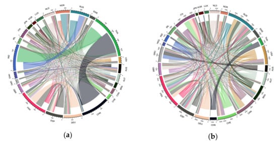
Figure 3.
Chord diagrams in four periods: (a) stationary period; (b) subprime crisis period; (c) European debt crisis period; (d) recovery period.
In Figure 3a, the chord that connects THA with CHN is the most prominent, followed by the chord between IND and THA. This means that during this period, the unidirectional spillover effect of the Thai stock market on the Chinese stock market was the strongest, followed by the impacts of IND on THA. Figure 3b shows that the widths of chords that had greater impacts in the last period decreased with the emergence of the subprime crisis. Moreover, chord strengths are more evenly distributed in Figure 3b than those in Figure 3a since more spillover links surged during the crisis time at the expense of waning prominent ties. This is indicative of the worldwide impacts of the subprime crisis. Figure 3c indicates that during the European debt crisis, the interaction within the European stock markets increased, and the node involvements captured by arc lengths of European countries are more evenly distributed. There are prominent risk linkages which shoulder a large part of the transmission quantities, and risk spillover occurs mainly from developed economies to emerging markets. For instance, USA and CAN have significant two-way spillover effects, whereas the one-way spillover impacts of CAN on THA, USA on THA, and HKG on CHN are more evident. Figure 3d shows that during the recovery period, the economic fundamentals of each country/region had stabilized, stock market volatilities had leveled off, and risk contagion effects tended to be evenly distributed again.
To sum up, the results of flow hierarchy analysis are generally in line with the findings of Liu et al. [15] in terms of the accumulative distribution of the weighted edges and the direction of key volatility transmission paths. The deviation of our study is that the intensities of the connections during the subprime crisis and the European debt crisis are more even on a global scale and on a European scale, respectively, indicating the differing radiation ranges of these two financial crises.
3.3. Factors Affecting the Weighted Connectedness Networks
GERGM is used to model and simulate the volatility spillover networks in the four periods. The estimation results are shown in Figure 4. In respect of the endogenous network structures, the parameters of mutual dyads and out two-stars are significantly positive in the four investigation periods, whereas the parameters of in two-stars are significantly negative, supporting Hypothesis 1 and partially supporting Hypothesis 2. This indicates that the volatility spillover network exhibits reciprocity among the stock markets of countries and regions and there exist giant risk diffusers in the market rather than concentrated risk absorbers. These results are consistent with the topological analysis in Section 3.2. in that risk contagion flows are bi-directional and countries like America and France are identified as the main risk originators. These results prove the finding of Luchtenberg and Vu [22] regarding the prevalence of bi-directional risk contagion. Notably, the effects of mutual dyads are observed to be stronger during non-crisis periods than in crisis periods, while the opposite trend is observed for the network configuration of out two-stars. The contrast indicates an increase in the proportion of giant risk emitters and a weakening of bi-directional relationships during crisis periods.
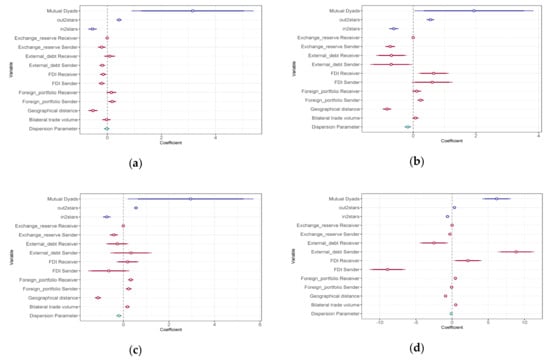
Figure 4.
Estimates of the parameters for covariates and dependence terms in the four periods: (a) stationary period; (b) subprime crisis period; (c) European debt crisis period; (d) recovery period.
Next, the impacts of nodal attributes and exogenous networks on network formation mechanism are analyzed to derive the following results.
- (1)
- Exchange reserve: The exchange reserve receiver has no significant effects since the parameter estimates are not significantly different from zero. However, parameters of exchange reserve senders remain negative consistently in the four periods, and the inhibitory effect of exchange reserve on risk spillover gets stronger as time goes by. Hypothesis 3 is partially supported. As the increased fluctuation in the foreign exchange markets is proved to induce higher volatility spillover in the stock market [10], sufficient exchange reserves can be regarded as a buffer stock to respond to fluctuations in international payments, ensuring that countries can calmly respond to sudden financial crisis and meet the demands for maintaining stable local currency exchange [32].
- (2)
- External debt: Both the external debt sender and receiver effects are negative in subprime crisis. This can be explained by the proposition of Ye and Han [52] that the easier countries having access to international funding during a crisis, the more they can suppress risk contagion. Although there was no statistical significance during the European debt crisis, impacts of external debt on risk contagion in the subsequent recovery period are quite clear, with the external debt receiver effect being negative and the sender effect being positive. One possible explanation is that the European debt crisis exerts a lag effect in the recovery period and both debtor and creditor countries are extremely vulnerable during the subsequent period. When debtor countries have difficulty repaying foreign debts on time, there will be difficult capital turnover occurring in creditor banks, causing credit crunches and payment crises in creditor countries. Hypothesis 4 is corroborated. It is worth noting that our result differs from Zhang et al. [1] who identified a consistently positive effect of government debt on systemic risk in the G20 stock markets network from 2006 to 2017. The difference may be mainly attributable to our model specification, which allows the examination of risk spillover and absorption channels respectively and consequently elicits more detailed findings.
- (3)
- Capital account: In terms of FDI, the parameters of FDI receivers in the subprime crisis and recovery periods are both positive, which can be explained by the “sudden flight” effect proposed by Warnock and Rothenberg [25]. After the crisis breaks out in one country, causing domestic credit contraction and liquidity insufficiency, domestic investors will withdraw their investment funds (such as FDI) from other countries to maintain domestic liquidity and avoid risks. This short-term outflow of large amounts of funds will cause turbulence in other countries’ financial markets, and finally result in global contagion. Therefore, markets of emerging countries that rely heavily on foreign direct investment are more likely to absorb external financial risks and suffer huge economic losses because of the “sudden flight” effect. Besides, one possible explanation of the positive parameter in recovery period is that the European debt crisis exerts a lag effect. The parameters of FDI senders during non-crisis periods are both negative, which may be related to the overall stability of the international economic environment. Under the premise of stable global economic conditions, the more foreign investments one country absorbs, the more stably its economy develops, and the weaker the possibility of risk spillover [53]. All results support Hypothesis 5. Unlike the studies of Zhang et al. [5], which identify a positive link between capital liquidity and systematic risk, our model differentiates between risk absorption and risk spillover while taking into account relational data and network endogeneity which could map the specific condition of FDI influence.In terms of FPI, whether significant or not, the parameters of foreign portfolio receiver and sender are all positive except in the recovery period, implying that FPI significantly amplifies both risk spillover and absorption. Thus, Hypothesis 6 is verified. These results lend support to the cross-market rebalancing theory proposed by Kodres and Pritsker [24]. The rationale is that the higher the FPI of the crisis origin country, the more losses the investor countries will suffer, and the more the investments will be diverted from other countries, such as neighboring or trade-linked countries, for the consideration of portfolio rebalancing [24]. This will consequently amplify the risk spillover of origin countries and risk absorption of closely related countries due to investment readjusting. Albeit different in methodology, our results are parallel to those of Schiavone [54] in the verification of portfolio rebalancing with real data. The additional contribution of our method lies in our disentangling of the FPI channel by phases and spillover ends (recipient or sender).
- (4)
- Geographic distance: The constantly negative parameters of geographical distance during the four periods prove the proposition that geographic proximity aggravates risk transmission. This is consistent with the “neighborhood effects” proposed by Haile and Pozo [40]. In particular, this effect is amplified during the crisis periods compared with the non-crisis periods. Hypothesis 7 is supported. Countries in the same region have similar political and economic conditions and are closely linked. The crisis outbreak of a particular country will drag other countries in the same region into the quagmire [41]. The geographic distances from the risk epicenter also determine the likelihood of contagion [55]. Our result is contrary to that of Zhang et al. [5], which does not identify a link between the geographical factor and risk spillover. The difference could be ascribed to the measurement difference of geographic matrix between spatial distance in ours and continent belonging in theirs.
- (5)
- International trade: The parameters of bilateral trade volumes are positive and significant since the European debt crisis period, indicating that trade links can promote the spread of shocks, which partially supports Hypothesis 8. It can be explained that with the deepening of the crisis, the crisis of financial markets is transmitted to the real economy [41], subsequently affecting trading partners and competitor countries through the income effect and price effect [42]. The positive effect of trade on risk contagion confirms the conclusion of Glick and Rose [47]. But it differs from the result of Zhang et al. [1], which indicates that trade has significantly negative effects on systemic risk. This result deviation could be traced to the different treatment of the trade variable. Trade, which is designated as a country attribute variable in the study of Zhang et al. [1], is treated as a relational matrix covariate in our study.
To sum up, risk contagion effects based on financial linkages are generally stronger than other exogenous-related contagions. The main channel for risk spillover is FPI, especially during the subprime crisis; the main channel for risk absorption is FDI, especially during the recovery period after the European debt crisis. Besides, due to a greater share in cross-border investments, the effect of FDI is stronger than FPI. After the risk spreads along the financial channels, the currency value of each country will be affected, which will subsequently affect the real economy and, in turn, exacerbate the spread of crisis through trade channels. In addition to these two channels, geographic proximity can exacerbate the spread of risk whenever and wherever. Maintaining a high level of exchange reserves and a moderate level of external debts can usually prevent the risk of large fluctuations in capital flows and smooth the fluctuation effects caused by capital shocks. Overall, the effects of risk contagion channels are superimposed on each other, and the intensity of each channel is evolved with the international economic context.
To assess goodness of fit for the estimated models, we compare the simulated networks’ structural attributes (whether they were included in the model simulations or not) with the observed networks. We evaluate how well our GERGM model fitted in nine different features. The in-degree (out-degree) distribution refers to the probability distribution of the in-degree (out-degree) of each node in the entire network. The goodness of fit diagnostics is shown in Figure 5.
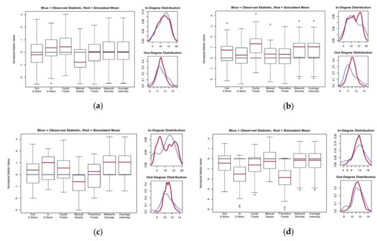
Figure 5.
Goodness of fit plots for the model fitted to the risk spillover networks: (a) stationary period; (b) subprime crisis period; (c) European debt crisis period; (d) recovery period.
Our model seems to converge as most of the observed values fall within the inter-quartile range of the GERGM simulation values [19]. Therefore, the simulated model is good at fitting with the observed network in the majority of the dependence features. Besides, trace plots of the simulated network density indicate that the model has converged (see Figure 6).
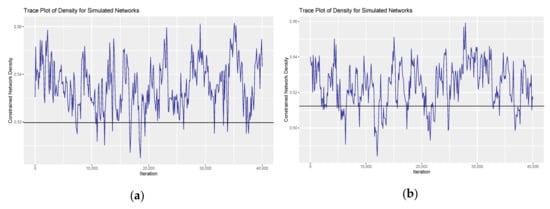
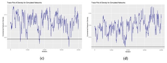
Figure 6.
Trace plot of network density for the simulated networks in the four periods: (a) stationary period; (b) subprime crisis period; (c) European debt crisis period; (d) recovery period.
In order to verify that our model is not degenerate, we processed the hysteresis analysis according to Snijders et al. [56] We simulated a large number of networks at values around the estimated parameter values, and plotted the average network density of each value to check the possibility for network density jumps due to small deviations in the parameter. Figure 7 shows the hysteresis plots for our model. The smooth upward tilted series of points exhibited in the graph of each period prove that the specification is not degraded.
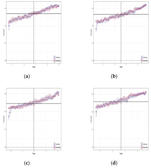
Figure 7.
Hysteresis plots for the simulated network in the four periods: (a) stationary period; (b) subprime crisis period; (c) European debt crisis period; (d) recovery period.
4. Conclusions
Considering the intrinsic nature of stock market connectedness, this paper establishes a holistic framework to study characteristics and influencing channels of volatility spillover across 24 major stock markets from 2004 to 2015. To this end, we apply generalized variance decomposition to estimate volatility spillover, based on which the weighted and directed networks are generated for the network evolution analysis in terms of the overall structure, node, and flow level. Following this, a recent development in network inference model, GERGM, is applied to reveal the channels for cross-market volatility linkages. Our model, which controls network endogeneity and addresses the relational attribute variables appropriately, sheds light on the topological dynamics and the evolving channels of connectedness networks in two aspects: a dynamic perspective juxtaposing crisis and non-crisis periods, and a contrasting perspective between risk absorption and risk spillover. This research enriches academic findings regarding risk contagion and brings benefits to policy-relevant practitioners.
4.1. Main Findings
The main findings of our research explain three issues concerning connectedness networks. One is the time-varying characteristics, the other two are concerned with the endogenous and exogenous formation mechanisms.
First, the network structure mutates during crisis periods, manifesting in the increased network density and tie strength. Additionally, the subprime crisis exerts stronger impacts than the European debt crisis. The developed markets are more influential and less sensitive to external shocks than emerging markets, thus the strength of risk transmitted from developed economies to emerging markets is generally greater than the reverse linkages. These results are in line with the findings of previous studies [1,18,44,51]. In addition, we identify France as, on average, the largest volatility sender, and the UK as the largest risk receiver on average, which corroborates Yarovaya et al. [57] on the role of the UK but differs from Yarovaya et al. [57] and Liu et al. [15] on the risk sender. Yarovaya et al. [57] and Liu et al. [15] reported that the most influential markets are the UK and Korea. France, as the largest volatility sender, was first identified in this research, justifying the potential of France as a benchmark of market volatility for investors.
Second, the simulated connectedness networks present reciprocity and preferential attachment characteristics. Specifically, we use GERGM to simulate the formation mechanisms of risk contagion. We find that both bilateral linkages between two stock markets and nodes’ preference in connecting to nodes with a higher risk outdegree promote risk contagion. The larger effect of out two-stars during crisis periods means that the proportion of giant risk emitters prominently increases, underscoring the risk sender’s role in amplifying risk contagion. This result lends support to the proposition that volatility spillovers exhibit evident multiple superposition phenomena [1], authenticating the paramount significance in monitoring both the hub node exerting direct effect and the structurally bridging nodes that act as the risk contagion intermediary.
Third, financial account linkages are the most prominent channel of volatility spillover. From the comparison of the four periods, the main channel for risk spillover is FPI, especially during the subprime crisis; and the main channel for risk absorption is FDI, especially during the post-crisis recovery period. This result is in contrast with the existing literature, most of which shows that either FDI or FPI is positively related to risk spillover or systemic correlation without considering risk absorption [5,54]. Our study distinguishes the impacts between risk absorption and risk spillover from a dynamic perspective, thus drawing more detailed conclusions. The above results lend support to the proposition that the collapse of financial markets is mainly transmitted to macro fundamentals through capital flows, which later leads to risk contagion worldwide [58]. Therefore, while actively engaged in investment and financing activities, more attention should be paid to diversifying investments and keeping adequate foreign exchange reserves to deal with sudden capital flights. Moreover, trade links and geographical proximity amplify risk contagion. The result is contrary to that of Zhang et al. [1,5]. Different treatment of trade variables and the different criteria of the geographical adjacency matrix may explain the inconsistent results. This contrast indicates that divergence exists in the estimation of spillover channels between econometric models and network inference models, which should be considered with caution in future studies. Last but not least, a high level of exchange reserves and a moderate level of external debts strengthen a country’s robustness to risks.
4.2. Policy Implications
From a practical point of view, this study is of certain value for risk regulators.
First, there are implications for improving risk early warning system. It is necessary to establish a daily monitoring mechanism for international transmission of financial risks and achieve two-way management manifesting in the full use of advantages and prudent prevention and control of risks. Countries should also establish comprehensive evaluation index systems with fast updating data and high transparency, covering various markets (industries).
Second, with regards to improving management of risk contagion channels: when the financial crisis occurs in a country, other countries should cut off trade and financial links with that country in time to prevent risk contagion. The governments of the recipient country of foreign investment should inject capital or provide loans to banks and enterprises in time to maintain sufficient and stable liquidity in the financial market. The governments of emerging countries should consciously weaken the degree of trade and financial dependence on developed countries. In addition, countries should strictly control the scale of debt issuance, adjust foreign debt holdings, and handle relationships with major international centers to make it easier to obtain international loan assistance in times of crisis.
Third, there are implications for the strengthening of international cooperation among financial regulators around the world. In the context of economic globalization, the global stock markets can be regarded as a complex economic ecosystem embedded in symbiotic relationships, so it is necessary to strengthen the international sharing of management information concerning financial risk contagion. Especially in regions with obvious geographical clustering, cooperation should be strengthened prominently. In addition, the prevention of international financial risk contagion is a long-term process. Therefore, it is of great importance to establish a long-term risk governance system in combination with global forces, along the whole process of risk early warning, management, and recovery.
Author Contributions
Conceptualization, D.M.; methodology, D.M. and R.C.; software, D.M. and R.C.; formal analysis, Y.Z. and D.M.; investigation, Y.Z.; writing—original draft preparation, Y.Z. and R.C.; writing—review and editing, D.M. and Y.Z.; funding acquisition, D.M. All authors have read and agreed to the published version of the manuscript.
Funding
This research was funded by the National Natural Science Foundation of China (grant number 71774128), Fundamental Research Funds for the Central Universities of China (grant number 2019VI059), and the National Natural Science Foundation of China (grant number 19BJY057).
Conflicts of Interest
The authors declare no conflict of interest.
References
- Zhang, W.; Zhuang, X.; Lu, Y. Spatial spillover effects and risk contagion around G20 stock markets based on volatility network. N. Am. J. Econ. Financ. 2020, 51, 101064. [Google Scholar] [CrossRef]
- Deev, O.; Lyócsa, Š. Connectedness of financial institutions in Europe: A network approach across quantiles. Physica A 2020, 550, 124035. [Google Scholar] [CrossRef]
- Fan, X.; Wang, Y.; Wang, D. Network connectedness and China’s systemic financial risk contagion—An analysis based on big data. Available online: https://www.sciencedirect.com/science/article/pii/S0927538×19305256 (accessed on 24 March 2020).
- Kang, S.H.; Lee, J.W. The network connectedness of volatility spillovers across global futures markets. Physica A 2019, 526, 120756. [Google Scholar] [CrossRef]
- Zhang, W.; Zhuang, X.; Lu, Y.; Wang, J. Spatial linkage of volatility spillovers and its explanation across G20 stock markets: A network framework. Available online: https://www.sciencedirect.com/science/article/pii/S1057521919305381 (accessed on 21 January 2020).
- Wang, G.-J.; Jiang, Z.-Q.; Lin, M.; Xie, C.; Stanley, H.E. Interconnectedness and systemic risk of China’s financial institutions. Emerg. Mark. Rev. 2018, 35, 1–18. [Google Scholar] [CrossRef]
- Yu, J.-W.; Xie, W.-J.; Jiang, Z.-Q. Early warning model based on correlated networks in global crude oil markets. Physica A 2018, 490, 1335–1343. [Google Scholar] [CrossRef]
- Wang, G.J.; Xie, C.; He, K.; Stanley, H.E. Extreme risk spillover network: application to financial institutions. Quant. Financ. 2017, 17, 1–23. [Google Scholar] [CrossRef]
- Lyócsa, Š.; Výrost, T.; Baumöhl, E. Return spillovers around the globe: A network approach. Econ. Model. 2019, 77, 133–146. [Google Scholar] [CrossRef]
- Baumöhl, E.; Kočenda, E.; Lyócsa, Š.; Výrost, T. Networks of volatility spillovers among stock markets. Physica A 2018, 490, 1555–1574. [Google Scholar] [CrossRef]
- Peralta, G.; Zareei, A. A network approach to portfolio selection. J. Empir. Financ. 2016, 38, 157–180. [Google Scholar] [CrossRef]
- Výrost, T.; Lyócsa, Š.; Baumöhl, E. Network-based asset allocation strategies. N. Am. J. Econ. Financ. 2019, 47, 516–536. [Google Scholar] [CrossRef]
- Billio, M.; Getmansky, M.; Lo, A.W.; Pelizzon, L. Econometric measures of connectedness and systemic risk in the finance and insurance sectors. J. Financ. Econ. 2012, 104, 535–559. [Google Scholar] [CrossRef]
- Diebold, F.X.; Yılmaz, K. On the network topology of variance decompositions: Measuring the connectedness of financial firms. J. Econom. 2014, 182, 119–134. [Google Scholar] [CrossRef]
- Liu, X.; An, H.; Li, H.; Chen, Z.; Feng, S.; Wen, S. Features of spillover networks in international financial markets: Evidence from the G20 countries. Physica A 2017, 479, 265–278. [Google Scholar] [CrossRef]
- Hautsch, N.; Schaumburg, J.; Schienle, M. Financial Network Systemic Risk Contributions*. Rev. Financ. 2014, 19, 685–738. [Google Scholar] [CrossRef]
- Papana, A.; Kyrtsou, C.; Kugiumtzis, D.; Diks, C. Financial networks based on Granger causality: A case study. Physica A 2017, 482, 65–73. [Google Scholar] [CrossRef]
- Mensi, W.; Boubaker, F.Z.; Al-Yahyaee, K.H.; Kang, S.H. Dynamic volatility spillovers and connectedness between global, regional, and GIPSI stock markets. Financ. Res. Lett. 2018, 25, 230–238. [Google Scholar] [CrossRef]
- Diebold, F.X.; Yilmaz, K. Trans-Atlantic Equity Volatility Connectedness: US and European Financial Institutions, 2004–2014. J. Financ. Econ. 2016, 14, 81–127. [Google Scholar] [CrossRef]
- Fernández-Rodríguez, F.; Gómez-Puig, M.; Sosvilla-Rivero, S. Using connectedness analysis to assess financial stress transmission in EMU sovereign bond market volatility. J. Int. Financ. Mark. Inst. Money 2016, 43, 126–145. [Google Scholar] [CrossRef]
- Hwang, E.; Min, H.-G.; Kim, B.-H.; Kim, H. Determinants of stock market comovements among US and emerging economies during the US financial crisis. Econ. Model. 2013, 35, 338–348. [Google Scholar] [CrossRef]
- Luchtenberg, K.F.; Vu, Q.V. The 2008 financial crisis: Stock market contagion and its determinants. Res. Int. Bus. Financ. 2015, 33, 178–203. [Google Scholar] [CrossRef]
- Mobarek, A.; Muradoglu, G.; Mollah, S.; Hou, A.J. Determinants of time varying co-movements among international stock markets during crisis and non-crisis periods. J. Financ. Stab. 2016, 24, 1–11. [Google Scholar] [CrossRef]
- Kodres, L.; Pritsker, M. A Rational Expectation Model of Financial Contagion. J. Financ. 2002, 57, 769–799. [Google Scholar] [CrossRef]
- Warnock, F.; Rothenberg, A. Sudden Flight and True Sudden Stops. Rev. Int. Econ. 2011, 19, 509–524. [Google Scholar] [CrossRef][Green Version]
- Samitas, A.; Tsakalos, I. How can a small country affect the European economy? The Greek contagion phenomenon. J. Int. Financ. Mark. Inst. Money 2013, 25, 18–32. [Google Scholar] [CrossRef]
- Kenourgios, D. On financial contagion and implied market volatility. Int. Rev. Financ. Anal. 2014, 34, 21–30. [Google Scholar] [CrossRef]
- Mollah, S.; Quoreshi, A.M.M.S.; Zafirov, G. Equity market contagion during global financial and Eurozone crises: Evidence from a dynamic correlation analysis. J. Int. Financ. Mark. Inst. Money 2016, 41, 151–167. [Google Scholar] [CrossRef]
- Diebold, F.; Yilmaz, K. Measuring Financial Asset Return and Volatility Spillovers, With Application to Global Equity Markets. Econ. J. 2009, 119, 158–171. [Google Scholar] [CrossRef]
- Wilson, J.D.; Denny, M.J.; Bhamidi, S.; Cranmer, S.J.; Desmarais, B.A. Stochastic weighted graphs: Flexible model specification and simulation. Soc. Netw. 2016, 49, 37–47. [Google Scholar] [CrossRef]
- Dimitriou, D.; Kenourgios, D.; Simos, T. Global financial crisis and emerging stock market contagion: A multivariate FIAPARCH–DCC approach. Int. Rev. Financ. Anal. 2013, 30, 46–56. [Google Scholar] [CrossRef]
- Caballero, R.; Panageas, S. A Quantitative Model of Sudden Stops and External Liquidity Management. Available online: https://ssrn.com/abstract=703241 (accessed on 12 April 2005).
- Jayaraman, T.K.; Lau, E. Does external debt lead to economic growth in Pacific island countries. J. Policy Model. 2009, 31, 272–288. [Google Scholar] [CrossRef]
- Gómez-Puig, M.; Sosvilla-Rivero, S. Causes and hazards of the euro area sovereign debt crisis: Pure and fundamentals-based contagion. Econ. Model. 2016, 56, 133–147. [Google Scholar] [CrossRef]
- Edo, S.; Osadolor, N.E.; Dading, I.F. Growing external debt and declining export: The concurrent impediments in economic growth of Sub-Saharan African countries. Int. Econ. 2020, 161, 173–187. [Google Scholar] [CrossRef]
- Peek, J.; Rosengren, E.S. The International Transmission of Financial Shocks: The Case of Japan. Am. Econ. Rev. 1997, 87, 495–505. [Google Scholar] [CrossRef]
- Longstaff, F.A. The subprime credit crisis and contagion in financial markets. J. Financ. Econ. 2010, 97, 436–450. [Google Scholar] [CrossRef]
- Yuan, K. Asymmetric Price Movements and Borrowing Constraints: A Rational Expectations Equilibrium Model of Crises, Contagion, and Confusion. J. Financ. 2005, 60, 379–411. [Google Scholar] [CrossRef]
- Markowitz, H. Portfolio Selection. J. Financ. 1952, 7, 77–91. [Google Scholar] [CrossRef]
- Haile, F.; Pozo, S. Currency crisis contagion and the identification of transmission channels. Int. Rev. Econ. Financ. 2008, 17, 572–588. [Google Scholar] [CrossRef]
- Gorea, D.; Radev, D. The euro area sovereign debt crisis: Can contagion spread from the periphery to the core? Int. Rev. Econ. Financ. 2014, 30, 78–100. [Google Scholar] [CrossRef]
- Gerlach, S.; Smets, F. Contagious speculative attacks. Eur. J. Polit. Econ. 1995, 11, 45–63. [Google Scholar] [CrossRef]
- Filardo, A.; George, J.; Loretan, M.; Ma, G.; Munro, A.; Shim, I.; Wooldridge, P.; Yetman, J.; Zhu, H. The international financial crisis: timeline, impact and policy responses in Asia and the Pacific. Available online: https://www.bis.org/repofficepubl/arpresearch200908.2.htm (accessed on 9 August 2009).
- Gong, C.; Tang, P.; Wang, Y. Measuring the network connectedness of global stock markets. Physica A 2019, 535, 122351. [Google Scholar] [CrossRef]
- Owusu Junior, P.; Alagidede, I. Risks in emerging markets equities: Time-varying versus spatial risk analysis. Physica A 2020, 542, 123474. [Google Scholar] [CrossRef]
- Calvo, G.A.; Mendoza, E.G. Rational contagion and the globalization of securities markets. J. Int. Econ. 2000, 51, 79–113. [Google Scholar] [CrossRef]
- Glick, R.; Rose, A.K. Contagion and trade: Why are currency crises regional? J. Int. Money Financ. 1999, 18, 603–617. [Google Scholar] [CrossRef]
- Boubaker, S.; Jouini, J.; Lahiani, A. Financial contagion between the US and selected developed and emerging countries: The case of the subprime crisis. Q. Rev. Econ. Financ. 2016, 61, 14–28. [Google Scholar] [CrossRef]
- Bhanot, K.; Burns, N.; Hunter, D.; Williams, M. News spillovers from the Greek debt crisis: Impact on the Eurozone financial sector. J. Bank Financ. 2014, 38, 51–63. [Google Scholar] [CrossRef]
- BenMim, I.; BenSaïda, A. Financial contagion across major stock markets: A study during crisis episodes. N. Am. J. Econ. Financ. 2019, 48, 187–201. [Google Scholar] [CrossRef]
- Su, X. Measuring extreme risk spillovers across international stock markets: A quantile variance decomposition analysis. N. Am. J. Econ. Financ. 2020, 51, 101098. [Google Scholar] [CrossRef]
- Ye, Q.; Han, L.-Y. Contagion channels and mechanisms of the subprime mortgage crisis in global financial markets. Xitong Gongcheng Lilun yu Shijian/Syst. Eng. Theory Pract. 2014, 34, 2483–2494. [Google Scholar] [CrossRef]
- Hansen, H.; Rand, J. On the Causal Links Between FDI and Growth in Developing Countries. World Econ. 2006, 29, 21–41. [Google Scholar] [CrossRef]
- Schiavone, A. Estimating the contagion effect through the portfolio channel using a network approach. Available online: https://ssrn.com/abstract=3165421 (accessed on 28 March 2018).
- Kelejian, H.H.; Tavlas, G.S.; Hondroyiannis, G. A Spatial Modelling Approach to Contagion Among Emerging Economies. Open Econ. Rev. 2006, 17, 423–441. [Google Scholar] [CrossRef]
- Snijders, T.; Pattison, P.; Robins, G.; Handcock, M. New Specifications for Exponential Random Graph Models. Sociol. Methodol. 2006, 36, 99–153. [Google Scholar] [CrossRef]
- Yarovaya, L.; Brzeszczyński, J.; Lau, C.K.M. Intra- and inter-regional return and volatility spillovers across emerging and developed markets: Evidence from stock indices and stock index futures. Int. Rev. Financ. Anal. 2016, 43, 96–114. [Google Scholar] [CrossRef]
- Masson, P. Contagion: macroeconomic models with multiple equilibria. J. Int. Money Financ. 1999, 18, 587–602. [Google Scholar] [CrossRef]


© 2020 by the authors. Licensee MDPI, Basel, Switzerland. This article is an open access article distributed under the terms and conditions of the Creative Commons Attribution (CC BY) license (http://creativecommons.org/licenses/by/4.0/).