Abstract
Passenger behavior analysis is a key issue in passenger assignment research, in which the path choice is a fundamental component. A highly complex transit network offers multiple paths for each origin–destination (OD) pair and thus resulting in more flexible choices for each passenger. To reflect a passenger’s flexible choice for the transit network, the optimal strategy was proposed by other researchers to determine passenger choice behavior. However, only strategy links have been searched in the optimal strategy algorithm and these links cannot complete the whole path. To determine the paths for each OD pair, this study proposes the depth-first path generation algorithm, in which a strategy node concept is newly defined. The proposed algorithm was applied to the Beijing metro network. The results show that, in comparison to the shortest path and the K-shortest path analysis, the proposed depth-first optimal strategy path generation algorithm better represents the passenger behavior more reliably and flexibly.
1. Introduction
Passenger behavior analysis is a fundamental issue for urban rail transit research, where the path choice or route choice is the dominant aspect. The shortest path scheme is the most popular solution for path choice analysis. To find the shortest path, several researchers have made a great contribution. The Dijkstra shortest path algorithm is the benchmark in this topic where the link travel time is fixed. In 1984, the Dijkstra algorithm was successfully applied to the frequency-based transit network [1]. Since then, this algorithm has been studied extensively in the fields of computer science, communication engineering and transportation engineering. Although the Dijkstra algorithm has the ability to find the shortest path in un-circled transportation networks, it can be interpreted as breadth-first searching and a lot of “unnecessary” steps might be carried out before reaching the destination node [2]. To accelerate the search, Bander [3] proposed a new heuristic searching algorithm that is termed Interruptible A (IA) to accelerate the search by introducing the island-stops concept. An adaptation of the A* algorithm was proposed [4], which developed improved lower bounds on the minimum travel times to solve the instances of the one-to-one dynamic fastest path problem. Compared with the Dijkstra algorithm, the Dial algorithm does not enumerate all the feasible paths, which accelerates the solving efficiency [5]. However, because of the strict path definition, the Dial algorithm can find the paths in the figure where there is a ring route in it. Following the phenomenon that a passenger cares only about a part of the network before the path determination, Zhou [6] redefined the passenger path based on the transfer station to overcome the shortcoming of the Dial algorithm. Thus, the ring route path searching problem for the Dial algorithm was easily solved.
Note that these algorithms are designed based on the link travel time. However, passenger behavior is also impacted by path transfer times and comfort level. For instance, one may prefer to choose the shortest path, while others prefer to choose a feasible detour-path due to the availability of transport seats. To find other feasible paths in the network, K-shortest path algorithms are proposed to search for more paths rather than the shortest path. Hershberger et al. [7] proposed a replacement paths algorithm, which optimistically used a fast subroutine, and then it switches to a slower but correct algorithm if the subroutine is known to fail. Nevertheless, the problem of high-complexity for the path searching algorithm still needs to be solved, especially for a complex road network. Several researchers have tried to improve the searching algorithm efficiency to support the online passenger assignment simulation, which takes real-time automatic fare collection (AFC) data as the input and obtains the real-time loading factor for each train. Depth-first searching is discussed in the path searching algorithm [8]. Xu et al. [9] proposed a depth-first deleting link algorithm, which deleted one link in the shortest path and found the replaced path. Liu [10] and Liu [11] combined the depth-first algorithm with a branch-and-bound algorithm to decrease the algorithm complexity. Besides the depth-first searching algorithm, some heuristic algorithms, such as the Genetic Algorithm [12,13] and the Simulated Annealing algorithm [14,15], are also designed to find the K-shortest path. To improve the solving efficiency, some combined heuristic algorithms have been studied, such as the Immune Genetic Algorithm [16,17] and Particle Swarm-Ant Colony Optimization [18].
All of the above methods are widely used in a road network. Finding the K-shortest paths in the transit network is different from that in a road network. This is because, in comparison to the road network, the transit network is a combination of network line topology and train schedules, which contains temporal and spatial constraints, while the line topology is only focused on the spatial constraints. There are some research working on the algorithmic complexity of spatial arrangements. Papadimitriou evaluated the algorithmic complexity of landscapes with Kolmogorov complexity [19] and ultrametric distances [20]. Derrible and Kennedy [21] applied network science methodologies within 33 metro systems in the world and offered application to the robustness of metros. As a result, finding the K-shortest path in the schedule-based network (SBN) is much more difficult in comparison to the static physics network [22]. Inspired by Tong and Richardson (1984), Huang [23] and Friedrich et al. [24] researched path searching in SBN. Niu et al. [25] found that classical algorithms could not obtain the results efficiently in the SBN. Some new searching algorithms such as the Fibonacci heap method from computer science [26] and space-time prisms [27] are proposed to find the K-shortest path in SBN.
Although the K-shortest path can illustrate passenger behavior in the transit network, there are some shortcomings for passenger analysis. First, not all of the paths from the K-shortest path results are feasible paths for passengers. When compared to the shortest path, other path results may have more transfers and a longer path travel time. Generally, if the travel time of a certain path exceeds the tolerance index, which represents the extra travel time compared with the shortest path, this path is considered to be invalid and should be deleted [28]. However, the setting of the tolerance index is normally based on experience. Second, it is hard to determine the value of K in the K-shortest path. K could be three or five, which is also an empirical setting. Finally, it is assumed that in the K-shortest path assignment, the passengers would not change their paths until they reach their destinations. This is not suitable to describe the passenger’s flexible path choice behavior.
To overcome the above shortcomings, in 1989, the “optimal strategy” was proposed by Spiess and Florian [29]. It was first applied to a common bus network to determine which bus service could be selected in the common bus route. Whether at the trip origin or the stops along the trip, the passenger would select the first bus service from the optimal strategy set. In this way, a passenger’s path could not be determined at the beginning since he/she could choose during the journey. Compared with the K-shortest path and the shortest path assignment, with the optimal strategy, the description of the passenger path choice behavior is more practical [30].
The optimal strategy can describe the passenger behavior but their paths are not determined until they finish their trip because the optimal strategy set only contains the optimal links for each origin–destination (OD) pair. To analyze the passenger path from the optimal strategy, this study proposes a new concept called “the strategy node”. Based on the strategy node, a depth-first optimal strategy path generation algorithm is proposed, which was applied to the Beijing metro network to identify passenger behavior.
This paper is organized as follows. In Section 2, the optimal strategy is presented to express the calculation for the optimal strategy. In Section 3, the depth-first-based optimal strategy path generation algorithm is described in detail to generate the path from the optimal strategy and the difference between the optimal strategy path and the shortest path is analyzed. The proposed algorithm was verified to be superior to the shortest path algorithm within the Beijing metro network. Finally, the discussion, conclusions and directions for our future work are presented in the last two section.
2. Optimal Strategy Model and Algorithm
2.1. Symbols and Terminology
The service network can be represented as G = {E, I, L}, where I is the node in the network, including the physical node and the expanded dummy node such as the waiting node and the alighting node. E is the link set, which includes ingress and egress links, the waiting link and the in-vehicle link. L is the service set, which includes the different transit loops and stopping plans.
is the travel time for the link (a, b), which could be the in-vehicle time or the waiting time at the platform.
is the serve frequency for the link (a, b). For the in-vehicle link, it could be the train service frequency.
is the average waiting time for the link (a, b), which relates to .
represents the links start from node a.
indicates the links that end up with node a.
is the one trip strategy.
is the optimal strategy, which has the minimum expected travel time.
is the link from the optimal strategy, which starts with node a.
is the average waiting time at node a for .
is the service probability for the link (a, b) from the optimal strategy .
D is the destination set and d is the destination station.
v represents the passenger volume, where is the passenger volume at station a and is the passenger volume at the link (a, b).
is the entry passenger at node a.
is the expected travel time from a to the destination.
is the accumulated serve frequency at node a.
is the binary variable that determines if the link (a, b) belongs to the optimal strategy or not.
is the passenger total waiting time at node a.
2.2. Model and Algorithm
It is a common phenomenon that the passenger wants to complete their trip with the shortest travel time. The passenger choice model can be formulated as follows.
The object is to minimize the total travel time for all of the passengers in the network. The links which are satisfied with the model are contained in the optimal strategy set . Equation (2) is the passenger volume that is assigned to the link (a, b). Equation (3) is the flow conservation at node a. Equation (5) is the non-negative constraint for the passenger flow. This is a non-linear mixed-integer model. Equation (4) is the only non-linear constraint. Following the characteristic of the binary variable, Equation (4) can be relaxed as To simplify the model description, the variable , is introduced to represent the passenger total waiting time. The optimization model can be re-written as follows.
The new model is a mixed-integer model. To solve this model and find the optimal link for the optimal strategy, Spiess and Florian [28] already proposed the optimal strategy searching algorithm to find the best solution for the above model. The search algorithm is illustrated in Figure 1.
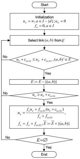
Figure 1.
Solution for the optimal strategy model.
The optimal strategy algorithm is similar to the backward labeling searching algorithm. The algorithm only determines the links that are used by the passengers to shorten their travel time. However, the path information is not included in the proposed algorithm. To overcome this problem, the depth-first path generation algorithm is proposed in the next section to generate a passenger path from the optimal strategy set.
3. Depth-First Optimal Strategy Path Generation Algorithm
3.1. Optimal Strategy Tree
The algorithm from Section 2 can determine the optimal strategy for each OD pair. Figure 2a presents the transit service map, which includes four kinds of service lines. The red and blue lines are the stop–stop transit services for two lines. The green line and the yellow line are the skip–stop transit services on the map. After applying the optimal strategy algorithm, the optimal strategy links are the remaining links as shown in Figure 2b.
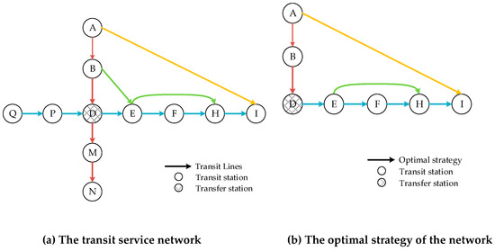
Figure 2.
Optimal strategy and the network.
The optimal strategy can be considered as the combination of the alternative links for each node. In Figure 3, the optimal strategy can be written as (A, B), (A, I), (B, D), (D, E), (E, F) (E, H), (F, H) and (H, I). If we take the link node as the decision tree node, then the link is the tree branch. The optimal strategy tree is shown in Figure 3.
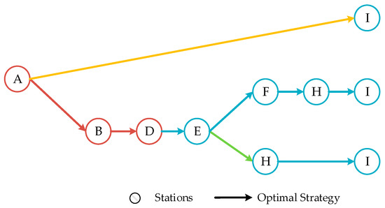
Figure 3.
Optimal strategy tree.
When passenger travel behavior is based on the optimal strategy, they will receive the first arrived services from the optimal strategy. The passenger behavior searches along the optimal tree. The complexity of the optimal tree is determined by the number of nodes and the alternative links that are connected with the node. In this way, the passenger’s choice can be taken as the path generated from the optimal strategy tree.
3.2. Strategy Node
There are two kinds of nodes in the optimal strategy tree. Some of the nodes are connected with only one link, such as Node B and Node D in Figure 3. For some of the nodes such as Node A and Node E, there is more than one connecting link. This means that the passengers could make their choice at these nodes according to the train arriving time or the link service frequency. This also follows the assumptions that were described by Spiess and Florian in 1989 [26]. To better distinguish these multi-link nodes, we refer to these nodes as the strategy node.
The strategy node is similar to the transfer station in the transit network, in which there is more than one attractive line. Although it is different from the physical transfer node, the strategy node can be in a real transfer station or a normal station that has multiple transit services. The number of optimal strategy paths is highly dependent on the number of strategy nodes for the given OD pair. Based on the characteristic of the strategy node, a depth-first path generation algorithm is proposed.
3.3. Depth-first Based Optimal Strategy Path Generation Algorithm
There are two kinds of searching algorithms: breadth-first searching and depth-first searching. Breadth-first searching is an algorithm that can start at any one node of the graph. The search does not go to the next depth level until all of the neighbor nodes at the present depth have been searched and the visited nodes are recorded in the stack.
The depth-first algorithm is different, which first explores the highest-depth nodes before being forced to backtrack and expand the shallower nodes [31]. In the depth-first searching algorithm, only one node needs to be saved in the stack for each depth level. This reduces a lot of saving work compared with the breadth-first searching algorithm, especially in a high depth level graph.
Usually, passengers will pass a lot of stations or stops when they finally reach their respective destinations. Because of the limited kinds of transit services in the network, the number of strategy nodes is significantly smaller in comparison to the total nodes in the network. Considering the strategy node characteristics, the depth-first based path generation algorithm was proposed, as shown in Figure 4. There are several terms in the algorithm, which are given below. All the abbreviations are listed in the Appendix A.
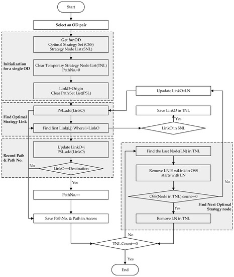
Figure 4.
Depth-first path generation algorithm.
Optimal strategy set (OSS). This refers to the definition by Spiess and Florian. For each OD pair, the selected optimal strategy links are recorded in this set and are ordered by the OD pair.
Optimal strategy node-list (SNL). For each OD pair, all of the optimal strategy nodes from the optimal strategy set are saved in this set.
Temporary optimal strategy node-list (TNL). When a strategy node is visited during the searching process, it is recorded in this set. This set saves and records the temporary strategy node.
Path-set list (PSL). The visited nodes are saved in this set by a sequence, which generates a path.
Path number set. This save the temporary path number.
The searching algorithm can be divided into four parts. The first part is the initialization section, which resets all of the sets that have been discussed for a specific OD pair. The second process is to find the optimal strategy link for the given link start node. The path and path number along the searching process are recorded in third part. Finally, if the visited node contains the optimal strategy node, the process will find the next optimal strategy part. The depth-first path generation algorithm is illustrated in Figure 4. These four parts are utilized in seven steps.
- Step 1:
- Initialize the optimal strategy set (OSS) and strategy node list (SNL) for each destination station. The OSS is the exact algorithm given in Figure 1. The temporal strategy node list (TNL) and the path-set are null. The path number is 0. The previous node (LinkO) is the origin from the OD pair.
- Step 2:
- Select the first link that started from the previous node from the OSS. Update the LinkO as the end of the selected link. Save the previous node in the path-set.
- Step 3:
- If the SNL contains the LinkO, add it to the TNL.
- Step 4:
- If the LinkO is the trip destination from the OD pair, go to Step 2. Otherwise, go to Step 5.
- Step 5:
- The path number adds one. Print out the path number and the elements from the path-set.
- Step 6:
- If the TNL is null, the algorithm stops. Otherwise, go to Step 7.
- Step 7:
- Select the last added node (LN) from the TNL. Remove the first optimal strategy link started with LN from OSS. If there is more than one link, start from LN from the updated OSS. Update LinkO as LN and go to Step 2. Otherwise, remove the LN in TNL and go to Step 6.
Consider Figure 3 as a toy model to demonstrate the algorithm in detail. From the definition of the strategy node, the SNL is {A, E}. During the first recursion, the path {A, B, D, E, F, H, I} can be determined. The nodes A, E are added to the TNL. Node E is the last added node (LN) in the TNL and the first optimal link for node E is (E, F). During the second recursion, link (E, F) is deleted from the OSS. The first optimal link for node E is (E, G). The second path {A, B, D, E, G, H, I} is generated. During the third recursion, after removing the link (E, G), there is no link left in OSS for node E. The node E is removed from the TNL. Link (A, B) for node A is deleted in the OSS. The path {A, I} was found. After removing the link (A, I) from the OSS, node A will be deleted from TNL. Up to now, there is no element in TNL, the searching process stops and all three paths from A to I are found.
The optimal strategy aims to minimize passenger travel time. The link will be added to the strategy if it has the potential to reduce the total travel time while considering the link travel time and the link waiting time. When generating the path with the optimal strategy links, it also contains the path that can save passengers’ total travel time. From this, the optimal strategy path and shortest path have something in common. If there is only one path generated in the optimal strategy, the path is the same as the shortest path. When there is more than one path in the optimal strategy, this means that there is more than the shortest path for the passengers when using the optimal strategy. There is no need to use the threshold to filter the path like the K-shortest path. This makes the path more feasible and workable.
4. The Application for the Beijing Metro Network
The Beijing metro network is a very busy transit system, and it serves more than 10 million passengers every day. During the morning peak hour, the minimal headway is about 90 s. Because of the high service frequency and the single service for a specific transit line, passengers do not care much about the timetable, and they would take the first coming train. This phenomenon is a similar behavior assumption in the optimal strategy model.
Meanwhile, the Beijing metro transit network is a very complex system that includes 17 lines, 344 stations and up to 574 km of transit lines by the end of 2017. In such a complex system, it is hard to determine if there should be three or five paths for each OD pair. A different OD pair may have a different number of feasible paths. After considering these, we used the optimal strategy and the proposed path generation algorithm to analyze the paths that were used by the passengers in the morning peak hour in Beijing.
4.1. The Topology of the Service Network
To represent the whole travel process in the network, the topology network of the Beijing metro was established. Take a part of Line 1 (blue) and Line 2 (red) as an example. In the partial network, there are five stations, Stations A–E, with one transfer Station B. As demonstrated in Figure 5, some dummy nodes that represent the platform and ticket gate are mapped to better illustrate the passenger’s precise boarding, alighting, waiting and walking behavior.
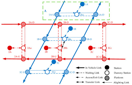
Figure 5.
Partial topology network of the Beijing metro.
Take Line 1, Station A as an example. For one station, there are three kinds of nodes. Node 1A is the ticket gate where the passengers enter the station. Node 1Aa is a platform dummy node to split the direction for the upstream and downstream. 1A-U and 1A-D are the upstream platform and downstream platforms, respectively. The links connected with the different nodes are access links, waiting links, alighting links and in-vehicle links.
For a transfer station, one thing should be clarified in advance. In Beijing, the transfer station is a combination of several individual stations that are connected with transfer tunnels. The platforms and entrances/exits are not shared. Take Figure 5 as an example. If a passenger enters Station 1B and wants to take Line 2, he or she should go to the transfer tunnel and go to Station 2B. From this, there is a transfer link that is connected to the dummy Nodes 1Bb and 2Bb.
4.2. Link Parameter Calibration
The cost and frequency are two characteristics of every link in the optimal strategy model. The link cost is walking or travel time to pass the link. The link frequency is the link service frequency. In Figure 5, there are five kinds of links. The link calibration work is described below.
4.2.1. Link Cost
(1) In-vehicle link
For a single transit line, the timetable is homogeneous. The running time for the same section is fixed. The in-vehicle link cost (in seconds) from the timetable is fixed and is presented in Table 1.

Table 1.
Link cost for the in-vehicle link (partial).
(2) Access/Exit link
The access/exit links are the walking links that start from the ticket gate to the platform dummy node. We investigated the access/ exit link for every station in the network during rush hour and the off-peak hour. For each station, we followed more than 15 passengers at each period, workday and weekend, which includes males and females, young and old and with or without luggage. We used the median number as the link walking time. Table 2 lists the access and exit walking time for the first 10 stations on Line 1 during the workdays.
Table 2.
Walking time for the access and the exit for the first ten stations on Line 1.
The access and exit walking times highly depend on the station structure. The stations on Line 1 are mostly island platforms. Their station structure and station scale are similar. In this way, some stations, as presented in Table 2, share nearly the same access and exit walking times.
(3) Transfer link
In total, there are 52 transfer stations and 112 transfer links in the Beijing metro network. Similar to the access/exit links, we obtained the transfer walking time. Take Xierqi Station as an example. Xierqi is a transfer station for Line 13 and the Changping Line. The transfer time for Xierqi at each transfer direction during the workdays are described in Table 3.
Table 3.
Transfer time for the Xierqi on workdays.
(4) Alighting Link and Waiting Link
For these links, the passenger does not have to walk or move along the link. The link cost is 0.
4.2.2. Link frequency
(1) Waiting link
The waiting link frequency is determined by the train frequency. We read the timetable provided by the operation agency and the service frequency was calculated by the train that served for each station every 30 min. Table 4 shows the waiting link frequency for Fuxingming-upstream from 5:00 to 7:30 am during the workday.
Table 4.
Serve frequency for Fuxingmen (upstream).
(2) Other links
For walking links such as the access/exit link and transfer link, the passengers do not have to wait for the service. The frequency of these links is infinite, which means that the service waiting time is 0.
4.3. Optimal Strategy Path in the Morning Peak Hour
4.3.1. The Number of Optimal Strategy Paths
In this research, we selected the OD pairs during the morning peak time, which is between 7:30 and 7:45, to analyze how the passengers choose their path in the network. In total, 39,317 OD pairs represent the network. For each OD pair, the optimal strategy and the optimal paths were applied from the algorithm that is represented above. Table 5 shows the number of optimal strategy paths for the OD pairs.
Table 5.
Number of optimal strategy paths from the experimental OD pair.
As shown in Table 5, it could be determined that nearly 80% of the OD pairs contain only one path. This means that, for nearly four-fifths of the OD pairs, the passengers use the shortest path.
There are two reasons for this result. First, most of the lines serve only one transit route in Beijing. The passengers do not have a lot of alternative transit services in the network. Second, for some of the lines, they even have long–short loop service. This is due to the same stopping time plan and the same travel time; thus, the passenger will not switch their loop during the trip. These services relate to most of the passengers who choose only one path during their trip.
Although nearly 80% of the OD pairs contain only one path, approximately 20.91% of the OD pairs have more than one path. The passengers can alternatively choose different paths during their trip.
4.3.2. OD with Multiple Strategy Paths
Life Science Park to Yonganli is the only OD pair that contains four optimal strategy paths. These paths are illustrated in Figure 6.
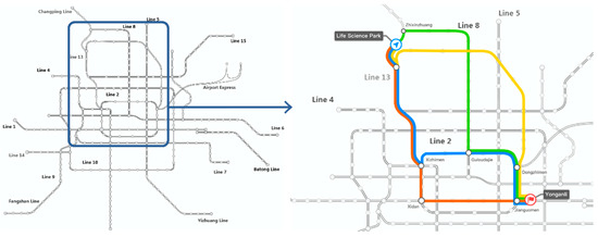
Figure 6.
The optimal strategy path from Life Science Park to Yonganli.
Life Science Park is on Line 13 and the destination Yonganli is on Line 1. The paths are represented in different colors. The red and blue paths share the same route until they reach Xizhimen Station, which is a transfer station for Lines 2 and 13. Line 2 is a ring line. Jianguomen is the transfer station for Lines 1 and 2. The two transfer stations are located diagonally in Line 2. The passengers can go clockwise or anticlockwise to reach their destination, which makes the red and blue paths. In the morning peak hour, the train frequency for the Line 13 clockwise direction is pretty high. Some passengers will choose the clockwise direction to reach Line 2 at Dongzhimen. After that, they finally get to the destination, which is the yellow path. In addition, the transfer walking distance in Guloudajie is shorter than the other transfer stations. Some passengers go in the clockwise direction and they transfer to Line 8 at Zhuxinzhuan Station, which is on the green path.
For some of the other OD pairs, they also have alternative paths during their trip. Although it is different from the previous OD pair, the paths are not in the clockwise or anticlockwise direction for the ring line. Take Renmin University to Dongdan as an example, as shown in Figure 7.
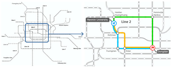
Figure 7.
The optimal strategy path for Renmin University to Dongdan.
Renmin University is on Line 4 and Dongdan is on Line 1. There are three paths in this OD pair. When the passengers reach Xizhimen by using Line 4, their total travel time may decrease if they transfer to Line 2. By doing this, some passengers might choose the blue path, and some will stay on Line 4 and transfer to Xidan Station, which is on the yellow path and it only transfers once. The train headway on Lines 5 and 10 is relatively small in the morning peak hour. Passengers may go upstream and transfer at Haidian Huangzhuang Station, which is the green path.
The optimal strategy path results show that many OD pairs have only one path, which is the shortest path. For some OD pairs, because of the train frequency and the transfer distance, the path that contains more transfers may have the potential to reduce the total travel time because the reduced transfer path may have a longer waiting time. The optimal strategy path can better illustrate the passenger flexibility in the network compared with the shortest path and the K-shortest path.
5. Discussion
The empirical study showed that the optimal strategy could be used in the complex transit network to demonstrate passenger behavior. Passengers, trying to follow the shortest path during their trip, could be verified from the data in Table 5. The proportion of the OD pairs that only contain the shortest path exceeded our expectations. When we mapped these OD pairs on our network, we found that some OD pairs are on the same line, which means passenger enter and exit at the same transit line. In this case, it is obvious that there is only a single shortest path, because every other path that contains transfers will only increase the travel time.
On the other hand, the operation strategy in Beijing metro is simple and straightforward, where the lines are mostly of the stop–stop operation. The complex skip–stop and through service operation plan are seldom applied in Beijing metro, which also leads to the results that most of the OD pairs only contain one path.
For the OD pairs that contain more than one path, we found that these OD pairs generally contain more than one transfer station. Because of the different transfer time at different transfer stations and the various train frequency on different transit lines, it is possible for passengers to switch to other paths and thereby reduce their total travel time, which explained the multiple transit paths for these OD pairs.
Furthermore, the number of reasonable paths is different for every OD pair. It is hard to determine a fixed K value in K-shortest path algorithm for all OD pairs in our transit network. On other hand, these results could better demonstrate the advantage of optimal strategy compared with the shortest path and K-shortest path. The optimal strategy could illustrate the passenger behavior in a more flexible way.
6. Conclusions
This study focused on the passenger’s path choice behavior in a complex transit network. The main conclusions of this paper are fivefold:
- (1)
- We reformed the optimal strategy as the optimal strategy tree to analyze the passenger’s behavior. Based on the optimal strategy results in Section 2, the passenger behavior could be taken as searching for the path along the optimal strategy tree.
- (2)
- The strategy node is defined. There is more than one attractive line/link starts within the strategy node, which determines the number of optimal strategy path.
- (3)
- The depth-first based optimal strategy path generation algorithm is proposed to illustrate passenger behavior. The algorithm complexity is highly dependent on the number of strategy nodes. The algorithm combines four parts: (a) initialization; (b) find optimal strategy link for the given node; (c) record path and path number; and (d) find the next optimal strategy node. The optimal strategy path could contain more than one shortest path.
- (4)
- The topology of the service network helps illustrate passenger behavior. The service network proposed some dummy nodes that represent the platforms and ticket gates are mapped to better illustrate the passenger’s precise boarding, alighting, waiting and walking behavior. The cost and frequency for each link is calibrated in seconds.
- (5)
- The path choice behavior analysis with the optimal strategy. Almost 80% of the OD pairs only have shortest path and less than 0.4% OD pairs have more than two paths. This calibration helps planners understand passenger behavior better and could be used in determining the K-shortest path. Based on the detailed analysis presented in Section 4.3.2, we found that, because of the different train frequencies and transfer times for some long-distance OD pairs, passenger may switch their path during the trip to reduce the total travel time.
This research, using the real AFC record data and timetables, provided a new method to infer the passenger path choice behavior. We determined that most of the OD pairs in the Beijing metro network only have one optimal path, which means that the passengers only follow the shortest path during their trip. This is because of the simple and fixed operation plan, which does not have a skip–stop operation and through service. Comparing with the given shortest path and K-shortest path behavior analysis, this method is more flexible and the number of reasonable paths differs from the OD pairs. In this way, the use of the fixed K value in the K-shortest path for all of the OD pairs in the network is not always reasonable.
Some aspects of this study could be improved by future research. Passengers may take more transfers to reduce their travel time. However, the transfer penalty is not considered in the optimal strategy model, which should be further discussed and researched. Moreover, we should apply the optimal strategy and the path generation algorithm in other cities, such as Shanghai and Guangzhou, to illustrate the validity of the model and the proposed algorithm solution. Passenger path choice and other behavioral characteristics can and should be better understood. Finally, if possible, we should explore flexible operation plans to make the passenger path choice more complete and analyze passenger behavior in a more comprehensive way.
Author Contributions
Conceptualization, K.L., T.T. and C.G.; methodology, K.L. and T.T.; formal analysis, K.L. and T.T.; writing—original draft preparation, K.L.; resources, C.G.; and supervision, C.G. All authors have read and agreed to the published version of the manuscript.
Funding
This work was supported by Beijing Postdoctoral Research Foundation (Award Number: ZZ2019-118).
Acknowledgments
The authors would like to thank Alireza Khani from the University of Minnesota and Zijia Wang from Beijing Jiaotong University for helping us edit and polish the language of this paper. We would like to thank Editage (www.editage.cn) for English language editing.
Conflicts of Interest
The authors declare no conflict of interest
Appendix A
The abbreviations in this research are listed as below.
Table A1.
The abbreviation in this research.
Table A1.
The abbreviation in this research.
| Abbreviation | Full Name |
|---|---|
| OD | Origin–Destination |
| AFC | Automatic fare collection |
| SBN | Schedule-based network |
| OSS | Optimal strategy set |
| SNL | Optimal strategy node-list |
| TNL | Temporary optimal strategy node-list |
| PSL | Path-set list |
| LN | Last node |
References
- Tong, C.O.; Richardson, A.J. A computer model for finding the time-dependent minimum path in a transit system with fixed schedules. J. Adv. Transp. 1984, 18, 145–161. [Google Scholar] [CrossRef]
- Gutenschwager, K.; Völker, S.; Radtke, A.; Zeller, G. The shortest path: Comparison of different approaches and implementations for the automatic routing of vehicles. In Proceedings of the Winter Simulation Conference, Berlin, Germany, 12 December 2012. [Google Scholar]
- Bander, J.L.; White, C.C. A new route optimization algorithm for rapid decision support. In Proceedings of the Vehicle Navigation and Information Systems Conference, Dearborn, MI, USA, 20–23 October 1991. [Google Scholar]
- Chabini, I.; Lan, S. Adaptations of the A* algorithm for the computation of fastest paths in deterministic discrete-time dynamic networks. IEEE Trans. Intell. Transp. 2002, 3, 60–74. [Google Scholar] [CrossRef]
- Zhou, W. Improved Dial Algorithm for Urban Rail Transit Path Selection. J. Xihua Univ. (Nat. Sci. Ed.) 2013, 32, 38–40. [Google Scholar]
- Dial, R.B. A probabilistic multi-path traffic assignment mode1 which obviates path enumeration. Transp. Res. 1971, 5, 83–111. [Google Scholar] [CrossRef]
- Hershberger, J.; Maxel, M.; Suri, S. Finding the K-shortest simple paths: A new algorithm and its implementation. ACM Trans. Algorithms 2007, 3, 45. [Google Scholar] [CrossRef]
- Li, J. Study on the Passenger Flow Assignment Model and Algorithm of Urban rail Transit Network. Master’s Thesis, Beijing Jiaotong University, Beijing, China, 2010. [Google Scholar]
- Xu, R.; Luo, Q.; Gao, P. Passenger flow distribution model and algorithm for urban rail transit network based on multi-route choice. J. Chin. Railw. Soc. 2009, 31, 110–114. [Google Scholar]
- Liu, Q. The Research and Implementation of Guidance System of Passenger Flow on Urban Rail Transit. Master’s Thesis, Beijing Jiaotong University, Beijing, China, 2009. [Google Scholar]
- Liu, J.F.; Sun, F.L.; Bai, Y.; Xu, J. Passenger flow route assignment model and algorithm for urban rail transit network. J. Transp. Syst. Eng. Inf. Technol. 2009, 9, 81–86. [Google Scholar]
- Gen, M.; Cheng, R.; Wang, D. Genetic algorithms for solving shortest path problems. In Proceedings of the 1997 IEEE International Conference on Evolutionary Computation, Indianapolis, IN, USA, 13–16 April 1997. [Google Scholar]
- Hamed, A.Y. A genetic algorithm for finding the k shortest paths in a network. Egypt Inf. 2010, 11, 75–79. [Google Scholar] [CrossRef]
- Fan, W.; Machemehl, R.B. Using a simulated annealing algorithm to solve the transit route network design problem. J. Transp. Eng. 2006, 132, 122–132. [Google Scholar] [CrossRef]
- Niksirat, M.; Ghatee, M.; Hashemi, S.M. Multimodal K-shortest viable path problem in Tehran public transportation network and its solution applying ant colony and simulated annealing algorithms. Appl. Math. Model. 2012, 36, 5709–5726. [Google Scholar] [CrossRef]
- Cheng, Z.; Sun, Y.; Liu, Y. Path planning based on immune genetic algorithm for UAV. In Proceedings of the 2011 International Conference on Electric Information and Control Engineering, Wuhan, China, 15–17 April 2011. [Google Scholar]
- Yang, L.; Lin, J.; Wang, D.; Jia, L. Dynamic route guidance algorithm based on artificial immune system. J. Control. Theory Appl. 2007, 5, 385–390. [Google Scholar] [CrossRef]
- Mahi, M.; Baykan, Ö.K.; Kodaz, H. A new hybrid method based on particle swarm optimization, ant colony optimization and 3-opt algorithms for traveling salesman problem. Appl. Soft. Comput. 2015, 30, 484–490. [Google Scholar] [CrossRef]
- Papadimitriou, F. The Algorithmic Complexity of Landscapes. Landsc. Res. 2012, 37, 599–611. [Google Scholar] [CrossRef]
- Papadimitriou, F. Mathematical Modelling of Land Use and Landscape Complexity with Ultrametric Topology. J. Land. Use Sci. 2013, 8, 234–254. [Google Scholar] [CrossRef]
- Derrible, S.; Kennedy, C.E.J. The complexity and robustness of metro networks. Phys. A 2010, 389, 3678–3691. [Google Scholar] [CrossRef]
- Khani, A.; Hickman, M.; Noh, H. Trip-based path algorithms using the transit network hierarchy. Netw. Spat. Econ. 2015, 15, 635–653. [Google Scholar] [CrossRef]
- Huang, R.; Peng, Z.R. Schedule-based path-finding algorithms for transit trip-planning systems. Transp. Res. Rec. 2002, 1783, 142–148. [Google Scholar] [CrossRef]
- Friedrich, M.; Hofsäß, I.; Wekeck, S. Timetable-based transit assignment using branch and bound techniques. Transp. Res. Rec. 2001, 1752, 100–107. [Google Scholar] [CrossRef]
- Niu, X.; Pan, Y. Urban rail transit assignment algorithms. Comput. Era 2005, 2, 17–18. [Google Scholar]
- Fredman, M.L.; Tarjan, R.E. Fibonacci heaps and their uses in improved network optimization algorithms. J. ACM 1987, 34, 596–615. [Google Scholar] [CrossRef]
- Xu, R.; Li, W.; Zhu, W. Path Set Generation Algorithm for Schedule based Rail Transit with Constraints of Time and Space. Tongji Daxue Xuebao 2015, 43, 1025–1030. [Google Scholar]
- Yang, Y.; Yan, Y.S.; Hu, Z.A.; Ma, Y. Improved Dial’s Algorithm for Logit-Based Stochastic Traffic Assignment Model. J. Transp. Syst. Eng. Inf. Technol. 2013, 13, 158–163. [Google Scholar]
- Spiess, H.; Florian, M. Optimal strategies: A new assignment model for transit networks. Transp. Res. B-Methodol. 1989, 23, 83–102. [Google Scholar] [CrossRef]
- Lu, K. Optimal Strategy Based Passenger Simulation and Behavior Inference for Urban Rail Transit. Ph.D. Thesis, Beijing Jiaotong University, Beijing, China, 2019. [Google Scholar]
- Wikipedia: Breadth First Search. Available online: https://en.wikipedia.org/wiki/Breadth-first_search (accessed on 11 December 2019).


© 2020 by the authors. Licensee MDPI, Basel, Switzerland. This article is an open access article distributed under the terms and conditions of the Creative Commons Attribution (CC BY) license (http://creativecommons.org/licenses/by/4.0/).