Evaluation of Two Improved Schemes at Non-Aligned Intersections Affected by a Work Zone with an Entropy Method

Abstract

The impact of work zones on traffic is a common problem encountered in traffic management. The reconstruction of roads is inevitable, and it is necessary and urgent to reduce the impact of the work zone on the operation of traffic. There are many existing research results on the influence of highway work zones, including management strategies, traffic flow control strategies, and various corresponding model theories. There are also many research results on the impacts of urban road and subway construction on traffic operation, including construction efficiency, economic impact, and travel matrix. However, there are few studies concerning the choice of work zone location, and most previous studies have assumed that the work zone choice was scientific and reasonable. Therefore, it is reasonable to choose the location of the work zone and to assess whether there is room for improvement in the road form of the work zone, but this remains a research gap. Therefore, we studied a seven-lane main road T-intersection in Xi’an, China, and investigated a work zone located at this intersection that caused a road offset, leading to the non-aligned flow of main traffic. We designed two road improvement schemes and multiple transition schemes, used VISSIM software to evaluate the traffic operation of the two schemes, and used the entropy method to choose the suitability of the two schemes under different conditions. According to the results, in the best case, the driving time, delay, and number of stops are reduced by 44%, 66%, and 92%.

1. Introduction

Sustainable traffic flows through intersections have long been regarded as the central issue in urban transportation systems. Inbound traffic flows from different directions merge and diverge at intersections, which are often disturbed for various reasons, leading to traffic congestion. The intersection traffic problem not only causes congestion, but also generates air pollution [1] and potential safety hazards [2]. Restriction policies and congestion charges are also results of congestion [3]. Not all intersections are standard, which can be the results of urban scheming, building near the intersection, imbalance between the number of lanes, road markings, and traffic optimization [4,5,6]. Cross intersections [7] and T-intersections [8] are commonly used shapes, whereas roundabouts [9,10] and unconventional intersections [11] are not rarely seen. All these forms of intersections affect traffic operations to different degrees [12]. Many researchers have achieved major successes in improving intersection operations, including methods for the control of left-turn traffic [13], timing of traffic lights [14,15], optimization of road channelization [16], and control of U-turn vehicles [17]. Left-turn traffic has been the focus of much research, because movement in this direction has the greatest impact on the capacity of intersections [18,19]. However, in practice, non-aligned intersections are the result of various circumstances and affect through-traffic operation, where through-traffic operation is often ignored.

The effects of work zones or work zone settlements worsen non-aligned intersections. People often think that traffic congestion at non-aligned intersections is natural or inevitable for objective reasons. In particular, work zones such as subway construction in cities occupying a part of the intersection generate a non-aligned road on the two sides. This kind of work zone remains for a long time, which may be several months or even years, and significantly impacts traffic operation.

Therefore, this paper mainly studies the non-aligned intersection caused by work zones occupying intersections. The research on impacts of the work zone concentrates on two major categories. One is the freeway work zone impact, including the influence of capacity [20], work zone influence area [21], and traffic flow prediction models [22], and so forth. The other category is the urban work zone impact, such as the urban travel OD matrix [23], alternative route selection studies [24], and traffic organization management [25], and so forth. While existing studies lack research on the work zone layout and corresponding road geometric layout, few research papers have focused on the rationality of the work zone layout and corresponding road layout. However, the unsuitable work zone settlement and road layout could also have a negative effect on sustainable flow operation. This paper takes the subway work zone of a main road T-intersection in Xi’an, China as an example. Taking the intersection road geometric design and work zone layout as the research content, we propose two work zone layouts and corresponding intersection road layouts when the work zone is set at the intersection. Field survey data and the VISSIM simulation and entropy evaluation method are used to calculate and evaluate the two schemes. The best scheme under different volume combinations is selected, which is of great significance for improving the traffic operation status of intersections and reducing the impact of work zones on urban traffic flow.

The non-aligned intersection discussed in this article is very similar to the dual T-intersection under some circumstances. The two kinds of intersections are easily confused, but they are completely different, as shown in Figure 1. For the dual T-intersection, the operation problem is mainly caused by the distance between two adjacent T-intersections. Two adjacent T-intersections are connected by a short segment and controlled by two traffic lights (one in each intersection), which can be synchronous or asynchronous. The non-aligned intersection mentioned here means that two sides of the roads are not in a straight line at one intersection. No extra segment connects the two sides, and only one traffic light controls the intersection. The main concern under this circumstance is that the through-traffic is offset when passing through the intersection.

The remainder of this article is organized as follows: Section 2 surveys the literature; Section 3 introduces the problem statement, data collection, and calibration of the simulation model; Section 4 introduces solutions and analyzes the performance of two improved schemes; Section 5 discusses the comparison of the two improved schemes with the entropy method, where a final selection matrix is calculated, and the difference between the two schemes is also introduced; and Section 6 concludes the paper.

2. Literature Review

2.1. Highway Work Zone Impact

Non-aligned intersections are the result of various circumstances, such as urban planning, non-aligned road markings, and construction effects. Some results on the impact and corresponding measures of work zones on traffic operation have been reported [20]. Most of the achievements related to work zone influence are focused on highway work zones. Ideally, traffic managers can inform drivers of alternative routes around the work zone in advance of the project location when temporary closures are caused by highway construction. According to a survey conducted in Puerto Rico, when highway drivers pass through a work zone, at least 50% of them are distracted. Furthermore, drivers tend to comply with work-zone speed limits when personnel or heavy equipment are present in the area [21]. The influence of a highway work zone on safety differs between the daytime and nighttime, while older male drivers, the number of lane closures, sidewise crashes, and rainy weather have opposite effects on the severity of crash-related injuries at night compared with crashes in the daytime [26].

2.2. Predict and Evaluate Method of Highway Work Zone Impact

Some researchers have developed different methods to predict and evaluate the impact of construction on traffic operation, such as dynamic traffic assignment [27], a five-parameter logistic model that describes the speed–density relationship [22], an optimal nonlinear fitting theory [28], traffic speed versus flow curves, capacity reduction factors, and free-flow speed reduction factors [29]. A bilevel optimization model was proposed for the purpose of minimizing the total travel time of the affected network, involving a link closure and a proposed alternate route for travelers [30]. With a cellular automata model, a highway was divided into the normal area, merging area, and work zone, and the suitable merging length and the appropriate speed limit value were found to be key factors for managing work zone traffic operation [31]. A dynamic control model was used to optimize the signal operations of a new merging system, the lane-based signal merge (LBSM), which uses lane-based signals or variable signs to give drivers in different lanes the right-of-way to proceed through the open lane(s) in a work zone area [32]. A simulation-based analysis is more appropriate for network analysis, for long corridors, for signalized arterials, or for cases in which congestion of the arterial network significantly affects freeway operations [33].

2.3. Urban Roads and Subway Work Zone

Besides highway work zone control models, the effects of urban roads and subway construction have also received attention from researchers. In an urban area, a subway work zone has a direct influence on the surrounding road network. Origin Destination (OD) matrix estimation was distributed on a road network with TransCAD to evaluate the traffic organization scheme. The service level of roads and intersections were found to be evaluation indicators that could reduce traffic influence on a road network during subway construction [23]. Combined with the OD distribution principle, the traffic impact of the construction section was analyzed, and the scope of influence was determined. The average delays, queue length, and number of vehicles were selected as three indexes, and VISSIM was used for the simulation of guidance measures to evaluate a better traffic organization scheme [34]. Portable changeable message signs (PCMSs) have been used in work zones to increase legibility. Graphic-aided PCMSs reduced the mean vehicle speed by between 13% and 17% and reduced the speed of passenger cars and trucks significantly differently depending on their locations in a work zone [24]. For reconstruction scheme evaluation, the level of service, negative economic benefit, and traffic environmental impact can be used as analysis and screen indexes. An integrated approach, combined with a dynamic comprehensive evaluation and the analytic hierarchy process was proposed to evaluate traffic organization during highway construction [35]. A survey conducted in New York City showed that the saturation flow rate per lane increased during the work zone. Although the overall approach capacity decreased because a lane was closed, it did not decrease as much as expected [25].

2.4. Methods for Work Zone Impact Research

To reduce the negative impact of construction, simulation is one of the best ways to evaluate measurements before their application. A larger system simulation of a Hong Kong microtunneling and pipe-jacking operation concluded that a balance between construction productivity and traffic mobility could be maintained through appropriate truck delivery routes; the timing, sizing, and location of a temporary laydown area; the traffic lane closure distance; and work scheduling [36]. Urban subway construction increased the travel time delays, queue length, fuel consumption, number of forced merges, and roadway accidents. The use of VISSIM to calculate economic losses and to specify systematic work zone schedules and traffic management techniques is necessary [37].

There have recently been some new technologies, such as the intelligent transportation system (ITS) [38,39,40], autonomous vehicles [41], and advanced driving simulator [42]. A multilayer feed-forward artificial neural network (ANN) model could be used to track drivers and vehicles in work zones; the new model performs better than the traditional deterministic queuing model in estimating the travel delay caused by the work zone [43]. One of the future technologies is the connected vehicle. Work zone operation could benefit from this technology as a result of the travel time and its reliability [44]. Some elements of traffic operation are sometimes ignored, such as the impact of construction equipment. Construction equipment can also cause traffic congestion, especially in the bottleneck section; and conversely, unsustainable traffic operation influences the efficiency of the equipment used in the construction schedule [45].

Channelization is a popular and effective method used to reduce traffic problems [46]. An exclusive left-turn lane can be used when left-turn vehicles make up a high proportion of the whole flow [47]. Left-turn lanes can reduce the number of crashes with the opposing through-traffic [48,49]. A left-turn waiting area could also improve the capacity at the intersection [50]. Signalization is another popular control method at intersections [51,52]. An exclusive left-turn phase can be used for heavy left-turn vehicles [53,54]. Left-turn control has been found to significantly improve the operational conditions in China [55,56,57]. Other types of intersections are also used to reduce intersection problems [58].

The learning from the literature review indicates that the existing research results from the influence of highway work zones, including management strategies, traffic flow control strategies, and various corresponding model theories. There are also many research results on the impact of urban road and subway construction on traffic operation, including construction efficiency, economic impact, and travel matrix. However, there are few studies concerning the choice of work zone location, and most previous studies have assumed that the work zone choice was scientific and reasonable. Therefore, it is reasonable to choose the location of the work zone and to assess whether there is room for improvement in the road form of the work zone, but this remains a research gap.

3. Problem Statement and Data Collection

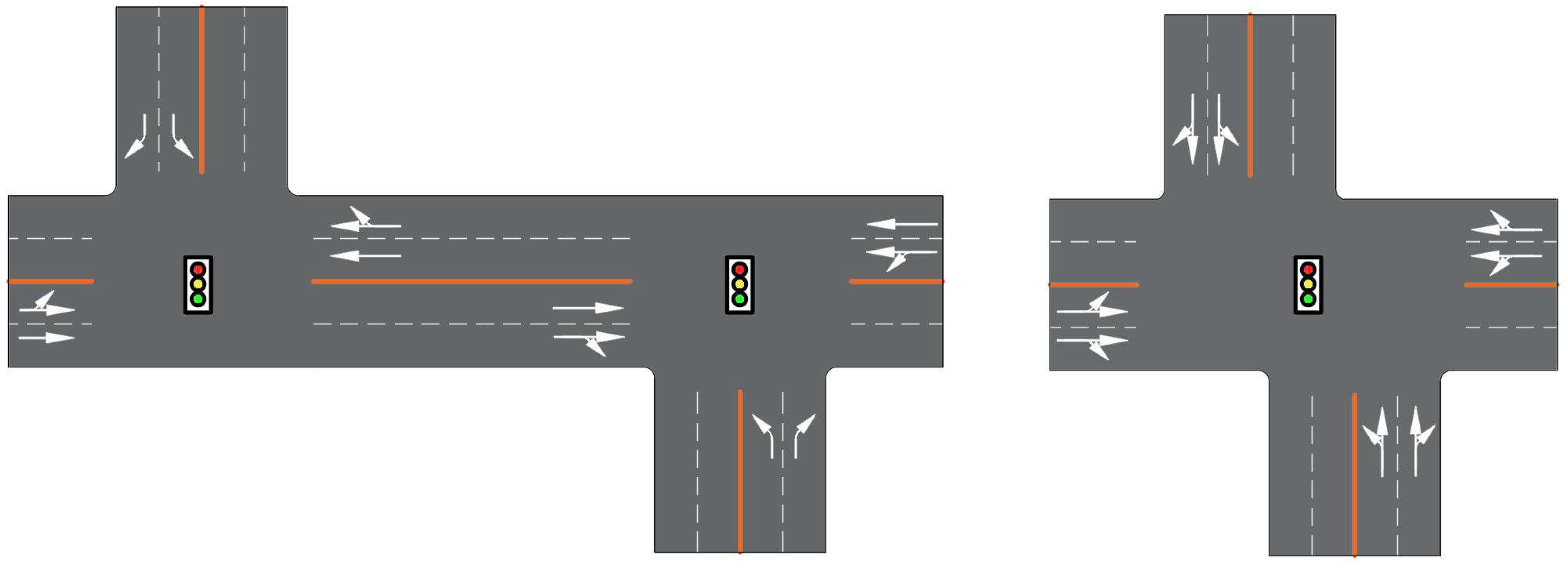
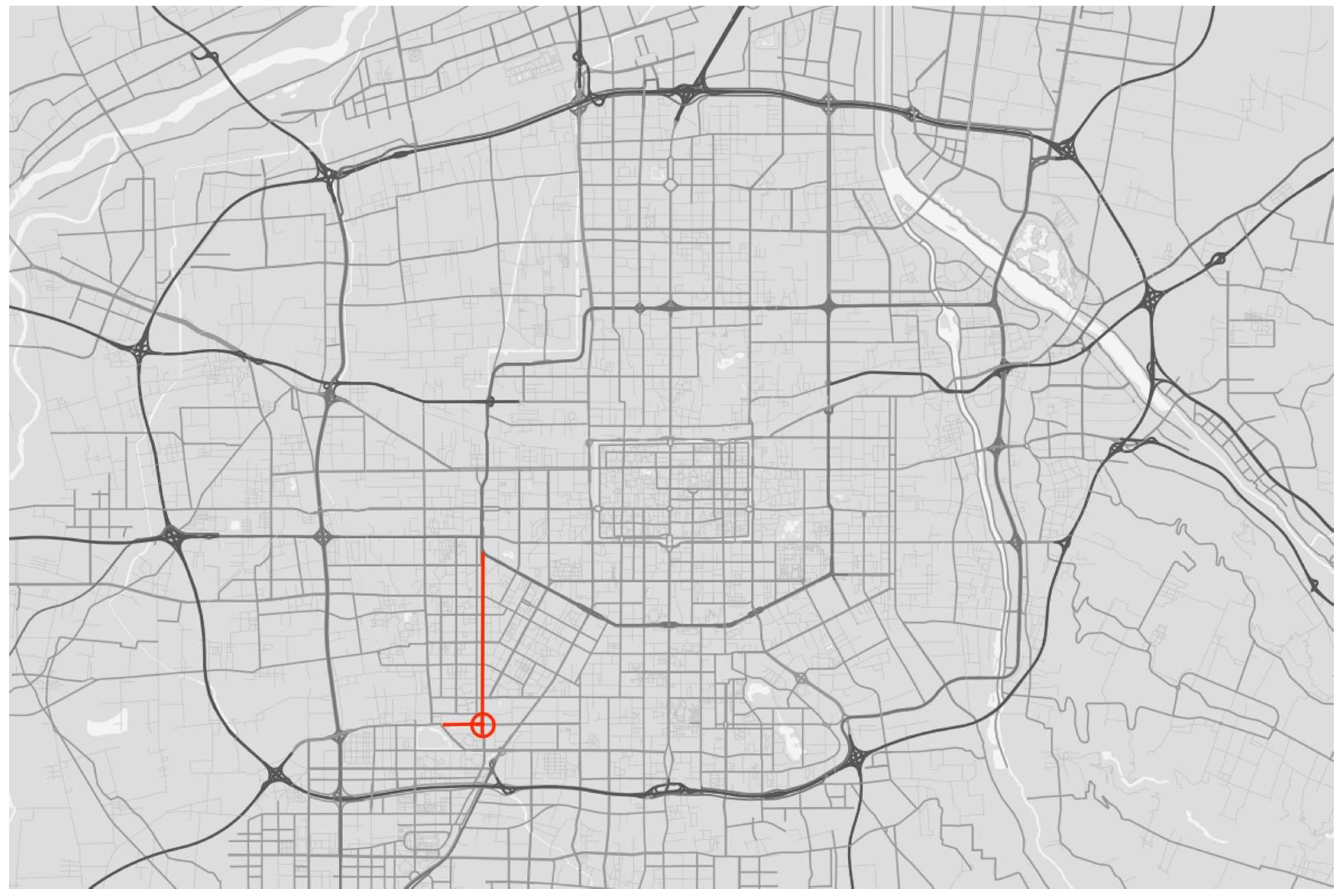
3.1. Problem Statement

Xi’an City is taken as an example in this study. At the end of 2018, the population of Xi’an was more than 10 million, and the number of vehicles was 3.25 million [59]. Furthermore, Xi’an has a history of more than 3100 years [60] and massive historical relics, which have resulted in a long construction period in this district [61]. The selected T-intersection is located at the main avenue in the central position of a business area, as shown in Figure 2. The North–South arterial street was a 12-lane road, but it is now a seven-lane road (three lanes Southbound and four lanes Northbound) and connected to the West by a seven-lane collector street (four lanes Westbound and three lanes Eastbound). The distances to adjacent intersections are 270 m, 1100 m, and 720 m to the North, West, and South, respectively.

As Figure 3 shows, the intersection is occupied by a work zone in the northern part of the intersection. The stop lines between the South and North are 47 m apart, and the offset distance is 28 m. The vehicles can move in each direction of the T-intersection with no restrictions. Each direction of the three traffic flows is controlled by one traffic light, and no exclusive left-turn traffic light exists.

Because of the large area of the intersection and heavy traffic, the South–North flow often forms additional flows on both sides of the original three-lane flow when passing through the intersection. The West–North flow also fills up all the potential left-turn paths as much as possible and tries to pass through the zone that conflicts with North–South traffic as quickly as possible. The two Northbound traffic flows merge together, and other flows are smooth (Figure 3).

3.2. Data Collection

The collection of real traffic data is necessary to build and calibrate the simulation model in VISSIM. Field data collection was conducted during both peak and valley hours on weekdays and the weekend. According to an investigation, the traffic volume of this intersection on the weekend was much less than that on weekdays. The congestion index in the top 50 cities can be gathered from the AutoNavi Traffic Company [62]. The morning peak appeared from 7:00 a.m. to 9:00 a.m., and the evening peak appeared from 5:00 p.m. to 7:00 p.m. The 24-hour congestion index in Xi’an on 17 January 2019 is shown in Figure 4.

The collected data are as follows:

• Speed and types of vehicles in each lane;
• Turning vehicles, including left turns and right turns;
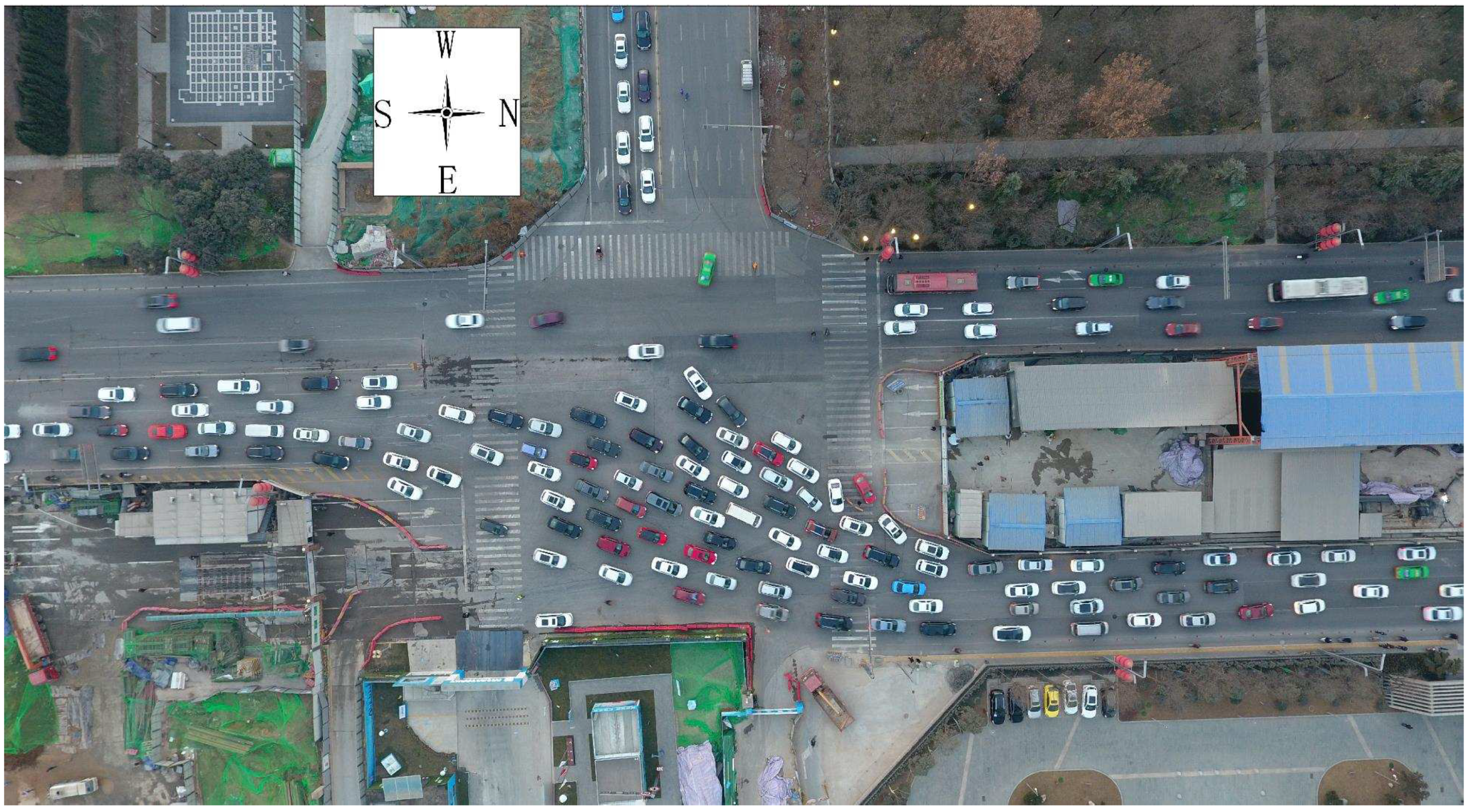
• Vehicle behavior in the intersection area, especially the South–North vehicle chaos.

The collected volume during the morning peak hour was 6333 veh/h, the volume during the middle noon valley was 5895 veh/h, while the volume during the evening peak hour was 6825 veh/h. Thus, the peak-hour data were selected as the representative. The collected data of the peak periods in 1 h are listed in

Table 1. Collected data during one peak hour, from 5:00 p.m. to 6:00 p.m. on 17 January 2019.

Item	South to North		North to South		Eastbound
Flow	Through	Left turn	Through	Right turn	Left turn	Right turn
Flow Number	$i=1$	$i=2$	$i=3$	$i=4$	$i=5$	$i=6$
Car	3170	59	2599	118	511	130
Truck/Bus	135	0	81	0	10	0
Max. speed (km/h)	22.4	25.1	65.2	26.3	22.2	23.2
Min. speed (km/h)	0	0	0	0	0	0
Average speed (km/h)	17.3	16.4	31.7	19.8	14.3	20.6

The minimum speed of 0 km/h means that vehicles were stopped and then moved.

.

The collected data show the following characteristics:

1.

The average speed of Flow $i=3\&4$ was much higher than that of Flow $i=1\&2$, and the offset of trajectories strongly affected vehicle operation.

2.

Neither Flow $i=2$ nor Flow $i=4$ was affected by the offset.

3.

The collector street volume was much less than the arterial street volume, the operation of which was hardly affected by the offset.

The collected trajectories in Figure 5 show the following characteristics:

1.

Northbound vehicles (Flow $i=1\&5$) were crowded in the intersection area, whereas the Southbound (Flow $i=3\&6$) and Westbound (Flow $i=2\&4$) vehicles were hardly affected.

2.

Lane D is a left-turn lane, but through-vehicles used it when other lanes were crowded.

3.

Lane E is a right-turn lane, but left-turn vehicles used it when other lanes were crowded, and some of the left-turn vehicles of lane E detoured via the outside route to avoid the queue.

4.

The outside vehicles operated faster than the inside vehicles; the inside vehicles needed to merge with other vehicles, which caused the delay.

5.

According to the investigation, vehicles of lane G preferred to turn left with a small radius, which was the inside lane when turning left. However, all inner five or six lines of the vehicles had to merge into only one single lane, and because it was difficult to change to the adjacent lane, the inner vehicles moved very slowly. On the basis of observation, the longest time taken by a vehicle of Flow $i=5$ to pass through the intersection was about 6 min.

3.3. Calibration of the VISSIM Simulation Model

In order to increase the accuracy of the VISSIM simulation model in the following steps, calibration was needed before the sensitivity analysis. The collected traffic data, signal cycles, and road geometry were all calibrated with the collected traffic volume. A standard calibration procedure proposed by previous studies was followed [63,64,65,66]. The parameters of the intersection input into the VISSIM model were as follows:

1.

The ratio of trucks and cars collected from Table 1;

2.

The volume of each flow collected from Table 1;

3.

The speed of each flow collected from Table 1;

4.

The traffic light cycle of the intersection;

5.

The geometric parameters of the intersection.

A car-following model, gap-accepting model, and lane-changing model are all available for the VISSIM calibration, but volume capacity is the most commonly used index for calibration. Capacity accuracy is required, and it reflects the VISSIM model accuracy with high sensitivity. The capacity is calculated according to Equation (1):

$$C=\frac{3600}{\overline{{\mathrm{h}}_{\mathrm{t}}}},$$

(1)

where C denotes the ideal capacity (veh/h), and $\overline{{\mathrm{h}}_{\mathrm{t}}}$ is the average minimum headway (s). An index named Mean Absolute Percent Error (MAPE) can reflect the error between the simulation capacity and collected volume. The MAPE can be calculated by Equation (2):

$$MAPE=\frac{{\displaystyle \sum _{i=1}^n{C}_v^i-\sum _{i=1}^n{C}_f^i}}{{\displaystyle \sum _{i=1}^n{C}_f^i}},$$

(2)

where n denotes six-direction flows, $C_v^i$ is the VISSIM simulated capacity (veh/h), and $C_f^i$ is the volume according to investigation (veh/h). The calculated MAPE is displayed in

Table 2. VISSIM simulation calibration results with collected data for three periods.

	Flow	$\mathit{i}=1$	$\mathit{i}=2$	$\mathit{i}=3$	$\mathit{i}=4$	$\mathit{i}=5$	$\mathit{i}=6$
Morning peak data	Investigated capacity (veh/h)	3074	54	2492	109	484	120
	Simulated capacity (veh/h)	2865	58	2237	87	495	134
	Individual MAPE (%)	−6.8	5.7	−10.2	−20.7	2.1	10.8
	MAPE (%)	−7.3
Middle (noon) valley data	Investigated capacity (veh/h)	2985	37	2658	37	149	29
	Simulated capacity (veh/h)	2649	45	2214	32	159	34
	Individual MAPE (%)	−11.3	21.6	−16.7	−13.5	6.7	17.2
	MAPE (%)	−12.9
Evening peak data	Investigated capacity (veh/h)	3305	59	2680	118	521	130
	Simulated capacity (veh/h)	3174	65	2387	94	545	146
	Individual MAPE (%)	−4.0	10.1	−10.9	−20.3	4.6	12.3
	MAPE (%)	−5.9

:

The MAPEs of the three periods are −7.3%, −12.9%, and −5.9%, respectively, and these values suggest that the calibration accuracy of the VISSIM model is reasonable. According to previous studies, this error can be accepted [67,68].

3.4. VISSIM Calculation of Operational Measures

The most commonly used indexes for evaluating the improvement of traffic programs with different operational volumes are travel time, delay, and the number of stops [69,70]. The calculation of these indexes is as follows:

Travel time. Travel time is the time that it takes for all vehicles to pass through the intersection in the simulation. It is the calculated time from appearance at the upper section of the road to disappearance at the end of the road in the simulation. It can be calculated as Equation (3):

$$T_{{}_i}^k=\frac{{\sum }_{j=1}^{Q_i^k}{t}_{{}_{ij}}^k}{Q_i^k}\forall i=1,2,3,4,5,6\forall k=1,2,\dots ,etc.,$$

(3)

where $T_{{}_i}$ denotes the travel time of each direction of traffic flow in Table 1, $t_{{}_{ij}}$ denotes the travel time of each vehicle, $Q_i$ denotes the number of total vehicles of each flow, $k=1$ denotes the present intersection situation, and $k=2,\dots ,etc.$ denotes the different improved schemes in the simulation.

Delay. A difference always exists between a driver’s arrival time and expected time. Traffic interference, traffic control, and management are all possible reasons for a delay. The stop delay and travel delay are both included in the simulation:

$$D_i^k=d_{i1}^k+d_{i2}^k\forall i=1,2,3,4,5,6\forall k=1,2,\dots ,etc.,$$

(4)

where $D_i$ denotes the whole delay of each direction’s flow in Table 1, $d_{i1}$ and $d_{i2}$ represent the stop delay and travel delay of each flow, respectively, and $k=1$ and $k=2,\dots ,etc.$ represent the present and different improved situations, respectively.

Number of stops. All standstill situations (speed = 0) in the VISSIM consist of the number of stops, and parking lots or bus stops are not included. It can be calculated by the total number of stops divided by the total number of vehicles:

$$S_{{}_i}^k=\frac{{\sum }_{j=1}^{Q_i^k}{s}_{{}_{ij}}^k}{Q_i^k}\forall i=1,2,3,4,5,6\forall k=1,2,\dots ,etc.,$$

(5)

where $S_{{}_i}^k$ denotes the average number of stops in Table 1, $s_{{}_{ij}}$ denotes the number of stops of each vehicle, and $Q_i$ is the total number of stops. $k=1,2,\dots ,etc.$ denotes the present situation and different improved situations.

4. Solutions and Analysis

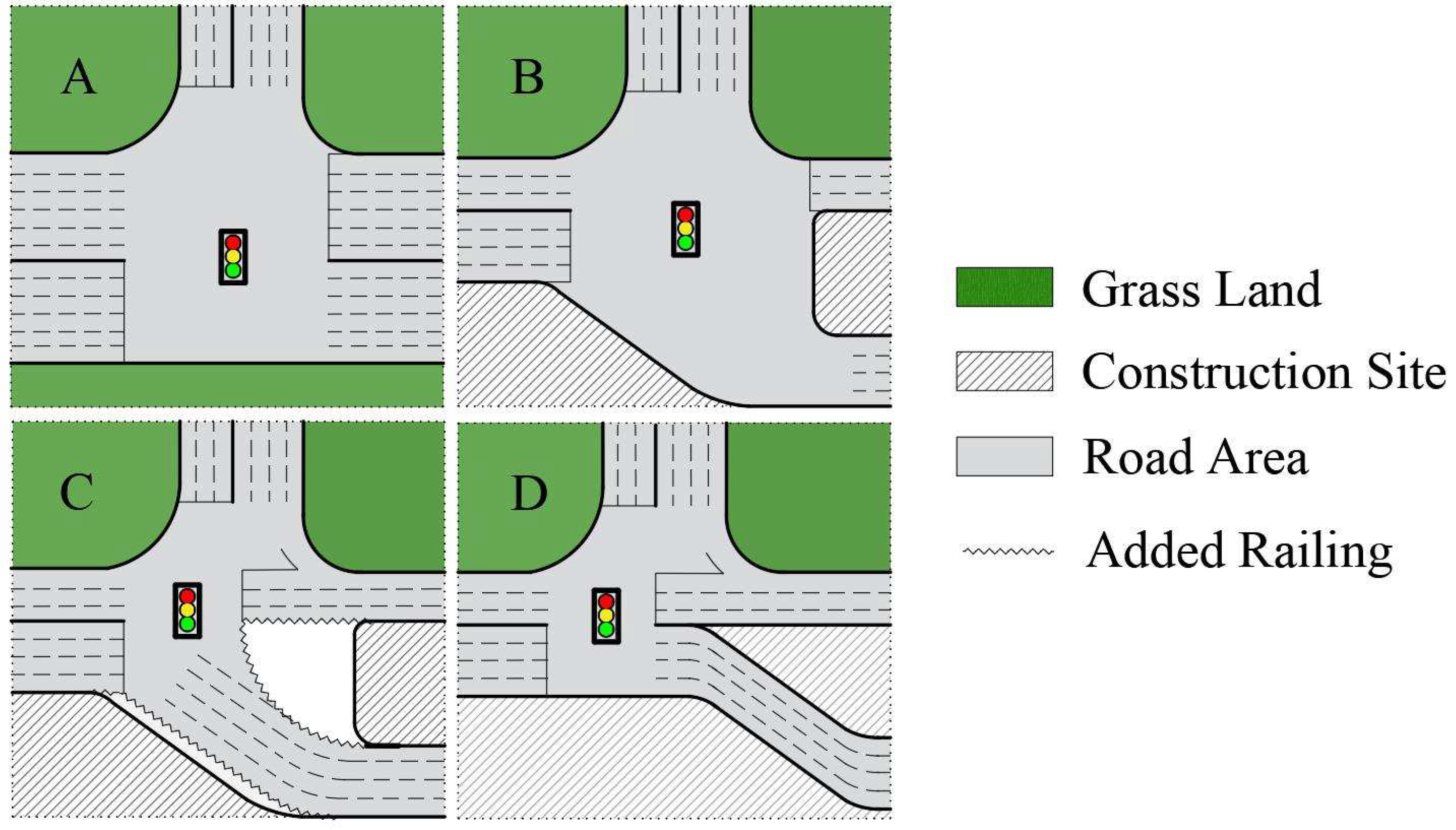
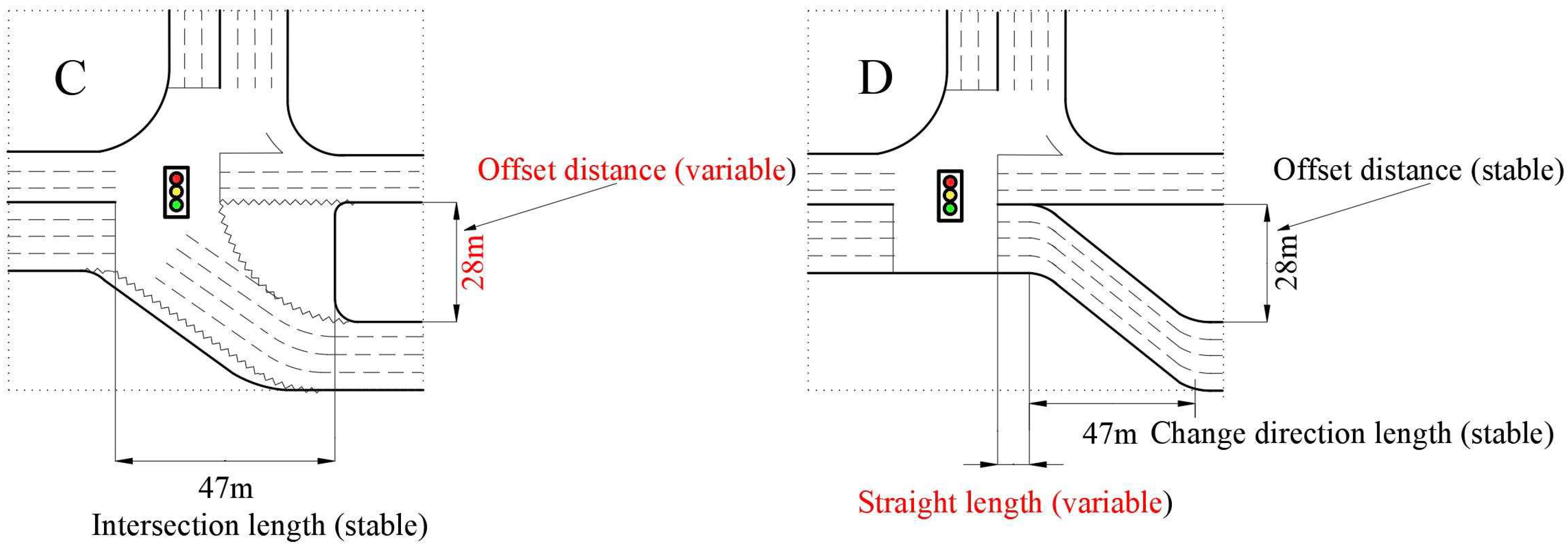
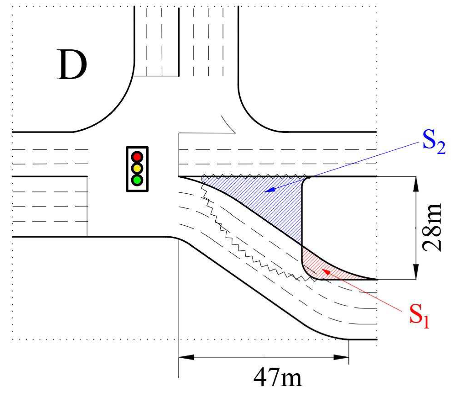
4.1. Solutions

According to Figure 3 and Figure 5, the reason for the congestion at this intersection is the vehicle merge movement on the inner side. Northbound traffic flow is restricted by the road width and lane markings on both sides of the intersection. The driving width is much wider than four lanes when vehicles pass through the intersection. When the front vehicle decelerates or changes a lane, the following vehicles decelerate, change a lane, or attempt to bypass the front vehicle from the outside. This movement can fill the whole intersection area, and then vehicles are slowly squeezed forward.

The core reason for congestion is that a wide intersection area with a maximum 11-lane width narrows into a four-lane width. To reduce the traffic congestion and improve the operational features, channelization is the key solution. Keeping operating vehicles within the lines in the intersection area was the main purpose of the solutions.

Figure 6A is the original situation of the intersection before the construction starts. Both sides of the intersection are 12 lanes. Figure 6B is the present situation, in which the work zone occupies two parts of the intersection. The southern part narrows, and the northern part of the intersection is divided. Figure 6C is based on the present situation, with some railing added to narrow the intersection area, restrict vehicle operation to no wider than four lanes, and reduce the inner queue in order to keep vehicles in the lines when passing through the intersection. Figure 6D is another possible solution to improve the intersection. Vehicle operation is kept in a straight line to avoid the influence of the work zone, and then vehicles change direction as the road alignment changes.

The 28 m offset of this intersection results in traffic delay and congestion. Would the operation situation improve if the offset was less than 28 m? Is there any relationship between the offset value and traffic operation? In order to find out the relation, different offset situations were evaluated, as shown in Figure 7. The offset value is 28 m, and the different offset values in the simulations were 0∼28 m with a step size of 2 m. The solution of scheme D was also evaluated with different straight lengths after the intersection, followed by a turning direction. The straight length was simulated in a range from 0 to 100 m with a step size of 10 m.

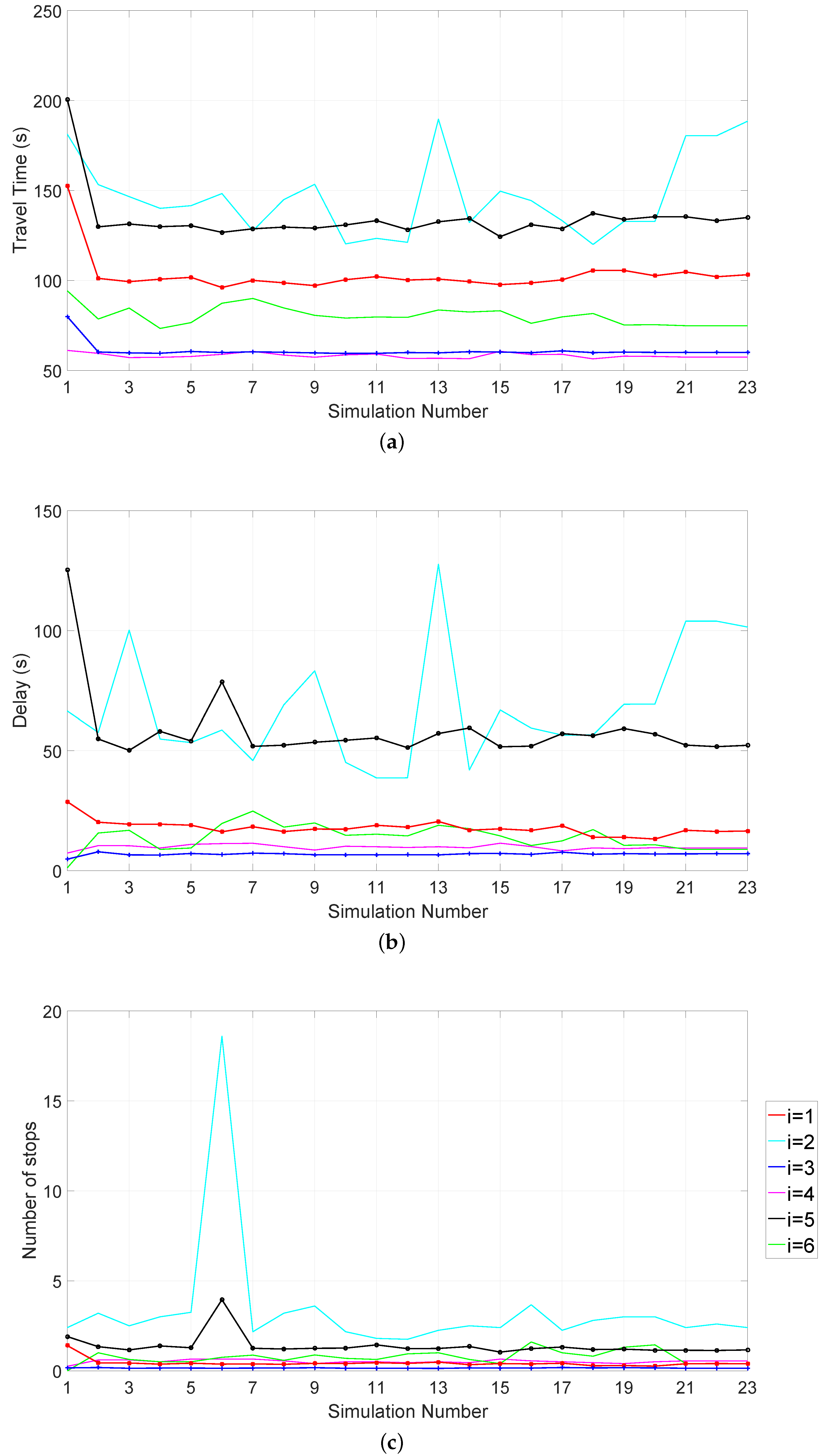
4.2. Simulation Result

There were 23 simulations in total: the present situation (Figure 6B), 15 offset simulations (Figure 6C), and straight length simulations (Figure 6D) with 0 m, 10 m, 20 m, 30 m, 40 m, 50 m, and 100 m. The collected data in Table 1 were input into VISSIM simulation models to evaluate the different solutions for the same volume. The results are reported below.

It is evident that the present simulation result, group Scheme 1 in the three figures in Figure 7, is much higher than the other situations. The main traffic flows in the six directions are $i=1$, $i=3$, and $i=5$. They all have a similar trend that fluctuates in a small range and almost maintains a straight line. This indicates that the difference resulting from changing the offset value or extending the straight length has little influence on the results. The other three traffic flows have pronounced fluctuations but no clear patterns. This cannot indicate whether the different improvement schemes can promote or inhibit the operation.

4.3. Safety Evaluation

A complete evaluation should conclude with an operation and safety evaluation. A commonly used tool, the surrogate safety assessment model (SSAM), is a simulation and analysis project of the Federal Highway Administration (FHWA) to predict the safety of roadways before crashes occur. The SSAM is a software application developed to automatically identify, classify, and evaluate traffic conflicts in the vehicle trajectory data output from microscopic traffic simulation models. The SSAM also has built-in statistical analysis features for conflict frequency and severity measures that can aid analysts in the design of safe traffic facilities [71,72,73]. The safety analysis was applied to 23 schemes with evening peak hour data, where the results are shown below in

Table 3. Safety analysis of 23 simulations by SSAM.

Scheme Number	Item	Crossing	Rear End	Lane Change	Total
1	Present situation	362	609	102	1073
2	Offset 0 m	1	123	48	172
3	Offset 2 m	0	118	63	181
4	Offset 4 m	0	232	83	315
5	Offset 6 m	0	142	69	211
6	Offset 8 m	0	165	68	233
7	Offset 10 m	0	162	67	229
8	Offset 12 m	1	151	71	223
9	Offset 14 m	1	133	63	197
10	Offset 16 m	0	165	85	250
11	Offset 18 m	0	177	96	273
12	Offset 20 m	0	151	66	217
13	Offset 22 m	0	155	63	218
14	Offset 24 m	0	139	85	224
15	Offset 26 m	0	131	80	211
16	Offset 28 m	1	207	62	270
17	Straight 0 m	0	169	64	233
18	Straight 10 m	0	139	64	203
19	Straight 20 m	0	105	60	165
20	Straight 30 m	0	139	48	187
21	Straight 40 m	0	147	64	211
22	Straight 50 m	0	128	63	191
23	Straight 100 m	0	133	51	184

.

Table 3 shows the safety analysis results of all 23 simulations. Scheme 1, the present situation, shows potential safety problems, especially for the item labeled “Crossing”, which takes 362 times, while it takes only four times for all other schemes in total. “Rear End”, which is almost 3∼5 times that in the other situations, and “Lane Change” is 8%∼100% higher compared with the rest. However, as this is similar in Figure 7, the improved plans do not show a significant pattern either.

Figure 8 and Table 3 show that all improved schemes resulted in a significant improvement compared with the present situation, but it is not easy to distinguish and calculate the best improved scheme. There are no obvious patterns shown in Figure 8 in terms of the travel time, delay, or number of stops. We can now answer the question raised in the last section: Would the operation situation improve if the offset was less than 28 m? Is there any relationship between the offset value and traffic operation? The answer is no. There is no obvious pattern between the offset value and operation features. That is, it is not easy to find a pattern from Figure 8 in order to choose the best performance situation. This means that channelization plays a key role in reducing the traffic chaos in the present situation.

To reduce the workload, two improved schemes, Scheme 16 (offset 28 m) and Scheme 17 (straight length 0 m), were chosen to compare their performances with Scheme 1 (present situation). Schemes 2∼15 are changes based on Scheme 16. Schemes 18∼23 are changes based on Scheme 17, and Schemes 16 and 17 have the least impact on the work zone (Figure 9). Scheme 16 could be easily retrofitted from the present situation (Figure 6b). Scheme 17 can be achieved by slightly changing the work zone. The rest of the schemes require much more change to the work zone, and these changes are unrealistic and uneconomical. Therefore, Schemes 16 and 17 were selected to evaluate the improvement by comparing them to Scheme 1 in the following part.

The collected data in Table 1 were input into three VISSIM models. Schemes 1, 16, and 17 were evaluated, and the results are reported below.

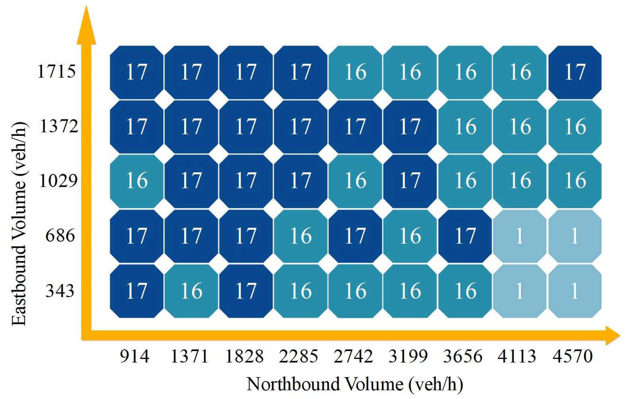
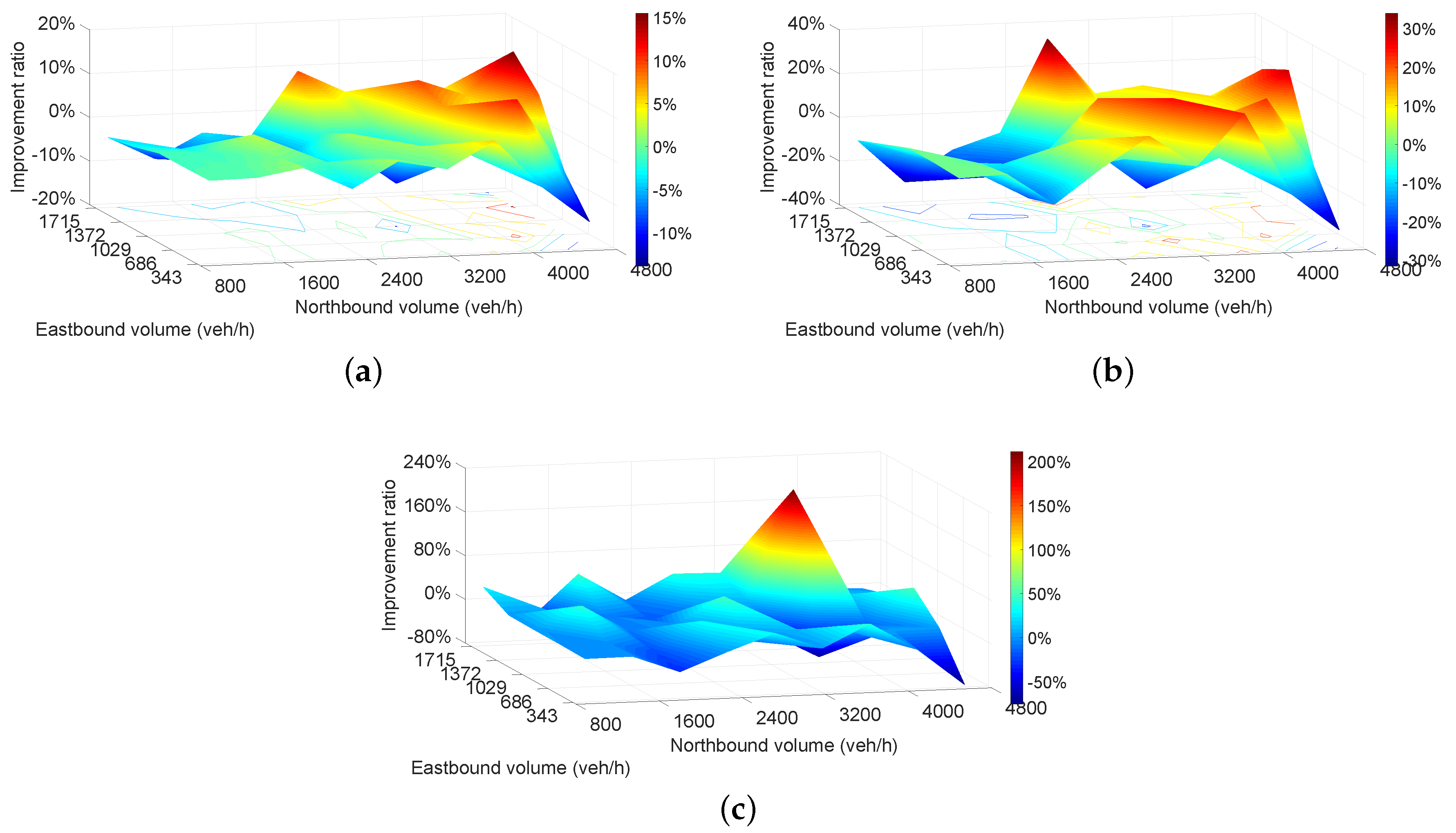
4.4. Sensitivity Analysis of Operational Performance

Scheme 17 performs better than Scheme 16, but

Table 4. VISSIM results of three selected schemes with evening peak hour data.

Item	Travel Time		Delay		Number of Stops
Number 1	695.83		250.64		21.38
Number 16	511.23	−26.53%	181.62	−27.54%	10.0	−53.23%
Number 17	491.51	−29.36%	160.88	−36.22%	7.35	−65.62%

The results of all six flows were summed, and the change rate was compared between Schemes 1 and 16 and Schemes 1 and 17. It can be seen that Scheme 17 is a little bit better than Scheme 16.

only covers investigated data. In order to cover all operating conditions, all different volume combinations should also be simulated and then be compared. The vehicle composition, turning ratio, and expected speed were the same in all simulations. The South–North direction has four lanes, and the maximum volume is 4570 veh/h, while the North–South direction has three lanes, and the maximum volume is 3430 veh/h according to [74] under service level E. The traffic volume changes within 0.2∼1.0 V/C. The West–East direction has three lanes, and the evening peak hour volume is 651 veh/h, while the middle (noon) valley volume is 178 vhe/h: both are far lower than the stipulated content of 3430 veh/h in [74]. For the West–East direction, 0.025∼0.3 V/C was selected. All volume parameters in VISSIM are shown in

Table 5. VISSIM volume in sensitivity analysis.

Item	Value
Southbound volume (veh/h)	686/1029/1372/1715/2058/2401/2744/3087/3430
Northbound volume (veh/h)	914/1371/1828/2285/2742/3199/3656/4113/4570
Eastbound volume (veh/h)	86/172/343/686/1029

Northbound and Southbound changes together as a group, and the whole sensitivity analysis includes the results of 45 simulations in total.

. Traffic light cycles were calculated by Synchro7 for different volume combinations.

The sensitivity analysis can reflect the improvement ratio of Scheme 16 to Scheme 1 and Scheme 17 to Scheme 1. Travel time, delay, and the number of stops are still the three indexes that comprise the sensitivity analysis. The result of Scheme 16 to Scheme 1 is shown in Figure 10:

Figure 10 shows the result for the improvement degree of Scheme 16 to Scheme 1. The improvement ratio is calculated by Ratio = (Scheme 16 − Scheme 1)/Scheme 1 * 100%. Figure 10a shows a significant reduction in travel time compared with Scheme 1. The travel time is reduced by 20∼44% of the whole range. Figure 10b shows the delay change result, and the delay changes depend on the volume combinations. The majority of the delay is reduced by 10∼66%. However, the delay increases in five situations, increasing by as much as 22% when the Northbound volume is under 1828 veh/h. Figure 10c shows the improvement in the number of stops. Besides the five situations in which it increases, the majority of the number of stops is reduced from 10% to 92%. The five increased situations are 30.5%, 56.5%, 71.4%, 110.9%, and 232.7%, respectively, and they are all centralized in the same area as that in the previous two figures.

For all ranges, the change in traffic volume has little influence on the performance of the improvement. The performance of the improvement is relatively uniform for the entire range in Figure 10. When the arterial volume is less than 1371 veh/h or more than 3656 veh/h, the improvement is small, or even deteriorates. The improvement from Scheme 16 has a significant effect on the other parts. When both volumes of two roads are small, Scheme 16 has no improvement effect. The improvement from Scheme 16 shows if the volume increases in either direction. Overall, the improvement of Scheme 16 is clear.

Figure 11 shows the result of Scheme 17 to Scheme 1. Figure 11a shows the change in travel time. Travel time is reduced by 16∼36%, which is a significant improvement. Figure 11b shows the improvement in the delay. The majority is reduced by 10∼66%, while two situations become worse than before, and they are all centralized in the same area as in Figure 10. Figure 11c shows the improvement in the number of stops, and the improvement ratio ranges from 30∼92%, except for two increases.

The impact of volume has a similar trend to that in Figure 10. The improvement decreases when the arterial volume is less than 1371 veh/h or more than 3656 veh/h. Generally, Scheme 17 improves the operation significantly under the majority of conditions.

5. Results

5.1. Weight of Three Indexes

Figure 10 and Figure 11 both show improvement compared with Scheme 1, but no single scheme performs better than the other two schemes under all circumstances. This means that every scheme has its own advantage in different situations. The simulation results are represented with three indexes in the last section, but comparison among schemes with a single standard that includes the weights for the three indexes is needed. The calculation is as follows:

$$T_{jj}=\sum _{i=1}^{45}{T}_j\left(i\right),D_{jj}=\sum _{i=1}^{45}{D}_j\left(i\right),S_{jj}=\sum _{i=1}^{45}{S}_j\left(i\right),\forall j=1,2,3,$$

(6)

where T, D, and S denote travel time, delay, and number of stops, respectively. $i=45$ indicates 45 simulation results for each scheme. $j=1,2,3$ denotes Schemes 1, 16, and 17, respectively. First, the same index of the three schemes needs to be converted into one matrix. In the following steps, T is used as an example.

All 45*3 travel time results have been put into one matrix, named T:

$$T=\left[\begin{array}{ccc}{T}_1\left(1\right)& T_2\left(1\right)& T_3\left(1\right)\\ T_1\left(2\right)& T_2\left(2\right)& T_3\left(2\right)\\ ⋮& ⋮& ⋮\\ T_1\left(45\right)& T_2\left(45\right)& T_3\left(45\right)\end{array}\right].$$

(7)

The other two indexes undergo the same process:

$$\left\{\begin{array}{c}T=[T_1,T_2,T_3],\hfill \\ D=[D_1,D_2,D_3],\hfill \\ S=[S_1,S_2,S_3],\hfill \end{array}\right.$$

(8)

Second, in the T matrix, the minimum value of each row is selected, and then the minimum value and its corresponding column number are the output. The 45 minimum values represent the minimum travel time in 45 simulations. A new matrix is generated, named $T_m$.

$$T_m\left(i\right)=\left[\begin{array}{c}minT(1,j)\\ minT(2,j)\\ ⋮\\ minT(45,j)\end{array}\right],j=1:3.$$

(9)

All three matrices of Equation (8) can be calculated as

$$\left\{\begin{array}{c}{T}_m\left(i\right)=minT(i,j),\hfill \\ D_m\left(i\right)=minD(i,j),\hfill \\ S_m\left(i\right)=minS(i,j),\hfill & \hfill i=1:45,j=1:3;\end{array}\right.$$

(10)

where $T_m$ is a matrix that contains the minimum travel time value of each volume combination.

Third, the weights of the three indexes are calculated, and the three indexes are put into one single matrix, Y:

$$Y=\left[\begin{array}{ccc}{T}_m(1,j)& D_m(1,j)& S_m(1,j)\\ T_m(2,j)& D_m(2,j)& S_m(2,j)\\ ⋮& ⋮& ⋮\\ T_m(45,j)& D_m(45,j)& S_m(45,j)\end{array}\right],j=1:3.$$

(11)

To rank the different schemes, it is necessary to rate the simulation result of each traffic condition. The scoring is based on the calculation of the respective weights of the three indexes, namely, travel time, delay, and the number of stops. The entropy method is a common weighting method used to measure value dispersion in decision-making, with regard to the more dispersed, the more differentiated, and the ones with more information. At the same time, indexes should be given higher weight, and vice versa. The entropy method was used to calculate the weights of the three indexes objectively, instead of using artificial weights. In Equation (11), the greater gap between index $y\left(ij\right)$ means that $y\left(j\right)$ has a greater role. If an index value is the same as another, that means that there is no effect on the final evaluation.

All values should be standardized before the next calculation step since the various indexes are not uniform. Absolute values are converted into relative values, $y_{ij}=\left|y_{ij}\right|$, to solve the problem of homogenization of different qualitative indicators. The calculation is given below:

$$y_{ij}=\frac{y_{ij}-min\{y_{ij},\dots ,y_{nj}\}}{max\{x_{1j},\dots ,x_{nj}\}-min\{x_{1j},\dots ,x_{nj}\}}.$$

(12)

The weight of index j of scheme i is calculated as follows:

$$p_{ij}=\frac{y_{ij}}{{\displaystyle \sum _{i=1}^3}{y}_{ij}},i=1:45,j=1:3.$$

(13)

The entropy value of index j is calculated as follows:

$$e_j=-k\sum _{i=1}^n{p}_{ij}ln\left(p_{ij}\right),$$

(14)

where $k=1/ln\left(n\right)$ and satisfies $e_j\ge 0$.

The entropy redundancy is calculated as follows:

$$d_j=1-e_j.$$

(15)

The weight of each index is calculated as follows:

$$p_{ij}=\frac{d_j}{{\displaystyle \sum _{j=1}^3}{d}_j}.$$

(16)

The weight calculation results are shown in

Table 6. Weights of three indexes.

Index	T	D	S	Summation
Weight	0.2100	0.3873	0.4027	1.0000

:

5.2. Schemes Comparison

The corresponding number is chosen from matrix Y to generate a new matrix $A=zeros(45\times 3)$, as follows:

$$\sum _{i=1}^{45}\sum _{j=1}^{3}A=\left\{\begin{array}{cc}A(i,1)=w\left(j\right)\hfill & \mathrm{if}Y(i,j)=1\hfill \\ A(i,2)=w\left(j\right)\hfill & \mathrm{if}Y(i,j)=2\hfill \\ A(i,3)=w\left(j\right)\hfill & \mathrm{if}Y(i,j)=3\hfill \end{array}\right.$$

(17)

where $w\left(j\right),j=1:3$ denotes the weight in Table 6. Each row of Y (Equation (11)) has three numbers for three indexes, and each number is the best scheme calculated. For example, the first row in matrix Y is

$$Y[1,.]=\left[332\right].$$

(18)

Equation (18) indicates that Scheme 17 performs better than Scheme 16 and Scheme 1 under the conditions in the first row in matrix Y. The weight of Scheme 17 in $Y[1,.]$ is

$$w\left(2\right)=0+0+0.4027=0.4027.$$

(19)

$$w\left(3\right)=0.2100+0.3873+0=0.5973.$$

(20)

Thus, the first row of matrix A is

$$A[1,.]=\left[001\right].$$

(21)

The columns in matrix A represent Schemes 1, 16, and 17, respectively. The result in the first row is Scheme 17 in matrix A, according to Equation (21). After repeating Equations (17)∼(21), the final matrix T can be generated with the final result:

$$T(i)=\left\{maxA[i,.]\right\}\left(j\right).$$

(22)

Matrix T contains 45 scheme numbers that represent the best scheme under each condition. Matrix T is transposed into a $9\times 5$ matrix, and the final result is plotted in Figure 12:

Figure 12 shows the comparison matrix of the three schemes with all 45 volume combinations. Scheme 1 only appears in the corner of the matrix. The two conditions in which Scheme 1 is the best are an Eastbound volume of 86 veh/h and a Northbound volume of 1371 veh/h. Considering the delay and number of stops, Schemes 16 and 17 perform worse, but they perform better if travel time is the only standard.

Scheme 17 shows the best performance 24 times among the 45 situations. Scheme 17 is better than the other two schemes when the flow increases in all directions. As the Eastbound volume increases, Scheme 17 performs increasingly better. The effects of Scheme 16 are the opposite of Scheme 17 results: Scheme 16 is better as the Eastbound volume decreases. The best performance of Scheme 16 and 17 is 19:24.

When the Northbound volume range is 914∼1828 veh/h, Scheme 17 performs much better than Scheme 16; the ratio of the two schemes is 11:2. When the Northbound volume increases from 2285 to 3199 veh/h, Scheme 16 becomes much better than the other two schemes: Scheme 16 occupies 9 blocks, while Scheme 17 only occupies 6 blocks. If the Northbound volume is more than 3656 veh/h, the result of Scheme 17 is similar to that of Scheme 16, and the ratio is 8:7.

The Eastbound volume variation has some influence on the result. When the Eastbound volume is 86 veh/h, Scheme 16 performs much better than Scheme 17. When the Eastbound volume ranges from 172 to 686 veh/h, Scheme 16 performs similarly to Scheme 17. When the Eastbound volume is 1029 veh/h, Scheme 17 shows a great advantage relative to Scheme 16.

Although Figure 12 indicates the better performance of Schemes 16 and 17, for real traffic management, only one scheme can be used in practice. Both Schemes 16 and 17 are good, but the difference between the two schemes still needs to be calculated. The ratio of improvement from Scheme 17 to Scheme 16 is calculated as Ratio = (Scheme 17 − Scheme 16)/Scheme 16 * 100%. The result is shown in Figure 13:

Figure 13 shows the difference between Schemes 16 and 17. For travel time, the two schemes have 22% error at most. For delay, the two schemes have 44% at most, whereas the difference for the number of stops is 236%. The errors between the two schemes are pronounced, and this means that different volumes require different corresponding schemes. The result in Figure 13 supports the validity of the result in Figure 12. Scheme 17 occupies more blocks than Scheme 16 in Figure 12. In Figure 13, with evening peak-hour data, Scheme 17 also performs better than Scheme 16 when the volumes are the same.

For safety performance, the result of Table 3, the safety evaluation showed the great improvement of Schemes 16 and 17 to Scheme 1. Schemes 16 and 17 drastically reduced or eliminated instances of crossing from 362 to 1 and 0. Rear ends were reduced from 609 to 207 and 169, with 66% and 78% improvement, respectively. The lane changes were reduced from 102 to 62 and 64, which is also a significant improvement. Scheme 17 performed better on all three indexes compared to Scheme 16 and 1, which also indicates that Scheme 17 is better than Scheme 16 and 1. Above all, Scheme 17 is a better improvement scheme for this non-aligned intersection caused by a work zone.

6. Conclusions

Sustainable urban transportation is one of many major issues in urban development in the world today. The impact of work zones throughout the city on sustainable traffic flow is enormous. China is still in a rapid urban construction period, with a rapid increase in private vehicles and the urban population. The traffic system is fragile, but construction is inevitable. Road reconstruction, urban pipeline construction, and subway construction are distributed throughout Chinese cities. At first, a work zone could take up as much land as needed, but soon, people found that an extensive work zone area had a serious impact on traffic operation. Therefore, the occupation area of work zones in cities was reduced as much as possible in recent years in an attempt to reduce the impact on traffic. However, construction periods can last from several months to several years. In some cases, the work zone area is still very large, such as subway work zones. Trying to reduce the work zone area and road encroachment without a specific study on the affected traffic cannot eliminate these very serious traffic problems.

The intersection studied in this article has been shown in Figure 3. The roads on both sides of the intersection are only four lanes wide, while the intersection is as wide as 11 lanes. The wider the road, the larger the traffic capacity, and ignoring the traffic bottleneck caused by merging in a short segment is not appropriate. Sustainable traffic flow will be interrupted in the bottleneck section.

This paper proposes two traffic improvement measures for urban intersections occupied by work zones. Both measures are based on the same core content, namely, the channelization of sustainable traffic flow. The chaos of vehicles when passing through the intersections stems from the fact that there are no lane lines in the intersection area, and there is no horizontal restriction of traffic flow either. A large number of merge movements causes congestion, delay, and stops after passing through the intersection, and it increases accident risks and safety hazards. By adding railing to limit the width of traffic flow and maintaining the same width of the road on both sides of the intersection, traffic problems can be greatly reduced, while also providing a larger area for the work zone.

Of the two improvements proposed in this paper, one (Scheme 16) is the addition of railing to limit the width of traffic flow in the present situation, while the other one (Scheme 17) is a better situation from the perspective of a feasible work zone layout. The traffic flow remains straight when passing through the intersection area as though passing through a normal intersection. After passing through the intersection, the direction changes as the road turns.

The other schemes in Table 3 were used to explore whether the road offset value had a significant relationship with traffic operation under the control of the width of traffic flow. The results show that the relationship is not strong. Furthermore, in practice, the offset of road misalignment is not actively chosen by people, but is determined by the limitations of the work zone. Only Schemes 16 and 17 are feasible and have minimal impact on the work zone layout.

In this research, we proposed two schemes, two ways of channelization, to reduce the unsustainable traffic caused by work zone at intersections. Real traffic data were collected and input into VISSIM to simulate and evaluate the different schemes. Through the research, no obvious relationship was found to exist with offset values at the non-aligned intersection. The travel time, delay, and number of stops were the three indexes of evaluation. The entropy method was used to calculate the weight of three indexes, which determined the schemes selection matrix in the end. The selection matrix can be used for scheme selection for different combinations. Scheme 17 performed the best according to the traffic volumes collected.

The research in this paper can be applied to evaluate the impact of a work zone on urban sustainable traffic flow. Using two corresponding improvement schemes can greatly alleviate congestion, reduce travel time, delay, and the number of stops. The core of the improvement is the channelized management of sustainable traffic flow. For the roads occupied by the work area, the results of this study can greatly reduce the impact on traffic. Compared with a state without any control measures, the travel time can be reduced by up to 44%, delays can be reduced by up to 66%, and parking times can be reduced by up to 92%. There are still some topics in this article that can be studied further—the first is how to improve the traffic operation situation caused by the working area at the intersection, while the second is the impact of the advanced parking line in Scheme 17 on traffic operations.

References

1. Xue, Y.; Cao, X.; Ai, Y.; Xu, K.; Zhang, Y. Primary Air Pollutants Emissions Variation Characteristics and Future Control Strategies for Transportation Sector in Beijing, China. Sustainability 2020, 12, 4111. [Google Scholar] [CrossRef]
2. Wang, J.; Lu, H.; Sun, Z.; Wang, T.; Wang, K. Investigating the Impact of Various Risk Factors on Victims of Traffic Accidents. Sustainability 2020, 12, 3934. [Google Scholar] [CrossRef]
3. Baghestani, A.; Tayarani, M.; Allahviranloo, M.; Gao, H.O. Evaluating the Traffic and Emissions Impacts of Congestion Pricing in New York City. Sustainability 2020, 12, 3655. [Google Scholar] [CrossRef]
4. Leong, L.V.; Vivian, W.W.L.; Wins, C.G. Effects of Short Exit Lane on Gap-Acceptance and Merging Behavior of Drivers Turning Right at Unconventional T-Junctions. Int. J. Civ. Eng. 2020, 18, 19–36. [Google Scholar] [CrossRef]
5. Zlatkovic, M.; Zlatkovic, S.; Sullivan, T.; Bjornstad, J.; Shahandashti, S.K. Assessment of effects of street connectivity on traffic performance and sustainability within communities and neighborhoods through-traffic simulation. Sustain. Cities Soc. 2019, 46, 101409. [Google Scholar] [CrossRef]
6. Hamurcu, M.; Eren, T. Strategic planning Based on Sustainability for Urban Transportation: An Application to Decision-Making. Sustainability 2020, 12, 3589. [Google Scholar] [CrossRef]
7. Cai, Q.; Mohamed, A.A.; Jaeyoung, L.; Wang, L.; Wang, X.S. Developing a grouped random parameters multivariate spatial model to explore zonal effects for segment and intersection crash modeling. Anal. Methods Accid. Res. 2018, 19, 1–15. [Google Scholar] [CrossRef]
8. Echab, H.; Lahouari, N.; Ez-Zahraouy, H.; Benyoussef, A. Phase diagram of a non-signalized T-shaped intersection. Phys. A Stat. Mech. Appl. 2016, 461, 674–682. [Google Scholar] [CrossRef]
9. Zhang, W.; Kronprasert, N.; Gustafson, J. Unclog Local Network Congestion Using High Capacity Mini-Roundabout: A Feasibility Study. In Proceedings of the Transportation Research Board Meeting, Washington, DC, USA, 12–16 January 2014. [Google Scholar]
10. Mohamed, A.I.Z.; Ci, Y.S.; Tan, Y.Q. A Novel Methodology for Estimating the Capacity and Level of Service for the New Mega Elliptical Roundabout Intersection. J. Adv. Transp. 2020, 2020, 8467152. [Google Scholar] [CrossRef] [Green Version]
11. Jaepil, M.; Kim, Y.; Kim, D.; Lee, S. The potential to implement a superstreet as an unconventional arterial intersection design in Korea. Ksce J. Civ. Eng. 2011, 15, 1109–1114. [Google Scholar]
12. Wonho, S.; Michael, H. Signal design for displaced left-turn intersection using Monte Carlo method. KSCE J. Civ. Eng. 2014, 18, 1140–1149. [Google Scholar]
13. Zhao, J.; Ma, W.J.; Zhang, H.M.; Yang, X.G. Increasing the Capacity of Signalized Intersections with Dynamic Use of Exit Lanes for Left-Turn Traffic. Transp. Res. Rec. 2013, 2355, 49–59. [Google Scholar] [CrossRef]
14. Tang, T.Q.; Zhang, J.; Liu, K. A speed guidance model accounting for the driver’s bounded rationality at a signalized intersection. Phys. A Stat. Mech. Appl. 2017, 473, 45–52. [Google Scholar] [CrossRef]
15. Jenelius, E.; Haris, N.K. Travel time estimation for urban road networks using low frequency probe vehicle data. Transp. Res. Part B Methodol. 2013, 53, 64–81. [Google Scholar] [CrossRef] [Green Version]
16. Shao, Y.; Han, X.Y.; Wu, H.; Claudel, C.G. Evaluating Signalization and Channelization Selections at Intersections Based on an Entropy Method. Entropy 2019, 21, 808. [Google Scholar] [CrossRef] [Green Version]
17. Shao, Y.; Han, X.Y.; Wu, H.; Shan, H.M.; Yang, S.W.; Claudel, C.G. Evaluating the sustainable traffic flow operational features of an exclusive spur dike U-turn lane design. PLoS ONE 2019, 14, e0214759. [Google Scholar] [CrossRef]
18. Mahmoud, T.; Akmal, S.A. Impact of using indirect left-turns on signalized intersections’ performance. Can. J. Civ. Eng. 2017, 44, 462–471. [Google Scholar]
19. Sun, W.L.; Wu, X.K.; Wang, Y.P.; Yu, G.Z. A continuous-flow-intersection-lite design and traffic control for oversaturated bottleneck intersections. Transp. Res. Part C Emerg. Technol. 2015, 56, 18–33. [Google Scholar] [CrossRef]
20. Narayana, R.; Shriniwas, S.A.; Gaurang, J. Effect of Construction Work Zone on Traffic Stream Parameters Using Vehicular Trajectory Data under Mixed Traffic Conditions. J. Transp. Eng. Part A Syst. 2020, 146, 05020002. [Google Scholar]
21. Didier, V.; Carla, L.D.P.; Benjamin, C.; Alberto, F.; Ricardo, G.R.; Enid, C.T.; Maria, X.R.I. Comparative Analysis between Distracted Driving Texting Laws and Driver’s Behavior in Construction Work Zones. J. Leg. Aff. Disput. Resolut. Eng. Constr. 2019, 11, 04519026. [Google Scholar]
22. Lu, C.; Dong, J.; Sharma, A.; Huang, T.; Knickerbocker, S. Predicting Freeway Work Zone Capacity Distribution Based on Logistic Speed-Density Models. J. Adv. Transp. 2018, 2018. [Google Scholar] [CrossRef]
23. Bing, Z.; Bingjie, Z. Evaluation of Traffic Organization Scheme during the Construction of Urban Subway Station based on TransCAD. Appl. Mech. Mater. 2014, 505–506, 433–436. [Google Scholar]
24. Huang, Y.; Bai, Y. Driver responses to graphic-aided portable changeable message signs in highway work zones. J. Transp. Saf. Secur. 2019, 11, 661–682. [Google Scholar] [CrossRef]
25. Nawaf, M.A.; Elena, P. Impact Assessment of Short-Term Work Zones on Intersection Capacity in New York City. Transp. Res. Rec. 2018, 2672, 1–8. [Google Scholar]
26. Zhang, K.; Hassan, M. Crash severity analysis of nighttime and daytime highway work zone crashes. PLoS ONE 2019, 14, e0221128. [Google Scholar] [CrossRef] [PubMed] [Green Version]
27. Pesti, G.; Chu, C.L.; Balke, K.; Shelton, J.; Zeng, X.; Chaudhary, N. Regional Impact of Roadway Construction on Traffic Operations. Transp. Res. Rec. 2012, 2272, 56–66. [Google Scholar] [CrossRef]
28. Zhang, C.; Qin, J.; Zhang, M.; Zhang, H.; Hou, Y. Practical Road-Resistance Functions for Expressway Work Zones in Occupied Lane Conditions. Sustainability 2019, 11, 382. [Google Scholar] [CrossRef] [Green Version]
29. Bharadwaj, N.; Edara, P.; Sun, C.; Brown, H.; Chang, Y. Traffic Flow Modeling of Diverse Work Zone Activities. Transp. Res. Rec. 2018, 2672, 23–34. [Google Scholar] [CrossRef] [Green Version]
30. Arezoo, M.; Jay, M.R.; Stephen, P.M.; James, C.W.; Hossein, H. An optimization based traffic diversion model during construction closures. Comput. Aided Civ. Infrastruct. Eng. 2019, 34, 1087–1099. [Google Scholar]
31. Fei, L.; Zhu, H.B.; Han, X.L. Analysis of traffic congestion induced by the work zone. Phys. A Stat. Mech. Appl. 2016, 450, 497–505. [Google Scholar] [CrossRef]
32. Yun, Y.; Yue, L.; Weiyan, L. Dynamic Lane-Based Signal Merge Control for Freeway Work Zone Operations. J. Transp. Eng. Part A Syst. 2019, 145, 04019053. [Google Scholar] [CrossRef]
33. Schroeder, B.J.; Nagui, M. Rouphail. Estimating Operational Impacts of Freeway Work Zones on Extended Facilities. Transp. Res. Rec. 2010, 2169, 70–80. [Google Scholar] [CrossRef]
34. Zheng, H.; Sun, Z.; Chen, X. Evaluation on Traffic Guidance Plan during Construction Period based on Vissim Simulation. In Proceedings of the 2017 International Conference on Computer Network, Electronic and Automation, Xi’an, China, 23–25 September 2017. [Google Scholar]
35. Huaizhong, Z.; Shunying, Z.; Yu, W.; Shuang, D. Evaluation of Traffic Organization Scheme during Highway Reconstruction Period. Appl. Mech. Mater. 2013, 361–363, 2007–2011. [Google Scholar]
36. Sze-Chum, L.; Ming, L.; Chi-Sun, P. Integration of construction and traffic engineering in simulating pipe-jacking operations in urban areas. In Proceedings of the 2011 Winter Simulation Conference, Phoenix, AZ, USA, 11–14 December 2011. [Google Scholar]
37. Ravi, B.; Sewa, R.; Kayitha, R. Impact of metro rail construction work zone on traffic environment. In Proceedings of the 11th Transportation Planning and Implementation Methodologies for Developing Countries (TPMDC), Mumbai, India, 10–12 December 2014. [Google Scholar]
38. Chen, X.; Lu, J.; Zhao, J.; Qu, Z.; Yang, Y.; Xian, J. Traffic Flow Prediction at Varied Time Scales via Ensemble Empirical Mode Decomposition and Artificial Neural Network. Sustainability 2020, 12, 3678. [Google Scholar] [CrossRef]
39. Song, Y.; Zlatkovic, M.; Richard, J.P. Evaluation of GPS-Based Transit Signal Priority for Mixed-Traffic Bus Rapid Transit. Transp. Res. Rec. 2016, 2539, 30–39. [Google Scholar] [CrossRef]
40. Stevanovic, A.; Dakic, I.; Zlatkovic, M. Comparison of adaptive traffic control benefits for recurring and non-recurring traffic conditions. IET Intell. Transp. Syst. 2017, 11, 142–151. [Google Scholar] [CrossRef]
41. Kurt, D.; Peter, S. A multiagent approach to autonomous intersection management. J. Artif. Intell. Res. 2008, 31, 591–656. [Google Scholar]
42. Stuart, T.G.; Thomas, J.T.; Brian, N.F. Driving simulator validation for speed research. Accid. Anal. Prev. 2002, 34, 589–600. [Google Scholar]
43. Du, B.; Chien, S.; Lee, J.; Lazar, S.; Kyriacos, M. Artificial Neural Network Model for Estimating Temporal and Spatial Freeway Work Zone Delay Using Probe-Vehicle Data. Transp. Res. Rec. 2016, 2573, 164–171. [Google Scholar] [CrossRef]
44. Harith, A.; Alireza, M.; Mohammad, R.K.S.; Haizhong, W. Measuring the impacts of connected vehicles on travel time reliability in a work zone environment: An agent-based approach. J. Intell. Transp. Syst. 2019. [Google Scholar] [CrossRef]
45. Kim, K.J.; Kim, K. Case Study on the Evaluation of Equipment Flow at a work zone. J. Comput. Civ. Eng. 2010, 24, 570–575. [Google Scholar] [CrossRef]
46. Zlatkovic, M.; Porter, R.J.; Kergaye, C. Performance-Based Warranty Contracts for Pavement Markings: Experience and Lessons Learned in the State of Utah. Transp. Res. Rec. 2015, 2504, 49–57. [Google Scholar] [CrossRef]
47. Zhao, J.; Ma, W.; Head, K.L.; Yang, X.G. Optimal operation of displaced left-turn intersections: A lane-based approach. Transp. Res. Part C Emerg. Technol. 2015, 61, 29–48. [Google Scholar] [CrossRef]
48. Do, G.K.; Simon, W. The significance of endogeneity problems in crash models: An examination of left-turn lanes in intersection crash models. Accid. Anal. Prev. 2006, 38, 1094–1100. [Google Scholar]
49. Ma, W.J.; Liu, Y.; Zhao, J.; Wu, N. Increasing the capacity of signalized intersections with left-turn waiting areas. Transp. Res. Part A 2017, 105, 181–196. [Google Scholar] [CrossRef]
50. Xuan, Y.G.; Carlos, F.D.; Michael, J.C. Increasing the capacity of signalized intersections with separate left turn phases. Transp. Res. Part B 2011, 45, 769–781. [Google Scholar] [CrossRef]
51. Dakic, I.; Mladenovic, M.N.; Stevanovic, A.; Zlatkovic, M. Upgrade Evaluation of Traffic Signal Assets: High-resolution Performance Measurement Framework. Promet-Traffic Transp. 2018, 30, 323–332. [Google Scholar] [CrossRef]
52. Zlatkovic, M.; Stevanovic, A.; Peter, T.M. Development and Evaluation of Algorithm for Resolution of Conflicting Transit Signal Priority Requests. Transp. Res. Rec. 2012, 2311, 167–175. [Google Scholar] [CrossRef]
53. Juraek, O.; Eungcheol, K.; Myungseob, K.; Sangho, C. Development of conflict techniques for left-turn and cross-traffic at protected left-turn signalized intersections. Saf. Sci. 2010, 48, 460–468. [Google Scholar]
54. Nikiforos, S.; Adam, H.; Adam, K. A simulation-based approach in determining permitted left-turn capacities. Transp. Res. Part C Emerg. Technol. 2015, 55, 486–495. [Google Scholar]
55. Wu, J.M.; Liu, P.; Tian, Z.Z.; Xu, C.C. Operational analysis of the contraflow left-turn lane design at signalized intersections in China. Transp. Res. Part C Emerg. Technol. 2016, 69, 228–241. [Google Scholar] [CrossRef]
56. Ma, C.X.; Hao, W.; Wang, A.B.; Zhao, H.X. Developing a Coordinated Signal Control System for Urban Ring Road under the Vehicle-infrastructure Connected Environment. IEEE Access 2018, 6, 52471–52478. [Google Scholar] [CrossRef]
57. Yan, X.D.; Essam, R.; Guo, D.H. Effects of major-road vehicle speed and driver age and gender on left-turn gap acceptance. Accid. Anal. Prev. 2007, 39, 843–852. [Google Scholar] [CrossRef] [PubMed]
58. Shaaban, K.; Hamad, H. Critical Gap Comparison between One-, Two-, and Three-Lane Roundabouts in Qatar. Sustainability 2020, 12, 4232. [Google Scholar] [CrossRef]
59. Xi’an Municipal Bureau of Statistics. 2019 Xi’an Statistical Yearbook; China Statistics Press: Beijing, China, 2019. Available online: http://tjj.xa.gov.cn/tjnj/2019/zk/indexeh.htm (accessed on 10 May 2020).
60. Xi’an Goveronment Homepage. Profile of Xi’an. 2020. Available online: http://en.xa.gov.cn/thisisxian/profile/944.htm (accessed on 10 May 2020).
61. Zhang, J.; Wang, Y.Q.; Zhou, W. Research on relic protection in Xi’an subway engineering. In Proceedings of the 2011 International Symposium on Water Resource and Environmental Protection (ISWREP 2011), Xi’an, China, 20–22 May 2011. [Google Scholar] [CrossRef]
62. AutoNavi Traffic Big-Data. 2019. Traffic Analysis Reports for Major Cities in China. 2020. Available online: Https://report.amap.com/share.do?id=8b04ff737067a78601707b2ba0542d72 (accessed on 25 February 2020).
63. Zhao, Y.; Liu, P.; Chen, Y.G.; Hao, Y. Can Left-turn Waiting Areas Improve the Capacity of Left-turn Lanes at Signalized Intersections? Procedia-Soc. Behav. Sci. 2012, 43, 192–200. [Google Scholar]
64. Ronald, T.M.; Fred, C. Recommended guidelines for the calibration and validation of traffic simulation models. In Proceedings of the 8th TRB Conference on the Application of Transportation Schemening Methods, Corpus Christi, TX, USA, 22–26 April 2002; pp. 178–187. [Google Scholar]
65. Park, B.; Won, J.; Yun, I. Application of Microscopic Simulation Model Calibration and Validation Procedure: Case Study of Coordinated Actuated Signal System. Transp. Res. Rec. 2006, 1978, 113–122. [Google Scholar] [CrossRef]
66. Chu, L.Y.; Liu, H.; Oh, J.S.; Recker, W. A calibration procedure for microscopic traffic simulation. In Proceedings of the Intelligent Transportation Systems, Shanghai, China, 12–15 October 2003; Volume 2, pp. 1574–1579. [Google Scholar]
67. Xiang, Y.; Li, Z.; Wang, W.; Chen, J.; Wang, H.; Li, Y. Evaluating the Operational Features of an Unconventional Dual-Bay U-Turn Design for Intersections. PLoS ONE 2016, 11, e0163758. [Google Scholar] [CrossRef] [Green Version]
68. Sun, J. Guideline for Microscopic Traffic Simulation Analysis; Tongji University Press: Shanghai, China, 2014. [Google Scholar]
69. Jayasooriya, N.; Bandara, S. Calibrating and validating VISSIM microscopic simulation software for the context of Sri Lanka. In Proceedings of the 2018 Moratuwa Engineering Research Conference (MERCon), Moratuwa, Sri Lanka, 30 May–1 June 2018; pp. 494–499. [Google Scholar]
70. Henclewood, D.; Suh, W.; Rodgers, M.O.; Fujimoto, R.; Hunter, M.P. A calibration procedure for increasing the accuracy of microscopic traffic simulation models. Simulation 2017, 93, 35–47. [Google Scholar] [CrossRef]
71. Federal Highway Administration Research and Technology. Surrogate Safety Assessment Model (SSAM) Publications. 2017. Available online: https://www.fhwa.dot.gov/publications/lists/020.cfm (accessed on 10 May 2020).
72. Federal Highway Administration (FHWA). TECHBRIEF Surrogate Safety Assessment Model (SSAM); Federal Highway Administration: Washiton, DC, USA, 2008. [Google Scholar]
73. Federal Highway Administration (FHWA). Surrogate Safety Assessment Model (SSAM)–SOFTWARE USER MANUAL; Federal Highway Administration: Washiton, DC, USA, 2008. [Google Scholar]
74. Transportation Research Board (TRB). Highway Capacity Manual, Sixth Edition: A Guide for Multimodal Mobility Analysis; Transportation Research Board: Washiton, DC, USA, 2016. [Google Scholar]
Figure 1. Dual T-intersection and non-aligned intersection. The dual T-intersection (left) is made up of two adjacent T-intersections and two traffic lights controlled separately, whereas a non-aligned intersection (right) is controlled by a single traffic light, and the through-traffic will be offset when passing the intersection.
Sustainability 12 05494 g001
Figure 2. The investigated intersection location scheme. The investigated intersection is a T-intersection and located in the center of Xi’an CBD district. The arterial street is a North–South seven-lane road, and the collector street is a West–East seven-lane road.
Sustainability 12 05494 g002
Figure 3. The present situation of the T-intersection. This graphic was taken by a drone at a height of 130 m. A construction site occupies the North part of the intersection and forces operating vehicles to be offset by 28 m. Another construction site occupies half of the road area of the southern road of the intersection. Coordinates: 108.889684, 34.205037.
Sustainability 12 05494 g003
Figure 4. The congestion index in Xi’an on 17 January 2019. The real-time congestion index can be gathered from the Autonavi Company Webpage at https://report.amap.com/detail.do?city=610100.
Sustainability 12 05494 g004
Figure 5. The collected trajectories of the intersection. Because of the large area of the intersection, Northbound traffic made up 11 lines of flow at most, and then merged into four lanes. Trajectories of each lane are noted by alphabetic characters A~G, and the number of vehicles from each Northbound lane is also noted. Southbound and Westbound vehicles operated smoothly.
Sustainability 12 05494 g005
Figure 6. The situations of the intersection. (A) Original situation of the intersection. (B) Present situation, work zones occupy part of the area. (C) Improved scheme 1. (D) Improved scheme 2.
Sustainability 12 05494 g006
Figure 7. Simulation schemes. Scheme (C) changes the offset distance to determine the influence of the offset. Scheme (D) is intended to determine another improved scheme with straight length changes.
Sustainability 12 05494 g007
Figure 8. Simulation results of 23 situations with collected data in Table 1. (a) Travel time. (b) Delay. (c) Number of stops. The X-axis shows the 23 simulations; 1 denotes the present situation, 2∼16 denote offset situations, and 17∼23 denote straight length simulations.
Sustainability 12 05494 g008
Figure 9. Overlap of Schemes 16 and 17. The overlap between improved Schemes 16 and 17 shows that these two schemes have the least impact on the work zone. The redesigned route of Scheme 17 occupies a little area (S1) of the work zone and provides a larger area (S2) for the work zone. It is easy to find, regardless of whether the offset value is narrowed or the extension of the straight length occupies a larger area.
Sustainability 12 05494 g009
Figure 10. Improvement ratio of Scheme 16 compared with Scheme 1. (a) Travel time. (b) Delay. (c) Number of stops.
Sustainability 12 05494 g010
Figure 11. Improvement ratio of Scheme 17 compared with Scheme 1. (a) Travel time. (b) Delay. (c) Number of stops.
Sustainability 12 05494 g011
Figure 12. Performances of Schemes 1, 16 and 17. The numbers in the figure represent the scheme number, and the number means the best performance among the three schemes for one volume combination.
Sustainability 12 05494 g012
Figure 13. Improvement ratio of Scheme 17 compared with Scheme 16. (a) Travel time. (b) Delay. (c) Number of stops.
Sustainability 12 05494 g013