Integration of PCA and Fuzzy Clustering for Delineation of Soil Management Zones and Cost-Efficiency Analysis in a Citrus Plantation

Abstract

Citrus spp. are one of the most important commercial crops with global marketing potential in the world, as in Iran. A soil management zone (MZ) as an appropriate approach is necessary to achieve sustainable production, along with improving soil management and increasing economic benefits in the commercial citrus plantations of northern Iran. As the first report, the biological and terrain attributes along with the physicochemical properties (57 soil samples, 0–30 cm) were used for MZ delineation using the integration of principal component analysis (PCA) and the fuzzy c-means clustering methods. An economic analysis based on the MZ results was also performed to determine the changes in each MZ using a relative cost (RC) value. The high correlation between soil properties and terrain attributes and the considerable spatial variation of these factors in the study area call for site-specific nutrient management. The optimal number of MZs was six and there was a significant heterogeneity variation among different MZs. The ranking of the MZs were MZ5 > MZ2 > MZ6 > MZ1 > MZ3 > MZ4 based on higher soil quality and lower costs per tree. The MZ4, MZ3, MZ1, MZ6, and MZ2 required 34.4, 30.6, 29.4, 9.77, and 9.44% more costs than MZ5 (as reference MZ) for achieving similar productivity, respectively. Therefore, this simple and cost-effective approach could be an initial step to utilize fertilizers site-specifically for data-scarce areas and reduce the soil property variability within the delineated MZs, which is fundamental for precision agriculture management.

1. Introduction

Citrus is one of the most important commercial crops with global marketing potential, which is grown across the world, particularly in tropical and subtropical countries [1,2]. It is important due to its role in human diets, as citrus fruits contain a high level of vitamin C and other essential nutrients, such as folate, potassium, and dietary fiber [3]. Annual global production of fresh citrus fruits has been growing in the last several decades, from 30 thousand tons in the 1960s to 130,947 thousand tons in 2015 [4]. Iran, the world’s seventh largest citrus-producing country, followed by Brazil, China, United States, Mexico, India, and Spain, has an annual production of 3739 thousand tons of fresh citrus fruits from an area of ~230,000 ha [4]. The growing demands for crop products in the 21st century have increased the request for new methods to evaluate the soil fertility status in an economical and environmentally friendly manner [5,6]. Moreover, the knowledge of spatial soil fertility status is important to intensive agricultural practices for sustainable agriculture [6,7].

Defining the homogeneous management zones (MZs) is vital for sustainable use of resources and economical aspects for gardeners and farmers [8]. In this regard, the use of soil management zones is necessary to achieve sustainable agriculture and a cost-effective approach for improving the management of citrus plantations.

Considerable advances in statistical techniques and modeling approaches have allowed different agricultural zones to be accurately delineated with new methods like machine learning, GIS, remote sensing, geostatistics, and kriging at a regional and farm scale [5,9]. Several methods and approaches, such as delineating by an active canopy sensor [10], using soil properties by fuzzy k-means cluster analysis [11,12], fuzzy c-means clustering algorithm, principal component analysis (PCA) [12,13,14,15,16,17], and soil fertility analysis [13] have been used to delineate different MZs. However, the selection of the techniques or approaches depends on the purposes of the determination of MZ and the complexity of each approach.

Different types of environmental and soil data could be used for delineating the MZs [10]. For instance, pedo-geomorphological factors [18], soil nutrients [19,20], intrinsic soil properties (e.g., electrical conductivity (EC), pH, particle size distribution, soil organic matter, cation exchange capacity, nitrogen, phosphorous, and potassium) [9,10,12,15,21] can be used for this purpose. Different types of information can be integrated to define MZs by using a clustering algorithm. This effective approach is capable of identifying zones or regions in the fields or farms that internally have similar soil properties, conditions, and productivity potentials [5]. In the application of site-specific management zones, several studies reported successful application of MZ delineation for agricultural purposes, fertilizer application, and farm management [12,22,23]. Aggelopooulou et al. [24], in an apple orchard in Greece, delineated four zones using soil and tree properties, which required different management of irrigation, fertilizer, and cultural activities. In coffee fields, by using physiochemical soil properties and the advantage of geostatistical analysis with fuzzy c-means clustering, Valente et al. [25] reported that it is required to use more than one soil property for better MZ delineation. Furthermore, Peralta et al. [26] delineated MZs in wheat fields in Argentina for the increment of nitrogen efficiency.

In most countries, such as Iran, the fertilizer and nutrient recommendations for agricultural lands are usually uniform on a regional scale [15] or farm scale [10,26], with the spatial heterogeneity of nutrient content in soils being often ignored [9]. However, the source of chemical fertilizers in Iran commonly include nitrogen (urea, 46%), phosphorus (triple superphosphate, 46%), potassium (potassium sulfate, 46%), and also cow manure [27]. Therefore, the similar fertilizer recommendations in the farm or regional scales could lead to over-application of fertilizers in areas with high nutrient levels and vice versa [9,15]. Herein, Peralta et al. [26] concluded that MZ delineation could increase the fertilizer efficiency of nitrogen (or other nutrients) in the commercial fields, and the risk of pollution will decrease along with a decrease in the application of resources, resulting in an increase of economic benefits.

Mazandaran Province, the northern seaside lands of the Caspian Sea, is the main citrus producing area in Iran. The yield of citrus in northern Iran is crucially dependent on soil properties and agricultural practices [27]. Therefore, this study, as the first assessment in a citrus plantation in Iran, aimed to evaluate the potential tools and methods to delineate MZs in the commercial citrus plantations of northern Iran for increasing economic benefits and identifying homogenous zones in this region. The hypothesis for this research is that the MZ could decrease the production costs during the growing season by producing different zones to which to apply various amounts of fertilizers.

2. Materials and Methods

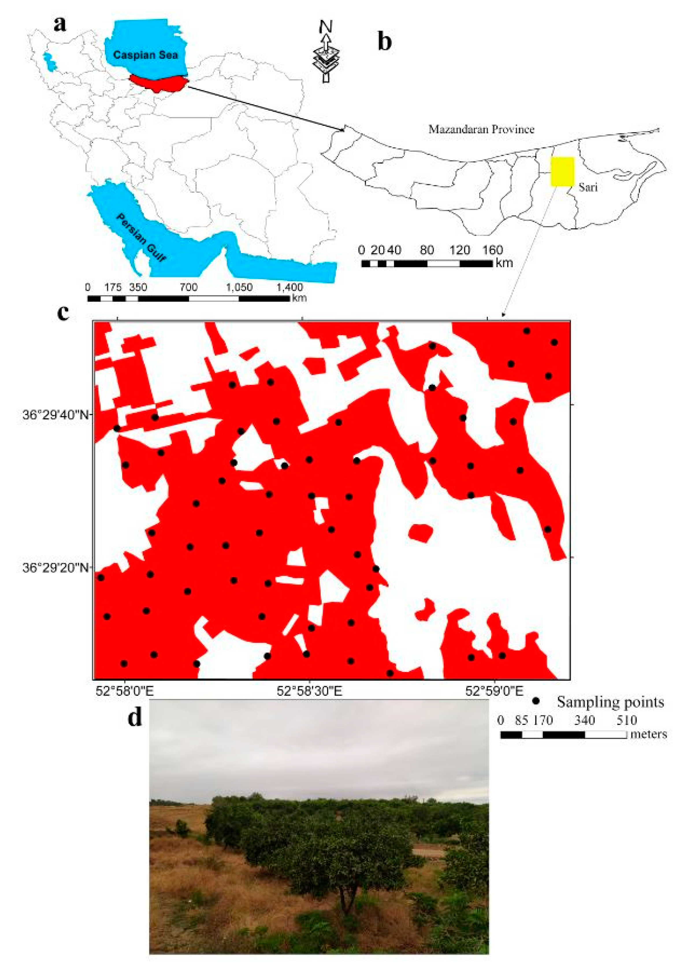
2.1. Study Area

One hundred and sixty hectares of citrus plantation were investigated in northern Iran (Sari region, Mazandaran Province). The study area was located between 52°57′54′′ and 52°59′13′′ E longitudes and 36°29′05′′ and 36°29′50′′ N latitudes, as shown in Figure 1. The mean annual temperature and precipitation were 17.9 °C and 789 mm, respectively. The soil moisture and temperature regime classes are udic and mesic in this region, respectively [28].

2.2. Field Sampling and Data Collection

The soil sampling of MZ delineation tends to decrease the number and cost of the sampling procedure, while it still prepares precise information on soil properties and their spatial variability [29]. Totally, 57 composite soil surface samples (at a depth of 0–30 cm) in the commercial citrus plantation (8–12 year old trees) were taken at randomly chosen sites across the study area, as shown in Figure 1. During soil sampling, we used a portable Global Positioning System (GPS) (Etrex Vista Garmin, Olathe, KS, USA) to accurately mark the sampling points.

2.3. Soil Physicochemical Properties Analysis

The soil samples were air-dried at room temperature (~25 °C), crushed, and passed through a 2 mm sieve for chemical and physical analyses. The wet combustion method [30] was used to determine soil organic carbon (SOC). The soil bulk density (BD) was estimated using the cylindrical core method after 24 h at 105 °C [31]. The soil reaction (pH) [32] and soil electrical conductivity (EC) [33] (both measured on a 1:2.5 suspension) were determined using a multi-parameter apparatus. The Kjeldahl method [34] was used to measure the total nitrogen (TN) of the soil samples. The cation exchange capacity (CEC) was determined using sodium acetate (NaOAc) at a pH of 8.2 [35]. The available soil phosphorus (P_av) [36] and soil available potassium (K_av) [37] were also measured for all soil samples.

Accordingly, 25 g of each air-dried soil sample was placed in a closed glass jar, then moistened (~85% of field capacity) and put in a beaker containing a NaOH (10%) solution therein. The samples were incubated at 30 °C for four days, then the microbial soil respiration (Mres4, mg CO2–C kg⁻¹ soil d⁻¹) was measured using the method suggested by Bakhshandeh et al. [38]. The chloroform fumigation-extraction method was used to determine the microbial carbon biomass (Cmic, mg C kg⁻¹ soil) in the soil samples [39].

2.4. Statistical Analysis

2.4.1. Descriptive Statistics Analysis

The descriptive statistics, including mean, maximum (Max), minimum (Min), median, standard deviation (STD), coefficient of variation (CV), kurtosis coefficients, and skewness, were calculated for all data using the Statistical Analysis System (version 9.4, SAS Institute, Cary, NC, USA, [40]) software. The normality (d) of all soil properties was tested by the Kolmogorov–Smirnov (K–S) test at a significance level of 5%. Based on Warrick and Nielsen [41], the mean values of all attributes around the mean could be classified as data dispersion to three categories as low (CV < 12%), moderate (12 ≤ CV < 60%), and high (CV ≥ 60%).

2.4.2. Spatial Variability Analysis

Considering the sparse sampling points due to the applicability of MZ delineation as an economically and timely approach in the study area, the dataset cannot be directly used for preparing the spatial distribution maps of variables, because many hectares include no data or only a single one, as shown in Figure 1. Although the kriging method is the most common method for interpolation in soil MZ [20,26,42], the semivariograms of the soil variables show a weak to moderate spatial dependence. Therefore, we used the inverse distance weighting (IDW) method to generate the spatial variability maps.

The leave-one-out cross-validation was implemented for testing the performance of the IDW method for predicting the soil and terrain variables in unsampled locations in the study area [43,44]. Three evaluation criteria, including the coefficient of determination (R²), normalized root mean square error (nRMSE, indicating the relative difference (%) of predicted versus observed values), and coefficient of residual mass (CRM) were used for testing the reliability on the interpolation method. The equations of the three evaluation criteria can be written as

$$R^2={\left(\frac{{{\displaystyle \sum }}_{i=1}^n\left(Oi-O\prime \right)\left(Pi-{\rm P}\prime \right)}{\sqrt{{{\displaystyle \sum }}_{i=1}^n{\left(Oi-O\prime \right)}^2}\sqrt{{{\displaystyle \sum }}_{i=1}^n{\left(Pi-P\prime \right)}^2}}\right)}^2$$

(1)

$$nRMSE=\sqrt{\frac{1}{n}{\displaystyle \sum }_{i=1}^n{\left(Pi-Oi\right)}^2}\times \frac{100}{Ň}$$

(2)

$$CRM=1-\frac{{{\displaystyle \sum }}_{i=1}^{n}Oi}{{{\displaystyle \sum }}_{i=1}^{n}O\prime }$$

(3)

where, n is the number of samples, Oi and Pi are the predicted and observed variables, and O′ and P′ are the means for the predicted and observed variables, respectively. Ň is the mean of observed values.

According to Jamieson et al. [45], when the nRMSE is <10%, the results are considered an excellent interpolation; when 10% < nRMSE < 20%, it is a good interpolation; when 20% < nRMSE < 30%, a fair interpolation; and when the nRMSE > 30%, it is considered a poor interpolation. For the CRM criterion, the negative and positive values indicate that the models overestimate and underestimate the observed data, respectively.

2.4.3. Delineation of Management Zone

Briefly, the methodology used for the delineation of MZs consists of the principal component analysis (PCA) on soil and terrain variables and then performing the fuzzy c-means clustering fed with the selected principal components (PCs) to delineate MZs. The PCA, as a dimension reduction approach, uses correlated variables to produce new orthogonal variables by the orthogonal transformation called PCs. The PCA aggregates the principal sources of variability in the data. The PCs, having eigenvalues of equal to or greater than one, were selected to develop MZ classes in this study.

A fuzzy c-means clustering, an unsupervised continuous classification procedure, was carried out using the Management Zone Analyst (MZA) (Version 1.0, University of Missouri, Columbia, MO, USA) software to produce homogeneous MZs (see Fridgen et al. [46] and Jiang et al. [20] for details). This algorithm takes the spatial PCs of related variables obtained through the PCA as inputs for fuzzy c-means cluster analysis. This clustering algorithm is adequate for grouping soil and terrain variables in the soil continuum because it produces a continuous grouping of objects by assigning partial class membership. The studied area was divided into two to seven clusters using MZA software with the maximum number of iterations of 300, and the minimum and the maximum number of zones were 2 and 7, respectively. The stopping criterion of 0.0001 and fuzziness exponent of 1.5 were used; a Euclidean measure of similarity for univariate clustering and Mahalanobis measure of similarity for multivariate clustering [16,47].

Two cluster validity functions, including fuzzy performance index (FPI, indicating the degree of fuzziness) and normalized classification entropy (NCE, indicating the amount of disorganization) were used as indicators to determine the best cluster number [42]:

$$FPI=1-s\frac{c}{c-1}\left[1-\frac{{{\displaystyle \sum }}_{i=1}^c{{\displaystyle \sum }}_{k=1}^n\left({\mu }_{ik}\right)2}{n}\right]$$

(4)

$$NCE=\frac{n}{n-c}\left[-\frac{{{\displaystyle \sum }}_{k=1}^n{{\displaystyle \sum }}_{i=1}^c{\mu }_{ik} loga \left({\mu }_{ik}\right)}{n}\right]$$

(5)

where c is the number of clusters, n is the number of observations, μik is the fuzzy membership, and log_a is the natural logarithm.

The best number of clusters achieved when the FPI and NCE were at the minimum level demonstrated the least membership sharing and the greatest amount of organization. A one-way ANOVA was performed to determine the significant heterogenic variations (p ≤ 0.05) between MZs by the least significant difference (LSD) test. ILWIS 3.3 software was also used for spatial analysis and mapping.

2.4.4. Economic Analysis

The cost-efficiency of MZ delineation was one of the objectives of this study and also a comparison of production costs for different MZs. Thus, an economic analysis based on the MZ results was conducted due to changes in different soil properties and levels of chemical fertilizer application per tree in each MZ. This analysis was performed to obtain the cost-saving of the MZs as a percentage in comparison to the lowest cost zone. Therefore, the necessary economic data and prevalent costs (e.g., price of manure and chemical fertilizers) declared and approved by the Soil and Water Research Institute of Iran [48] were used. Since the local currency and price levels were used in the present study, we have calculated a relative cost (RC) to make it more comparable in space and time. For this purpose, we used the best zone (lowest cost zone, MZ5) in MZ analysis as a reference zone and the other zones were compared with this zone based on the relative cost of changes suggested by Bakhshandeh et al. [38]. RC % of change was calculated by

$$\mathrm{RC}=\frac{X\times 100}{Y}-100$$

(6)

where X is the cost of chemical fertilizer consumption per tree in each zone and Y is the cost of chemical fertilizer consumption per tree in the best zone (MZ5).

3. Results and Discussion

3.1. Exploratory Data Analysis

The descriptive statistics of measured soil physicochemical attributes, elevation, and slope are given in

Table 1. Descriptive statistics and the nonparametric Kolmogorov–Smirnov test for elevation, slope, and all evaluated soil physicochemical attributes in the 0–30 cm soil surface layer (n = 57).

Variable	Mean	Median	Minimum	Maximum	STD	CV	Skewness	Kurtosis	d	Optimum Level (Kangarshahi and Akhlaghi Amiri [27])
BD	1.33	1.36	0.99	1.55	0.12	8.92	−0.78	0.46	0.113 N	1.1–1.3
pH	7.11	7.24	5.11	8.35	0.81	11.35	−0.42	−0.61	0.097 N	6–6.5
EC	251.37	244.00	94.50	442.00	87.43	34.78	0.08	−0.73	0.077 N	<1700
SOC	1.30	1.28	0.35	3.05	0.50	38.73	0.70	1.54	0.082 N	≥2
Cl	50.70	50.60	40.00	61.20	4.29	8.46	−0.03	−0.07	0.070 N	Sandy loam, loam, clay loam, silty clay loam
TN	0.17	0.18	0.06	0.45	0.06	33.75	2.00	8.37	0.154 N	0.2
CEC	15.71	15.68	11.90	18.79	1.61	10.26	−0.30	−0.32	0.074 N	15
Mres4	59.85	55.54	25.45	127.06	22.01	36.78	1.11	1.53	0.104 N	–
Cmic	395.63	339.22	83.21	978.74	217.64	55.01	0.75	0.16	0.122 N	–
Kav	144.87	144.00	49.87	277.76	49.38	34.08	0.42	−0.39	0.081 N	250
Pav	33.20	24.95	10.17	84.00	21.90	65.95	0.86	−0.37	0.061 N	20
Elevation (m)	90.40	87.00	38.00	162.00	34.26	37.90	0.44	−0.71	0.101 N	No limitation—water table > 1.5 m
Slope (%)	6.54	4.47	0.00	30.59	5.52	84.42	1.82	5.37	0.155 N	0–2%

BD, soil bulk density (g cm⁻³); EC, electrical conductivity (µS cm⁻¹); SOC, total soil organic carbon (%); Cl, clay (in the 0–30 cm soil surface layer (%)); TN, total nitrogen (%); K_av, available potassium (mg kg⁻¹); Mres4, soil respiration at the 4th day incubated at 30 °C (mg CO₂–C kg⁻¹ soil d⁻¹); Cmic, microbial biomass carbon (mg C kg⁻¹ soil); CEC, cation exchange capacity (meq 100 g⁻¹ soil); P_av, available phosphorus (mg kg⁻¹); STD, standard deviation. d: calculated values of the Kolmogorov–Smirnov test; N: normal distribution of data according to the Kolmogorov–Smirnov test at 5% probability.

. Bulk density, as the index of the soil compaction, showed a low coefficient of variation (CV) (8.92%), and no compaction was observed. Hosseini et al. [49] reported that surface disturbance increased the soil pore distribution, which could lead to a decrease in BD. Soil reaction was predominantly neutral to low alkaline with a pH value ranging from 5.11 to 8.35, as shown in Table 1. The mean of EC, SOC, clay, CEC, Mres4, and Cmic content was 251.37 (µS cm⁻¹), 1.30%, 50.70%, 15.71 (meq 100 g⁻¹ soil), 59.85 (mg CO2–C kg⁻¹ soil d⁻¹), and 395.63 (mg C kg⁻¹ soil), respectively, as shown in Table 1. The range values of macronutrients including TN, P_av, and K_av contents were 0.06 to 0.45%, 10.17 to 84.0 (mg kg⁻¹), and 49.87 to 277.76 (mg kg⁻¹), respectively, as shown in Table 1. According to the optimum ranges for the measured soil properties and topography attributes proposed by Kangarshahi and Akhlaghi Amiri [27], based on mean values, no limitation was observed for BD, EC, CEC, K_av, P_av, and elevation. The mean soil pH was slightly higher than the optimum level, while the mean SOC and TN values were lower than the optimum levels, as shown in Table 1. The optimal range of nutrients and soil properties could lead to optimum plant growth [5]. On the other hand, the optimal soil nutrient level without concerning the other environmental factors will not ensure soil productivity [50].

Based on data dispersion proposed by Warrick and Nielsen [41], all data except EC, Mres4, Cmic, P_av, elevation, and slope showed the distributions close to mean and median values, as shown in Table 1. The BD, pH, CEC, and clay showed low variability (CV < 12%), EC, SOC, TN, Mres4, Cmic, K_av, and elevation were considered moderate variability (12 ≤ CV < 60%), while P_av and slope showed high variability (CV ≥ 60%), as shown in Table 1 [41]. Several studies reported that soil phosphorus generally had more variability than many other soil properties [14,51,52], which is in line with our findings, as shown in Table 1. These CVs showed that there are considerable spatial variations in soil and topography attributes, as shown in Table 1. Therefore, MZ delineation may be a cost-effective method to apply fertilizers for decreasing the production cost in the study area.

Table 2. Matrix of Pearson’s correlation coefficients between the soil properties used in this study.

Variable	BD	pH	EC	SOC	Cl	TN	Kav	Mres4	Cmic	CEC	Pav	Elevation (m)	Slope (%)
BD	1
pH	−0.126 *	1
EC	−0.285 **	0.814 **	1
SOC	−0.672 **	0.170 *	0.327 **	1
Cl	0.512 **	−0.204 **	−0.273 **	−0.654 **	1
TN	−0.335 **	0.053 n.s	−0.082 n.s	0.610 **	−0.371 **	1
Kav	−0.317 **	0.045 n.s	0.154 *	0.524 **	−0.138 *	0.357 **	1
Mres4	−0.096 n.s	−0.030 n.s	0.217 **	0.294 **	−0.025 n.s	0.096 n.s	0.208 **	1
Cmic	−0.397 **	0.151 *	0.280 **	0.777 **	−0.528 **	0.590 **	0.348 **	0.399 **	1
CEC	−0.385 **	−0.006 n.s	0.025 n.s	0.464 **	−0.288 **	0.590 **	0.289 **	−0.146 *	0.463 **	1
Pav	0.328 **	−0.383 **	−0.374 **	−0.573 **	0.389 **	−0.389 **	−0.193 *	0.087 **	−0.483 **	−0.504 **	1
Elevation	0.107 *	−0.693 **	−0.550 **	0.083 n.s	0.062 n.s	−0.016 n.s	0.231 **	0.471 **	0.026 n.s	−0.188 *	0.242 **	1
Slope	0.172 **	0.028 n.s	−0.018 n.s	−0.288 **	0.045 n.s	−0.476 **	−0.210 **	−0.139 *	−0.468 **	−0.608 **	0.062 **	0.141 *	1

BD, soil bulk density (g cm⁻³); EC, electrical conductivity (µS cm⁻¹); SOC, total soil organic carbon (%); Cl, clay (in the 0–25 cm soil surface layer (%)); TN, total nitrogen (%); K_av, available potassium (mg kg⁻¹); Mres4, soil respiration at the 4th day incubated at 30 °C (mg CO₂–C kg⁻¹ soil d⁻¹); Cmic, microbial biomass carbon (mg C kg⁻¹ soil); CEC, cation exchange capacity (meq 100 g⁻¹ soil); P_av, available phosphorus (mg kg⁻¹). ** and * significant at 0.01 and 0.05 probability levels, respectively, and n.s is non-significant.

shows Pearson’s correlation coefficients between the measured soil properties and topography attributes in the study area. Significant correlations between almost all attributes except a few of them can be observed at the 5% probability level, as shown in Table 2. Four variables that indicated the highest significant positive correlations were EC vs. pH (r = 0.814), SOC vs. Cmic (r = 0.777), SOC vs. TN (r = 0.610), and TN vs. Cmic and CEC (r = 0.590), while the four significant negative correlations were found in pH vs. elevation (r = −0.693), SOC vs. BD (r = −0.672), SOC vs. clay (Cl) (r = −0.654), and CEC vs. slope (r = −0.608), as shown in Table 2. Soil properties and topography attributes including Mres4 with pH and clay; CEC with pH and EC; elevation with TN and Cmic; and slope with pH and EC did not present significant correlations at the 5% probability level. When most of the properties showed a significant correlation, PCA could summarize the principal sources of variability in the data [14].

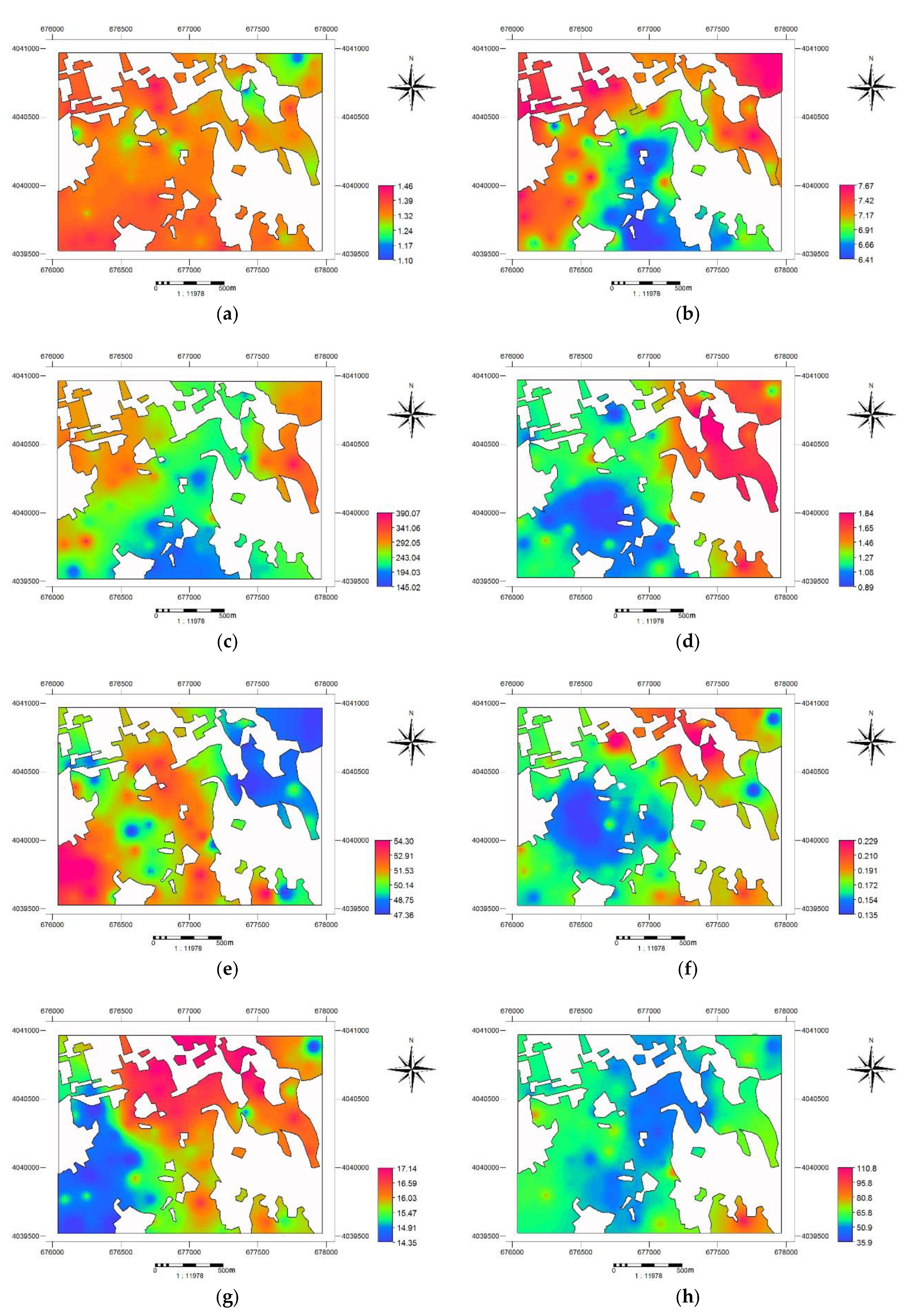
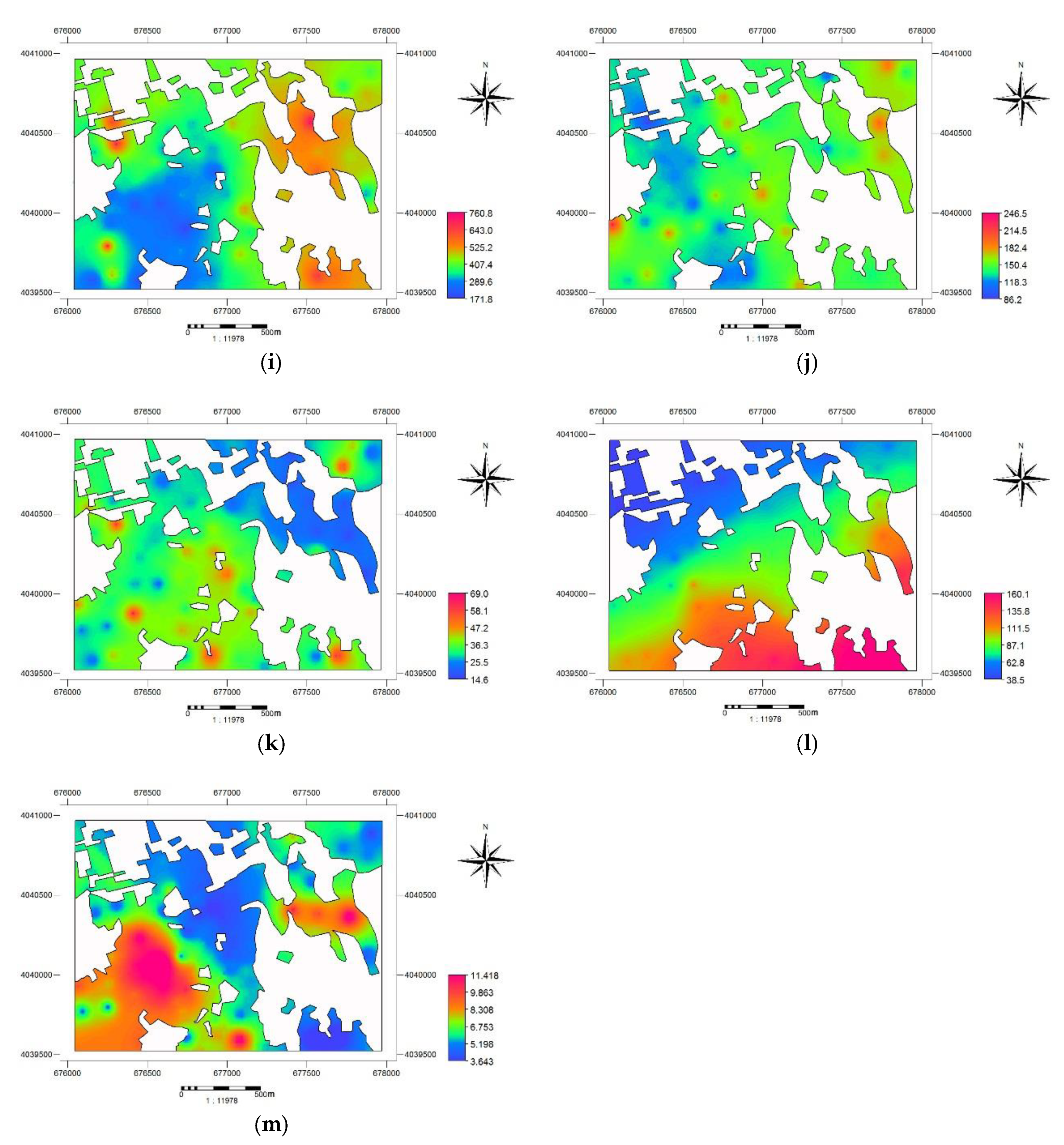
3.2. Spatial Variability Analysis

The accuracy of the interpolation method (e.g., IDW) for soil and terrain properties is presented in

Table 3. Accuracy of the inverse distance weighting (IDW) method for interpolation of soil and terrain properties.

Variable	Weighting Power	R2	nRMSE	CRM
BD	3	0.74	5.2	0.04
pH	2	0.73	5.4	0.04
EC	5	0.83	3.4	0.03
SOC	2	0.79	8.4	0.07
Cl	3	0.81	3.8	0.03
TN	3	0.79	4.2	0.03
CEC	4	0.77	13.8	0.11
Mres4	5	0.84	3.2	0.03
Cmic	4	0.84	6.4	0.05
Kav	4	0.79	4.2	0.03
Pav	2	0.86	5.6	0.05
Elevation (m)	5	0.92	3.2	0.03
Slope (%)	3	0.85	9.0	0.08

BD, soil bulk density (g cm⁻³); EC, electrical conductivity (µS cm⁻¹); SOC, total soil organic carbon (%); Cl, clay (in the 0–30 cm soil surface layer (%)); TN, total nitrogen (%); K_av, available potassium (mg kg⁻¹); Mres4, soil respiration at the 4th day incubated at 30 °C (mg CO₂–C kg⁻¹ soil d⁻¹); Cmic, microbial biomass carbon (mg C kg⁻¹ soil); CEC, cation exchange capacity (meq 100 g⁻¹ soil); P_av, available phosphorus (mg kg⁻¹); R², coefficient of determination; nRMSE, normalized root mean square error; and CRM, coefficient of residual mass.

. Based on validation criteria, the highest and lowest accuracy were obtained for the elevation (R² = 0.92) and pH (R² = 0.73), respectively. The interpolation results for all terrain properties except for CEC (nRMSE = 13.8) interpolated as excellent prediction [45]. Furthermore, all properties interpolated with overestimation (positive CRM) in comparison to the observed data, as shown in Table 3.

Figure 2 shows the spatial distribution maps of all soil properties and topographic variables. BD shows no apparent spatial pattern with only small pitches in the northwest of the study area, as shown in Figure 2a. The spatial distributions of soil pH and EC, as shown in Figure 2b,c, and elevation, as shown in Figure 2l, were almost similar, with greater values of pH in the north where lower elevation occurred in the study area (r = −0.693, p < 0.01). The lateral downward movement of decalcified solution within the soils may lead to the enrichment of calcium carbonated in low-laying areas. Soil organic carbon, as shown in Figure 2d, and clay, as shown in Figure 2c, showed opposite spatial patterns (r = −0.654, p < 0.01), whereas SOC showed a similar pattern with TN, as shown in Figure 2f, and CEC, as shown in Figure 2g (r = 0.610, p < 0.01 and r = 0.590, p < 0.01, respectively). The upland soils, which are located in the margin of the study area and adjacent to existing forests, have higher SOC and CEC values, indicating the recent conversion of land use change from forests to citrus plantations. The K_av values displayed a homogeneous spatial distribution pattern, as shown in Figure 2j. It could be attributed to the illite clay minerals that are the most clay-dominant minerals in the study area [53]. The P_av showed low content in the west to northwest and almost homogeneous spatial patterns for the rest of the study area, as shown in Figure 2k.

3.3. Principal Component Analysis (PCA)

The PCA was used to reduce the dimensionality and summarize the variability of soil and terrain variables. Due to the high correlation between soil properties and topographic attributes, as shown in Table 2, PCA is an appropriate method to aggregate the effect of the parameters [14,44,54]. The PCs with eigenvalues greater than 1.0 could explain 78.66% of the dataset variability in the study area, as shown in

Table 4. Results of the principal component analysis (PCA) applied to the soil physicochemical properties and topographic attributes in the studied area.

PCs a	PC1	PC2	PC3	PC4
Eigenvalue	4.26	2.45	1.61	1.11
Percent	35.52	20.44	13.46	9.25
Cumulative percent	35.52	55.96	69.41	78.66
Eigenvectors
BD	0.37	−0.83	0.19	0.16
pH	0.44	−0.71	0.42	0.22
EC	0.88	0.17	0.22	−0.20
SOC	−0.63	0.06	−0.13	0.52
Cl	0.72	0.31	−0.28	0.00
TN	0.50	0.30	0.22	0.11
Kav	0.21	0.36	0.73	0.39
Mres4	0.85	0.20	0.16	0.06
Cmic	0.68	0.15	−0.57	0.07
CEC	−0.69	0.26	0.09	0.35
Pav	−0.18	0.84	0.38	−0.18
Elevation	−0.48	−0.25	0.41	−0.63
Slope	0.37	−0.83	0.19	0.16

^a Principal component. Underlined factor loadings are considered highly weighted. BD, soil bulk density (g cm⁻³); EC, electrical conductivity (µS cm⁻¹); SOC, total soil organic carbon (%); Cl, clay (%); TN, total nitrogen (%); K_av, available potassium (mg kg⁻¹); Mres4, soil respiration at the 4th day incubated at 30 °C (mg CO₂–C kg⁻¹ soil d⁻¹); Cmic, microbial biomass carbon (mg C kg⁻¹ soil); CEC, cation exchange capacity (meq 100 g⁻¹ soil); P_av, available phosphorus (mg kg⁻¹).

. The PC1 explained the majority of the total data variance (35.52%) with a positive loading factor for EC, clay, TN, Mres4, and Cmic, and a negative loading factor for SOC and CEC. The PC2 explained 20.44% of the total variance and included BD, pH, and slope (negative loading factors), and P_av (positive loading factor). The PC3 included K_av, with a positive loading factor, which explained an additional 13.46% of the total variance in the dataset. The last PC (PC4) explained 9.25% of the data variability with a negative loading factor for elevation, as shown in Table 4. Therefore, the first four components (PC1, PC2, PC3, and PC4) were used to delineate the MZs for the commercial citrus plantation here. Behera et al. [42] delineated soil MZs of oil palm plantations by using PCA and fuzzy c-means in India and found that three PCs could explain 60.31% of soil property variation. Moreover, several studies have shown that PCA is an effective method to discriminate and delineate soils [44,55]. Therefore, the PCA analysis combined twelve input variables into four PCs, accounting for the majority of spatial variability in these properties.

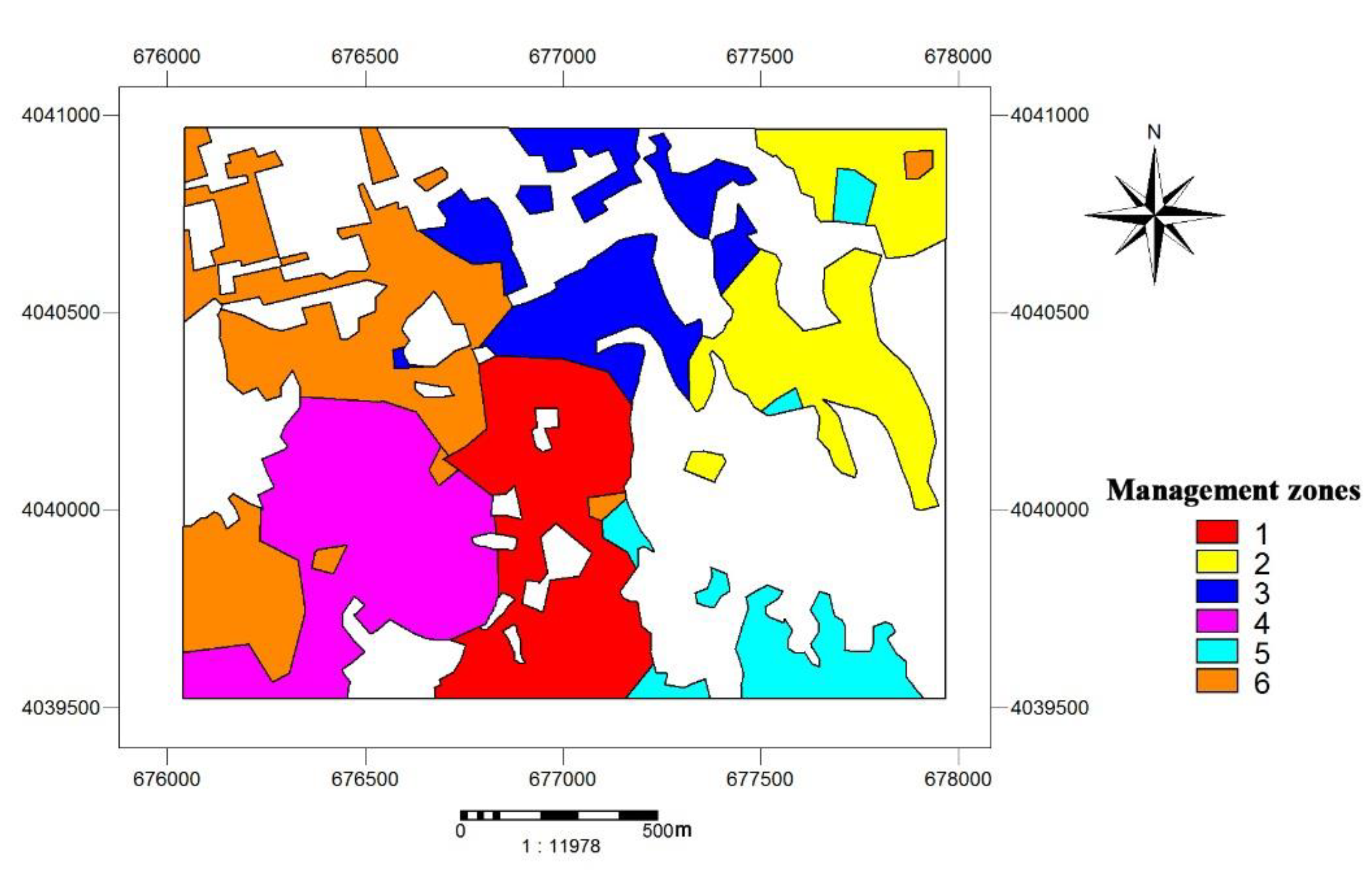
3.4. Clustering Analysis

A cluster analysis was applied to classify the four PCs into MZs. The MZA software was used to perform the fuzzy c-means cluster algorithm on the scores of the four PCs to define the optimum number of MZs. This method allows us to differentiate different zones with a similar value of properties and higher differences between them. To obtain the optimum number of MZs, the NCE and FPI parameters were calculated and plotted, as shown in Figure 3, against the number of clusters (or MZs) [46]. Therefore, when the FPI and NCE values were minimal, the optimal number of MZs can be identified, as shown in Figure 3. In this study, six different management zones were finally identified as the optimum number of MZs, as shown in Figure 3.

Figure 4 shows the spatial distribution map of the six delineated MZs in the study area. In each delineated MZ, the measured soil properties and topographic attributes present the lowest variance and highest degree of membership [9]. Thus, in each zone, different management practices, such as nutrient application, can be carried out to increase crop production while decreasing the costs.

Several studies stated that the analysis of variance is an effective method to assess the differences between the delineated zones [9,14,15,17,42]. Therefore, the one-way ANOVA was carried out to evaluate the effectiveness of PCA and fuzzy c-means cluster algorithm combination to delineate MZs and also its spatial variability.

There were significant differences (p < 0.05) between all soil and terrain attributes except for BD among the six MZs, as shown in Table 4. Since the agricultural practices and machinery movement are similar in all MZ zones, the soil pore distribution (e.g., macropore and mesopore volumes) remains constant and did not show significant differences. Hosseini et al. [49,56] proved that agricultural practices and soil compaction were the main reasons for the BD variation and differences in the farms. The slope percentage only showed a significant difference in MZ4 in comparison to other MZs. The MZ4 with the lowest clay, TN, K_av, Cmic, CEC, and lower SOC and P_av values could have lower potential soil fertility than others, as shown in Table 4, suggesting more chemical fertilizers are needed in this zone (particularly nitrogen). Thus, this MZ has a great potential for environmental risk via nitrogen leaching through the soil profiles and also nitrogen load in soil surface run-off with highest slope among the other zones. The MZ1, MZ2, MZ4, and MZ6 had a mean value of TN less than the limiting critical value for the citrus tree. Moreover, all of the delineated MZs had K_av deficiency, while only MZ2 had P_av deficiency, as shown in Table 1 and Table 4 [27]. In general, the ranking was MZ5 > MZ2 > MZ6 > MZ1 > MZ3 > MZ4 in terms of soil fertility according to all the soil properties examined, as shown in

Table 5. Mean values of each management zone and variance analysis for all studied soil physicochemical properties and topographic attributes.

Zone	n	BD	pH	EC	SOC	Clay	TN	Kav	Mres4	Cmic	CEC	Pav	Elevation (m)	Slope (%)
MZ1	9	1.32a	6.2d	154e	1.06b	53.0a	0.162bc	136ab	44.6d	310.3c	16.1bc	45.4a	109a	3.8b
MZ2	9	1.29a	7.5ab	334a	1.77a	47.9b	0.183abc	155a	68.49ab	545.9ab	16.2ab	19.5b	91a	7.0b
MZ3	6	1.33a	7.4abc	232cd	1.46ab	49.4ab	0.233a	149ab	43.59d	384.8bc	17.6a	22.9b	60b	3.7b
MZ4	12	1.37a	6.8c	197de	1.08b	49.1b	0.148c	110b	51.99cd	228.2c	14.2d	27.0b	102a	13.0a
MZ5	10	1.34a	7.0bc	271bc	1.36ab	51.3ab	0.202ab	178a	81.11a	581.4a	15.0cd	48.2a	105a	4.1b
MZ6	11	1.33a	7.6a	314ab	1.16b	52.7a	0.149c	148ab	63.32bc	361.9c	15.9bc	32.9bc	64b	4.8b
Significance	(Pr value)	0.7806	0.0108	0.0001	0.01	0.0042	0.01	0.0000	0.0003	0.0036	0.0037	0.0000	0.0067	0.0000

BD, soil bulk density (g cm⁻³); EC, electrical conductivity (µS cm⁻¹); SOC, total soil organic carbon (%); Cl, clay (in the 0–25 cm soil surface layer (%)); TN, total nitrogen (%); K_av, available potassium (mg kg⁻¹); Mres4, soil respiration at the 4th day incubated at 30 °C (mg CO₂–C kg⁻¹ soil d⁻¹); Cmic, microbial biomass carbon (mg C kg⁻¹ soil); CEC, cation exchange capacity (meq 100 g⁻¹ soil); P_av, available phosphorus (mg kg⁻¹). Means with the same letter are not significantly different at the 0.05 probability level based on the least significant difference test.

. This finding is important for deciding the amount of fertilizers to be added to the soils in different zones. It emphasizes the needed site-specific management of citrus garden soils for sustainable citrus productivity and, in turn, for lowering the environmental hazards by ununiformed application of chemical fertilizers [26,57].

3.5. Economic Analysis of Delineated Zones

The economic analysis of fertilizer savings was performed in the MZs in comparison with uniform fertilization management. Based on the results, MZ5 and MZ4 had the lowest and highest total cost of chemical fertilizers per tree and animal manure, respectively, and the ranking was MZ5 < MZ2 < MZ6 < MZ1 < MZ3 < MZ4, as shown in

Table 6. Economic analysis of the fertilizer savings in the management zones by comparing the difference between site-specific fertilization and uniform management.

	Fertilizer #					Total Cost per Tree (Iranian Rials)	RC (%) †
	Nitrogen	Phosphorus	Potassium	Sulfur	Rotted Animal Manure
Price Per kg (Iranian Rials)	14,000	20,000	24,000	12,000	5000	–	–
Zone	Kg Fertilizer per Tree
MZ1	0.500	0.050	0.875	0.000	17.50	116,500	29.4
MZ2	0.250	0.225	0.750	1.875	10.00	98,500	9.44
MZ3	0.375	0.125	0.775	1.875	13.75	117,600	30.6
MZ4	0.500	0.125	1.000	0.000	17.50	121,000	34.4
MZ5	0.375	0.050	0.625	0.000	13.75	90,000	0.00
MZ6	0.300	0.050	0.775	0.000	15.00	98,800	9.77

^† To show the variation among the zones, we used Zone 5 as a reference zone and the other zones were compared with Zone 5 based on the relative cost of changes [RC, % = ((X × 100)/Y) –100 suggested by Bakhshandeh et al. [38]. ^# Source of chemical fertilizers: nitrogen (urea, 46%), phosphorus (triple superphosphate, 46%), potassium (potassium sulfate, 46%), and sulfur (with 50% purity).

. On the other hand, if MZ5 is defined as a reference zone due to the lowest cost needed, other zones, therefore, can be compared to this zone using the RC values. In fact, MZ4, MZ3, MZ1, MZ6, and MZ2 required 34.4, 30.6, 29.4, 9.77, and 9.44% more costs than MZ5 for achieving similar productivity, respectively, as shown in Table 6. The MZ delineation allows for the utilization of different doses of fertilizers, and cultural and irrigation practices as well that could lead to a decline in operational costs. Thus, this result highlighted that the combination of PCA and fuzzy c-means analysis could be used to effectively delineate MZs for soil nutrient management to maximize crop production and minimize its costs [42]. Our finding is also supported by other studies that the application of fertilizers can be based on MZ delineation [15,17,24,58].

Although the MZ delineation based on soil and terrain attributes (topographic attributes) had good accuracy and was economically and environmentally sound, it is time-consuming and to some extent costly because of soil analysis [10]. Therefore, when soil data with reasonable distribution is not available, and also a time-efficient and cost-effective approach are needed, using a combination of remote sensing data and topographic attributes (environmental covariates with high resolution) can potentially be an alternative approach to delineate MZs in agricultural farms [59], but it needs to be verified in this region to decrease the methodology costs as much as possible.

4. Conclusions

The current study shows that the spatial variations of some selected soil properties and terrain attributes could be a possible approach to delineate soil MZs in commercial citrus plantations. The high correlation of soil properties and terrain attributes indicated considerable spatial variability and that site-specific nutrient management is needed in this region. The optimal number of MZs by PCA and fuzzy c-means clustering was six and a one-way ANOVA showed a significant heterogeneity variation among different MZs. In terms of cost-efficiency analysis, MZ5 and MZ4 showed the lowest and highest total operational cost. Therefore, the simplicity and cost-effectiveness of numerical methods, such as geostatistical tools, PCA, and fuzzy c-means clustering, could be an initial step to utilize fertilizers and reduce the cultural cost in precision agriculture management. However, this has to be performed using an inexpensive technique and input data because the profitability in these types of farms are very low, so owners need a cheap, effective, and reliable method to know which zones have similar production potential. Consequently, remote sensing and topographic variables could be suggested for future studies to reduce the cost of soil MZs more and more at the farm scale when high-resolution (e.g., 1 or 5 m) terrain attributes are available.

References

1. Ladanyia, M.; Ladaniya, M. Citrus Fruit: Biology, Technology and Evaluation; Academic Press: Cambridge, MA, USA, 2010. [Google Scholar]
2. Goldschmidt, E.E.; Koch, K.E. Citrus. In Photoassimilate Distribution Plants and Crops Source-Sink Relationships; Routledge: Abingdon, UK, 2017; pp. 797–824. [Google Scholar]
3. Liu, Y.; Heying, E.; Tanumihardjo, S.A. History, global distribution, and nutritional importance of citrus fruits. Compr. Rev. Food Sci. Food Saf. 2012, 11, 530–545. [Google Scholar] [CrossRef]
4. FAO. Citrus Fruit-Fresh and Processed Statistical Bulletin 2016; Food and Agriculture Organization of the United Nations: Rome, Italy, 2017; p. 66. [Google Scholar]
5. Tripathi, R.; Nayak, A.; Shahid, M.; Lal, B.; Gautam, P.; Raja, R.; Mohanty, S.; Kumar, A.; Panda, B.; Sahoo, R. Delineation of soil management zones for a rice cultivated area in eastern India using fuzzy clustering. Catena 2015, 133, 128–136. [Google Scholar] [CrossRef]
6. Wan, S.; Zhang, C.; Chen, Y.; Zhao, J.; Zhu, X.; Wu, J.; Zhou, L.; Lin, Y.; Liu, Z.; Fu, S. Interactive effects of understory removal and fertilization on soil respiration in subtropical Eucalyptus plantations. J. Plant Ecol. 2015, 8, 284–290. [Google Scholar] [CrossRef] [Green Version]
7. Dobermann, A.; Oberthür, T. Fuzzy mapping of soil fertility—A case study on irrigated riceland in the Philippines. Geoderma 1997, 77, 317–339. [Google Scholar] [CrossRef]
8. Castrignanò, A.; Buttafuoco, G.; Quarto, R.; Parisi, D.; Rossel, R.V.; Terribile, F.; Langella, G.; Venezia, A. A geostatistical sensor data fusion approach for delineating homogeneous management zones in Precision Agriculture. Catena 2018, 167, 293–304. [Google Scholar] [CrossRef]
9. Oldoni, H.; Terra, V.S.S.; Timm, L.C.; Júnior, C.R.; Monteiro, A.B. Delineation of management zones in a peach orchard using multivariate and geostatistical analyses. Soil Tillage Res. 2019, 191, 1–10. [Google Scholar] [CrossRef]
10. Chang, D.; Zhang, J.; Zhu, L.; Ge, S.-H.; Li, P.-Y.; Liu, G.-S. Delineation of management zones using an active canopy sensor for a tobacco field. Comput. Electron. Agric. 2014, 109, 172–178. [Google Scholar] [CrossRef]
11. Gili, A.; Álvarez, C.; Bagnato, R.; Noellemeyer, E. Comparison of three methods for delineating management zones for site-specific crop management. Comput. Electron. Agric. 2017, 139, 213–223. [Google Scholar] [CrossRef]
12. Metwally, M.S.; Shaddad, S.M.; Liu, M.; Yao, R.-J.; Abdo, A.I.; Li, P.; Jiao, J.; Chen, X. Soil Properties Spatial Variability and Delineation of Site-Specific Management Zones Based on Soil Fertility Using Fuzzy Clustering in a Hilly Field in Jianyang, Sichuan, China. Sustainability 2019, 11, 7084. [Google Scholar] [CrossRef] [Green Version]
13. Ortega, R.A.; Santibáñez, O.A. Determination of management zones in corn (Zea mays L.) based on soil fertility. Comput. Electron. Agric. 2007, 58, 49–59. [Google Scholar] [CrossRef]
14. Xin-Zhong, W.; Guo-Shun, L.; Hong-Chao, H.; Zhen-Hai, W.; Qing-Hua, L.; Xu-Feng, L.; Wei-Hong, H.; Yan-Tao, L. Determination of management zones for a tobacco field based on soil fertility. Comput. Electron. Agric. 2009, 65, 168–175. [Google Scholar] [CrossRef]
15. Davatgar, N.; Neishabouri, M.; Sepaskhah, A. Delineation of site specific nutrient management zones for a paddy cultivated area based on soil fertility using fuzzy clustering. Geoderma 2012, 173, 111–118. [Google Scholar] [CrossRef]
16. Jiang, H.-L.; Liu, G.-S.; Liu, S.-D.; Li, E.-H.; Wang, R.; Yang, Y.-F.; Hu, H.-C. Delineation of site-specific management zones based on soil properties for a hillside field in central China. Arch. Agron. Soil Sci. 2012, 58, 1075–1090. [Google Scholar] [CrossRef]
17. Schenatto, K.; de Souza, E.G.; Bazzi, C.L.; Gavioli, A.; Betzek, N.M.; Beneduzzi, H.M. Normalization of data for delineating management zones. Comput. Electron. Agric. 2017, 143, 238–248. [Google Scholar] [CrossRef]
18. Keshavarzi, A.; Kumar, V.; Bottega, E.L.; Rodrigo-Comino, J. Determining land management zones using pedo-geomorphological factors in potential degraded regions to achieve land degradation neutrality. Land 2019, 8, 92. [Google Scholar] [CrossRef] [Green Version]
19. Fu, Q.; Wang, Z.; Jiang, Q. Delineating soil nutrient management zones based on fuzzy clustering optimized by PSO. Math. Comput. Model. 2010, 51, 1299–1305. [Google Scholar] [CrossRef]
20. Jiang, H.-L.; Liu, G.-S.; Wang, R.; Liu, S.-D.; Han, F.-G.; Yang, Y.-F.; Ye, X.-F.; Zhang, Q.-J.; Wang, X.-J.; Wang, Z.-H. Delineating site-specific quality-based management zones for a tobacco field. Soil Sci. 2011, 176, 206–212. [Google Scholar] [CrossRef]
21. Zhao, C.; Fu, S.; Mathew, R.P.; Lawrence, K.S.; Feng, Y. Soil microbial community structure and activity in a 100-year-old fertilization and crop rotation experiment. J. Plant Ecol. 2015, 8, 623–632. [Google Scholar] [CrossRef] [Green Version]
22. McKinion, J.; Jenkins, J.; Akins, D.; Turner, S.; Willers, J.L.; Jallas, E.; Whisler, F. Analysis of a precision agriculture approach to cotton production. Comput. Electron. Agric. 2001, 32, 213–228. [Google Scholar] [CrossRef]
23. Hedley, C. The role of precision agriculture for improved nutrient management on farms. J. Sci. Food Agric. 2015, 95, 12–19. [Google Scholar] [CrossRef]
24. Aggelopooulou, K.; Castrignanò, A.; Gemtos, T.; De Benedetto, D. Delineation of management zones in an apple orchard in Greece using a multivariate approach. Comput. Electron. Agric. 2013, 90, 119–130. [Google Scholar] [CrossRef]
25. Valente, D.S.M.; Queiroz, D.M.D.; Pinto, F.D.A.D.C.; Santos, N.T.; Santos, F.L. Definition of management zones in coffee production fields based on apparent soil electrical conductivity. Sci. Agric. 2012, 69, 173–179. [Google Scholar] [CrossRef] [Green Version]
26. Peralta, N.R.; Costa, J.L.; Balzarini, M.; Franco, M.C.; Córdoba, M.; Bullock, D. Delineation of management zones to improve nitrogen management of wheat. Comput. Electron. Agric. 2015, 110, 103–113. [Google Scholar] [CrossRef]
27. Kangarshahi, A.A.; Akhlaghi Amiri, N. Advanced and Applied Citrus Nutrition; Agricultural Education and Promotion Publications: Tehran, Iran, 2015; Volume I, p. 312. [Google Scholar]
28. Soil Survey Staff. Keys to Soil Taxonomy, 12th ed.; USDA-Natural Resources Conservation Service: Washington, DC, USA, 2014.
29. Mallarino, A. Management Zones Soil Sampling: A Better Alternative to Grid and Soil Type Sampling? Iowa State University Digital Press: Ames, IA, USA, 2001. [Google Scholar]
30. Nelson, D.W.; Sommers, L.E. Total carbon, organic carbon, and organic matter. Methods Soil Anal. Part 3 Chem. Methods 1996, 5, 961–1010. [Google Scholar]
31. Blake, G.R.; Hartge, K.H. Bulk density. In Methods of Soil Analysis. Part 1. Physical and Mineralogical Methods, 2nd ed.; Klute, A., Ed.; ASA; SSSA: Madison, WI, USA, 1986; pp. 363–382. [Google Scholar]
32. McLean, E.; Mulvaney, C. Soil pH and lime requirement. In Methods of Soil Analysis. Part 2. Chemical and Microbiological Properties; Wiley Online Library: Hoboken, NJ, USA, 1982. [Google Scholar]
33. Rhoades, J. Soluble salts. In Methods of Soil Analysis Part 2: Chemical and Microbiological Properties; Page, A.L., Miller, R.H., Keeney, D.R., Eds.; American Society of Agronomy: Madison, WI, USA, 1982; pp. 167–178. [Google Scholar]
34. Bremner, J. Nitrogen–total. In Methods of Soil Analyses, Part 3, Chemical Methods; Sparks, D.L., Ed.; Soil Science Society of America and American Society of Agronomy: Madison, WI, USA, 1996; pp. 1085–1122. [Google Scholar]
35. Estefan, G.; Sommer, R.; Ryan, J. Methods of soil, plant, and water analysis. In A Manual for the West Asia and North Africa Region; ICARDA: Beirut, Lebanon, 2013; Volume 3. [Google Scholar]
36. Olsen, S.R. Estimation of Available Phosphorus in Soils by Extraction with Sodium Bicarbonate; US Department of Agriculture: Washington, DC, USA, 1954.
37. Mc Lean, E.; Watson, M. Soil measurements of plant-available potassium. In Potassium in Agriculture; Wiley Online Library: Hoboken, NJ, USA, 1985; pp. 277–308. [Google Scholar]
38. Bakhshandeh, E.; Francaviglia, R.; Renzi, G. A cost and time-effective method to evaluate soil microbial respiration for soil quality assessment. Appl. Soil Ecol. 2019, 140, 121–125. [Google Scholar] [CrossRef]
39. Vance, E.D.; Brookes, P.C.; Jenkinson, D.S. An extraction method for measuring soil microbial biomass C. Soil Biol. Biochem. 1987, 19, 703–707. [Google Scholar] [CrossRef]
40. Institute, S. Base SAS 9.4 Procedures Guide; SAS Institute: Cary, NC, USA, 2015. [Google Scholar]
41. Warrick, A.W.; Nielsen, D.R. Spatial variability of soil physical properties the soil. In Applications of Soil Physics; Hill, D., Ed.; Academic Press: New York, NY, USA, 1980; pp. 319–344. [Google Scholar]
42. Behera, S.K.; Mathur, R.K.; Shukla, A.K.; Suresh, K.; Prakash, C. Spatial variability of soil properties and delineation of soil management zones of oil palm plantations grown in a hot and humid tropical region of southern India. Catena 2018, 165, 251–259. [Google Scholar] [CrossRef]
43. Rodrigo-Comino, J.; Keshavarzi, A.; Zeraatpisheh, M.; Gyasi-Agyei, Y.; Cerdà, A. Determining the best ISUM (Improved stock unearthing Method) sampling point number to model long-term soil transport and micro-topographical changes in vineyards. Comput. Electron. Agric. 2019, 159, 147–156. [Google Scholar] [CrossRef]
44. Zeraatpisheh, M.; Ayoubi, S.; Sulieman, M.; Rodrigo-Comino, J. Determining the spatial distribution of soil properties using the environmental covariates and multivariate statistical analysis: A case study in semi-arid regions of Iran. J. Arid Land 2019, 11, 551–566. [Google Scholar] [CrossRef] [Green Version]
45. Jamieson, P.; Porter, J.; Wilson, D. A test of the computer simulation model ARCWHEAT1 on wheat crops grown in New Zealand. Field Crops Res. 1991, 27, 337–350. [Google Scholar] [CrossRef]
46. Fridgen, J.J.; Kitchen, N.R.; Sudduth, K.A.; Drummond, S.T.; Wiebold, W.J.; Fraisse, C.W. Management zone analyst (MZA). Agron. J. 2004, 96, 100–108. [Google Scholar] [CrossRef]
47. Odeh, I.; McBratney, A.; Chittleborough, D. Soil pattern recognition with fuzzy-c-means: Application to classification and soil-landform interrelationships. Soil Sci. Soc. Am. J. 1992, 56, 505–516. [Google Scholar] [CrossRef]
48. Soil and Water Research Institute of Iran. 2019. Available online: http://www.swri.ir/ (accessed on 1 October 2019).
49. Hosseini, M.; Movahedi Naeini, S.A.R.; Dehghani, A.A.; Zeraatpisheh, M. Modeling of soil mechanical resistance using intelligent methods. J. Soil Sci. Plant Nutr. 2018, 18, 939–951. [Google Scholar] [CrossRef] [Green Version]
50. Sumner, M.E. Handbook of Soil Science; CRC Press: Boca Raton, FL, USA, 1999. [Google Scholar]
51. Wilding, L.P.; Dress, L.R. Application of geostatistics to spatial studies of soil. In Advances in Agronomy; Trangmar, B.B., Yost, R.S., Uehara, G., Eds.; Academic Press, Inc.: Orlando, FL, USA, 1983; Volume 38. [Google Scholar]
52. Karaman, M.; Ersahin, S.; Durak, A. Spatial variability of available phosphorus and site specific phosphorus fertilizer recommendations in a wheat field. In Plant Nutrition–Food Security and Sustainability of Agro-Ecosystems Through Basic and Applied Research; Horst, W.J., Ed.; Kluwer Academic Publishers: Dordrecht, The Netherlands, 2001. [Google Scholar]
53. Bahmanyar, M.; Abtahi, A.; Banaee, M. Soil landscape relationshipps between different physiographic units in tejan catchment (northern iran). Iran Agric. Res. 1999, 18, 107–124. [Google Scholar]
54. Yao, R.-J.; Yang, J.-S.; Zhang, T.-J.; Gao, P.; Wang, X.-P.; Hong, L.-Z.; Wang, M.-W. Determination of site-specific management zones using soil physico-chemical properties and crop yields in coastal reclaimed farmland. Geoderma 2014, 232, 381–393. [Google Scholar] [CrossRef]
55. Metternicht, G.; Zinck, J. Remote sensing of soil salinity: Potentials and constraints. Remote Sens. Environ. 2003, 85, 1–20. [Google Scholar] [CrossRef]
56. Hosseini, M.; Naeini, S.A.M.; Dehghani, A.A.; Khaledian, Y. Estimation of soil mechanical resistance parameter by using particle swarm optimization, genetic algorithm and multiple regression methods. Soil Tillage Res. 2016, 157, 32–42. [Google Scholar] [CrossRef]
57. Bullock, D.S.; Ruffo, M.L.; Bullock, D.G.; Bollero, G.A. The value of variable rate technology: An information-theoretic approach. Am. J. Agric. Econ. 2009, 91, 209–223. [Google Scholar] [CrossRef]
58. Gavioli, A.; de Souza, E.G.; Bazzi, C.L.; Schenatto, K.; Betzek, N.M. Identification of management zones in precision agriculture: An evaluation of alternative cluster analysis methods. Biosyst. Eng. 2019, 181, 86–102. [Google Scholar] [CrossRef]
59. Breunig, F.M.; Galvão, L.S.; Dalagnol, R.; Dauve, C.E.; Parraga, A.; Santi, A.L.; Della Flora, D.P.; Chen, S. Delineation of management zones in agricultural fields using cover–crop biomass estimates from PlanetScope data. Int. J. Appl. Earth Obs. Geoinf. 2020, 85, 102004. [Google Scholar] [CrossRef]
Figure 1. Location of the study area in Iran (a); Mazandaran Province (b); map and the sampling experimental grid established in the orchard (Citrus spp.) constituted of 57 sampling points (c); and a photograph of the citrus plantation (d).
Sustainability 12 05809 g001
Figure 2. Spatial distribution maps for all studied attributes in the 0–30 cm soil layer: (a) soil bulk density (g cm−3); (b) pH; (c) electrical conductivity (µS cm−1); (d) soil organic carbon (%); (e) clay (%); (f) total nitrogen (%); (g) cation exchange capacity (meq 100 g−1 soil); (h) soil respiration at the 4th day incubated at 30 °C (mg CO2–C kg−1 soil d−1); (i) microbial biomass carbon (mg C kg−1 soil), (j) available potassium (mg kg−1); (k) available phosphorus (mg kg−1); (l) elevation (m); and (m) slope (%).
Sustainability 12 05809 g002aSustainability 12 05809 g002b
Figure 3. Calculated fuzziness performance index (FPI) and normalized classification entropy (NCE) for the different number of cluster classes.
Sustainability 12 05809 g003
Figure 4. Spatial distribution map for the resulting management zones.
Sustainability 12 05809 g004