Abstract
Agricultural production in the Texas High Plains (THP) relies heavily on irrigation and is susceptible to drought due to the declining availability of groundwater and climate change. Therefore, it is meaningful to perform an overview of possible climate change scenarios to provide appropriate strategies for climate change adaptation in the THP. In this study, spatio-temporal variations of climate data were mapped in the THP during 2000–2009, 2050–2059, and 2090–2099 periods using 14 research-grade meteorological stations and 19 bias-corrected General Circulation Models (GCMs) under representative concentration pathway (RCP) scenarios RCP 4.5 and 8.5. Results indicated different bias correction methods were needed for different climatic parameters and study purposes. For example, using high-quality data from the meteorological stations, the linear scaling method was selected to alter the projected precipitation while air temperatures were bias corrected using the quantile mapping method. At the end of the 21st century (2090–2099) under the severe CO2 emission scenario (RCP 8.5), the maximum and minimum air temperatures could increase from 3.9 to 10.0 °C and 2.8 to 8.4 °C across the entire THP, respectively, while precipitation could decrease by ~7.5% relative to the historical (2000–2009) observed data. However, large uncertainties were found according to 19 GCM projections.
1. Introduction
Future climatic changes may have significant impacts on water resources and food production at regional and global scales [1,2]. The increase in human population places growing demands on existing resources and has led to destruction of forests, increased combustion of fossil fuels, and increased agricultural management intensity and livestock production, which has raised atmospheric CO2 concentration [3,4]. The increased air CO2 concentration can trap heat and warm the earth’s surface, which can further alter the amount, intensity, pattern, and duration of rainfall [5]. The increase in air temperatures and change in precipitation distribution may have significant negative impacts on water resources and agricultural production in semi-arid or arid regions [6,7,8,9,10].
The semi-arid Texas High Plains (THP) in the United States (U.S.) was formed as a result of alluvial sediment depositions brought by rivers that originated from the Rocky Mountains [11,12]. The THP is a relatively treeless, agricultural and rangeland dominant, and windy region [13]. It is one of the most intensive agricultural regions in the world, and cotton (Gossypium hirsutum L.) is a major crop grown in the THP region. The cotton planting area is approximately 32% of the U.S. total in 2019 [14]. Corn (Zea mays L.) is the major irrigated crop, and several counties in the THP have reported the largest average corn yields in the nation [14]. The potential climate change phenomena of increased temperatures and decreased precipitation can be the most important threat in the agricultural sector affecting the semi-arid THP. For instance, the increase of future temperatures can cause a reduced maturity period of corn, which could decrease time duration of corn to use solar radiation and assimilate CO2 and adversely influence the accumulation of corn biomass and final yield [14,15,16,17]. Climate change adaptation, such as alternative planting dates, land use change, and stress tolerant cultivars, can be time-consuming and costly. However, advance study and planning will be beneficial in mitigation of the adverse impacts of climate change. Therefore, assessing climate change trends under current and future climate scenarios enables not only the development of best agricultural management practices (BMPs) with potential adoption rates and strategies in the future, but also the awareness, preparation, and precautionary actions of possible associated environmental issues.
There is a growing number of studies quantifying climate change using General Circulation Models (GCMs) [18,19,20,21,22]. In addition, GCM ensemble forecasting is a technique for the representation of uncertainties in predicting future climate scenarios. A GCM ensemble should frame the uncertainty and help to derive decisions from the forecast. Working with multi-GCM ensembles is well-established in climate forecasting [23]. However, the innovation of this study is not only in using 19 GCMs and their ensembles, but also using long-term measured daily climate data obtained from a well-maintained, research-grade, and agricultural production-based network of appropriately sited meteorological stations to bias correct the GCM projections. Therefore, the findings of this study represent the future climatic change under an agricultural production system scenario instead of an urban, forest, or other ecological systems.
The overall goal of this study was to analyze the spatio-temporal distribution of climate data in the agricultural production system in the THP. Specifically, this study aimed to (1) map the spatial and temporal patterns of precipitation, maximum air temperature, and minimum air temperature during 2000–2009, 2050–2059, and 2090–2099 time intervals using geospatial analysis; (2) determine the climate change trends and uncertainties for each of the 14 research-grade agro-meteorological stations according to 19 GCM projections; and (3) explore the possible impacts of future climate change on the THP.
2. Materials and Methods
2.1. Study Region and Climate Data
The Texas High Plains includes the Texas Northern High Plains (TNHP) and the Texas Southern High Plains (TSHP), and the total area is approximately 102,300 km2. The TSHP consists of 16 counties extending from northwest of Lubbock to Midland, while the TNHP region is comprised of 25 counties in the northern panhandle of the state. The regional climate in the THP is classified as semi-arid with an average annual rainfall and temperature of ~400 mm and 14 °C, respectively. Agricultural production in this region is water limited and variable, with average evaporation exceeding average precipitation in each month [24]. Cotton is the major cultivated crop in the TSHP. The cotton harvested area in the TSHP is nearly one-quarter of all U.S. cotton [14]. Currently, grain corn is the major irrigated summer crop in the TNHP, and several counties have reported some of the largest average corn yields in the nation [14]. Winter wheat (Triticum aestivum L.) also is an important winter dual-purpose crop grown for both grain production and cattle grazing in the TNHP. The topography of the THP is generally considered flat, and the major soil orders are Alfisols and Mollisols [25].
Long-term (1995–2014) climatic variable data across the THP were collected with the Texas High Plains Evapotranspiration (TXHPET) network (Table 1) [26]. The network of agro-meteorological stations was designed and installed with the purpose of collecting weather measurements for calculating standardized reference evapotranspiration (ETo) values for regional crop irrigation management. Station locations were established in the TXHPET network to represent the major irrigated crop production areas within the region. These values were used in conjunction with planting date-specific crop coefficients for estimating daily crop evapotranspiration (ETc) values for major crops, which were subsequently used for irrigation scheduling by producers within the region [27]. The climate data from the TXHPET network were made available daily to producers via fax initially, and later through a website and e-mail listserv. Station siting was designed to adequately represent regional differences in climate with producers using data from the nearest or most representative station. Each research-grade, agro-meteorological station was maintained in accordance with the American Society of Civil Engineers-Environmental and Water Resources Institute (ASCE-EWRI) specifications [28] and maintained with a quality assurance/quality control (QA/QC) program. All the agro-meteorological stations were situated in sites with well-maintained, cool-season perennial grass. The grass was well irrigated and mowed to a height of three inches to six inches (76 to 152 mm). Data integrity was also confirmed at a regular interval.

Table 1.
Agro-meteorological stations managed by the Texas High Plains Evapotranspiration (TXHPET) network, periods of data records, and elevations in the Texas High Plains.
The major climatic factors collected included precipitation, maximum and minimum air temperatures, solar radiation, wind speed, and relative humidity. In this study, the overlapping climate data from 2000 to 2009 for 14 research-grade, agro-meteorological stations (Bushland, Dalhart, Dimmitt, Earth, Etter, Farwell, Halfway, Lamesa, Lockney from 2006–2010, Lubbock, Morse, Perryton, White Deer, and West Texas A&M University Feedlot from 2001–2009) in the THP were used as the control group (Figure 1 and Table 1). The climatic parameters of interest included in this study for further analysis were daily precipitation, maximum air temperature, and minimum air temperature as they were the parameters available from the future climate projection source (http://gdo-dcp.ucllnl.org/) [29]. The future climate projections of Bias Correction Constructed Analogs version 2 (BCCAv2) with a spatial resolution of 12.5 km2 were downloaded and used in this study. Specifically, from the source (http://gdo-dcp.ucllnl.org/), users can navigate to “Projections: Subset Request” to select the period of the climate data. On the “Step 1.3: Spatial extent selection method” section, users can choose the “Rectangular Area” to manually input the coordinate information. In this way, the users are allowed to download the GCM projections with a spatial resolution of 12.5 km2. To have an appropriate regional cover of the THP with a limited budget, the distance between every two agro-meteorological stations was larger than 12.5 km. Therefore, 14 GCM grids of future climate projections overlapping the 14 research-grade, agro-meteorological stations were downloaded from the future climate projection source for further analysis.
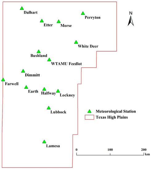
Figure 1.
Meteorological stations in the Texas High Plains.
2.2. Observed Climate Data Pre-processing Using R Programming
Observed climate data review and corrections were processed using the R programming language. First, five variables from compiled daily outputs of each agro-meteorological station, including year, day of year, daily precipitation, daily maximum air temperature, and daily minimum air temperature, were selected out of the total 59 variables. Second, new files were created by selecting data from 1 January 2000 to 31 December 2009. Third, the precipitation data with the English unit (inch) were converted to the SI unit (mm). The R code used for data processing of the research-grade meteorological station data is included in Box A1 (Appendix A). The R code may also be a convenient and useful means for processing similar weather data from other sources such as regional Mesonet data or other ET networks maintained in accordance with the ASCE-EWRI specifications.
2.3. Future Climate Data and Bias Correction Methods
Since future climate trends are heavily dependent on the types of General Circulation Model (GCM) projections [21,30,31], to better represent the variability of the future climate, projected climate data from 19 GCMs were used in this study. They are access1-0, bcc-csm1-1, canesm2, ccsm4, cesm1-bgc, cnrm-cm5, csiro-mk3-6-0, gfdl-esm2g, gfdl-esm2m, inmcm4, ipsl-cm5a-lr, ipsl-cm5a-mr, miroc5, miroc-esm, miroc-esm-chem, mpi-esm-lr, mpi-esm-mr, mri-cgcm3, and noresm1-m [32]. Projected daily precipitation, maximum air temperature, and minimum air temperature from the 19 GCMs during 2000–2099 for the 14 agro-meteorological stations were obtained from the Downscaled Coupled Model Intercomparison Project Phase 5 (CMIP 5) Climate and Hydrology Projections (http://gdo-dcp.ucllnl.org/) [29]. The 19 GCMs projected data under two Representative Concentration Pathway (RCP) emission scenarios, RCP 4.5 (moderate) and RCP 8.5 (severe), were compiled using R (Box A2, Appendix B). Furthermore, the future climate data were bias corrected according to the measured climate data of 2000–2009 using bias correction methods that are external to the future climate projection source. RCP 8.5 is a rising scenario with very high greenhouse gas emissions of 1350 ppm in 2100 [33], while RCP 4.5 is a stabilizing emission scenario with CO2 equivalent concentration of 650 ppm in 2100 [34,35,36] (Table 2).
Table 2.
Description of the representative concentration pathway (RCP) of RCP 4.5 and 8.5.
General Circulation Model data often require bias corrections against the observed data [39,40,41,42]. The bias correction method of quantile mapping is commonly used to adjust the future climate model projections [43,44,45,46]. The aim of quantile mapping is to correct the distribution function of the projected climate data to fit the observed distribution function. A transfer function was created to shift the occurrence distributions of precipitation and air temperatures [45]. The linear scaling method is a simple bias correction method, which operates with monthly correction values based on the differences between observed and simulated values [47]. Bias corrected GCM simulations will entirely agree with the observed data in their average monthly mean values when using the linear scaling method. In this study, the quantile mapping method was implemented for correcting precipitation, maximum air temperature, and minimum air temperature using the bias correction tool—CMhyd (Climate Model data for hydrologic modeling) [48]. In addition, the climate data were bias corrected by linear scaling method using R (Box A3, Appendix C).
2.4. Data Processing, Evaluation, and Analysis
Bias corrected daily precipitation and air temperatures of the 21st century (2000–2099) were reviewed, and two 10-year periods of 2050–2059 and 2090–2099 under both RCP 4.5 and 8.5 scenarios were further used for comparison. The mean values of annual precipitation and daily air temperature were subsequently calculated for analyses. In addition, the bias-corrected precipitation using both linear scaling and quantile mapping methods from 2000 to 2009 for the Halfway station in the THP were extracted to compare with the observed precipitation at the same location and time period to evaluate the performance of the bias correction methods. The detailed design of this climate change study is listed in Table 3. All possible combinations of the data analyses totaled 7980.
Table 3.
Design of the climate change study. GCMs: General Circulation Models. RCPs: Representative Concentration Pathways.
The spatial and temporal trends of climatic variables during the 2000–2009 (measured data), 2050–2059, and 2090–2099 periods in the THP were mapped by producing interpolation maps using GIS software (ArcGIS 10.2, Esri, Redlands, CA, USA). The widely used ordinary kriging method was selected for the interpolation of observed precipitation, maximum and minimum air temperatures, and their relative changes in the middle (2050–2059) and the end (2090–2099) of 21st century. The change uncertainties of future precipitation, maximum air temperature, and minimum air temperature according to 19 GCM projections at each agro-meteorological station were depicted by boxplots using Origin 8.0 software (OriginLab Corporation, Northampton, Massachusetts, USA).
3. Results and Discussion
3.1. Historical Climatic Conditions and Trends in the Texas High Plains
According to the spatial maps, the western part of the THP had lower observed average annual precipitation (2000–2009) than the eastern region (Figure 2). The observed average annual precipitation showed an increasing gradient from the west to east in the THP (Figure 2). The average annual precipitation amounts ranged from 314 to 591 mm across the THP. As for the average annual air temperatures, the northern part of the THP had lower observed maximum temperature than the southern region, while the northwest region exhibited lower minimum air temperature compared to the southeast region (Figure 2). The northernmost agro-meteorological station at Dalhart (36°20′ N) has a clearly different latitude compared to the southernmost Lamesa station (32°47′ N) (Figure 1). The average annual maximum and minimum air temperatures varied from 21.5 to 24.2 °C and 3.4 to 9.3 °C, respectively, across the THP.
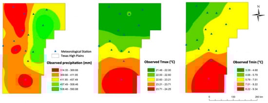
Figure 2.
Observed average annual precipitation (mm), maximum air temperature (°C), and minimum air temperature (°C) from 2000 to 2009.
In a previous study, the TXHPET network was used to evaluate the quality of the existing National Oceanic and Atmospheric Administration-National Centers for Environmental Information (NOAA-NCEI) climate data. The results found the quality of the publicly accessible NOAA-NCEI climate data is generally poor in the THP [26]. Also, there was an apparent lack of quality assurance/quality control (QA/QC) with the NOAA-NCEI datasets. The QA/QC methods, sensor information, or siting details were not available for the NOAA-NCEI climate data, and missing or unrealistic data were common [49]. Therefore, comparisons of closely located TXHPET and NOAA-NCEI stations showed differences for most weather parameters. Consequently, it was necessary to use the collected climate data from the research-grade, agro-meteorological stations as the control group to predict the future climatic change under the agricultural production system.
3.2. Comparisons of Observed, Raw GCM Simulated, and Bias-Corrected Climate Data
In this study, bias corrections were performed for 19 GCMs at each of the 14 agro-meteorological station locations. Since such a large amount of data were analyzed, the Halfway station and the GCM of access1-0 RCP 4.5 were selected to demonstrate the comparison of the observed, GCM simulated, and bias-corrected climate data. Results found a large bias between the observed and GCM simulated precipitation (Figure S1, Supplementary Materials). This suggested the bias correction was needed for this climate change study.
As for bias correction methods, initially, the commonly used quantile mapping method was used to correct the precipitation, maximum air temperature, and minimum air temperature. However, the quantile mapping method did not perform well with the precipitation data since a large mean difference existed between the GCM simulated and the observed precipitation collected by the research-grade agro-meteorological station (Figure S2). Therefore, the linear scaling method, which results in corrected data perfectly agreeing with the average monthly mean of the observed data, was selected to alter the GCM projected precipitation values. Results showed the bias-corrected precipitation from 2000 to 2009 using the linear scaling method had a better match with the monthly mean values of the TXHPET observations (Figure S2).
The bias-corrected average monthly (2000–2009) temperature data matched well with the historical measured data using the extensively utilized quantile mapping approach (Figure S3). This method not only corrected the mean values of temperatures, but also corrected temperatures for their distribution, such as standard deviation and percentiles (Figure S3) [50]. In addition, this method retained the variability in raw GCM simulated data after bias correction [51,52,53]. Bias-corrected monthly GCM-simulated temperatures also agreed well with observed values over the time period of 2000–2009 (Figure S4).
3.3. Trends of Future Climate Change in the Texas High Plains
After the bias corrections, the maximum and minimum air temperatures were predicted to increase in the THP region in the future (Figure 3 and Figure 4) while the precipitation would decrease (Figure 5). The increase in average annual maximum air temperature ranged from 1.8–2.4 °C, 2.4–3.0 °C, 2.8–3.4 °C, and 5.8–6.8 °C under the 2050–2059 RCP 4.5, 2090–2099 RCP 4.5, 2050–2059 RCP 8.5, and 2090–2099 RCP 8.5 scenarios, respectively, compared to the historical (2000–2009) observed maximum air temperature. It is worth noting that at the end of the 21st century (2090–2099) under the severe CO2 emission scenario (RCP 8.5), the maximum air temperature could increase by 5.5–6.4 °C. Moreover, the northern region displayed a larger temperature increase as compared to the southern region (Figure 3), which might be attributed to the relatively lower observed maximum air temperature in the northern region during the historical period (Figure 2). Days that are hotter than usual can result in the shortening of the maturity period for existing crops. Reduction in maturity period could decrease the time duration of crop for solar radiation use and nutrient assimilation, which may adversely impact the final yield [14,15]. The hotter conditions can also increase the risk of drought and heat stress of the crops, increasing the risk of associated crop failure.
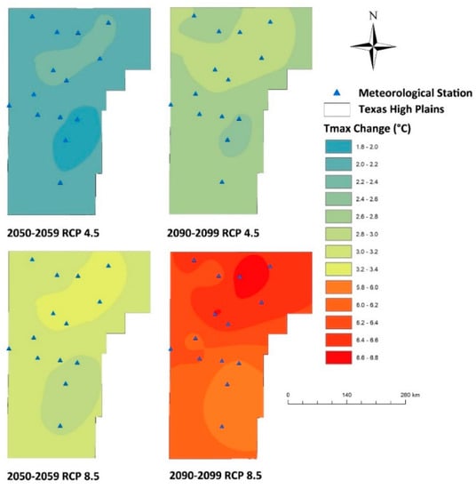
Figure 3.
Future changes in maximum air temperature (°C) compared to the historical (2000–2009) observed data.
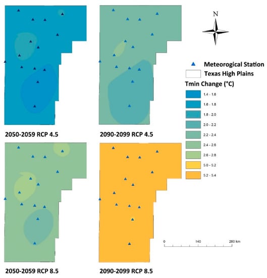
Figure 4.
Future changes in minimum air temperature (°C) compared to the historical (2000–2009) observed data.
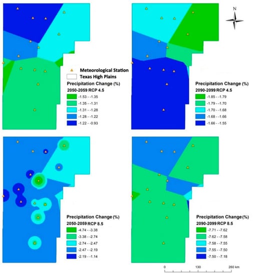
Figure 5.
Future changes in precipitation (%) compared to the historical (2000–2009) observed data.
The increase in average annual minimum air temperature varied from 1.4–2.0 °C, 2.0–2.4 °C, 2.2–2.8 °C, and 5.0–5.4 °C under the 2050–2059 RCP 4.5, 2090–2099 RCP 4.5, 2050–2059 RCP 8.5, and 2090–2099 RCP 8.5 scenarios, respectively, relative to the historical observed minimum air temperature (Figure 4). The increased amplitude of the minimum air temperature was lower than the maximum air temperature. It is interesting to find that at the end of the 21st century (2090–2099) under the severe CO2 emission scenario (RCP 8.5), the minimum air temperature would increase 4.5–5.5 °C uniformly across the entire THP (Figure 4).
The decrease in average annual precipitation shifted from 1.2–1.5%, 1.5–1.9%, 1.1–4.8%, and 7.1–7.7% under the 2050–2059 RCP 4.5, 2090–2099 RCP 4.5, 2050–2059 RCP 8.5, and 2090–2099 RCP 8.5 scenarios, respectively, relative to the historical observed precipitation (Figure 5). No consistent change pattern in the spatial distribution of precipitation was found between the RCPs and time periods in the THP. However, all the scenarios predicted a reduction of future precipitation, particularly by the end of the 21st century under the severe CO2 emission scenario (RCP 8.5), and precipitation could be reduced by approximately 7.5% in the THP (Figure 5). Since only 14 points (stations) across the Texas High Plains are available, the interpolation map may have relatively large uncertainty. However, this study mainly focuses on the relative changes to give an overview of the possible future climate change.
3.4. Uncertainty of the Future Climate Change in the Texas High Plains
Box plots of the climate data at each agro-meteorological station also showed an increase in average annual air temperatures and a decrease in average annual precipitation. Under the RCP 4.5 scenario, the average values of the precipitation reductions were within 5% for the 14 agro-meteorological stations in the middle (2050–2059) and the end (2090–2099) of the 21st century (Figure 6). The uncertainty of the precipitation change ranged from −30% to 55% and −35% to 35% under the 2050–2059 RCP 4.5 and 2090–2099 RCP 4.5 scenarios, respectively, according to 19 GCM projections. Under the RCP 8.5 scenario, the average values of the precipitation were reduced by 3% and 7% in the middle (2050–2059) and the end (2090–2099) of the 21st century, respectively (Figure 6). However, large uncertainties were found for the precipitation changes based on the 19 GCMs, which varied from −30% to 30% and −40% to 30% in the middle (2050–2059) and the end (2090–2099) of the 21st century, respectively. At Halfway, Modala et al. [20] found a 3–7% reduction in average annual precipitation according to three future climate models for the time period of 2041–2070 under the A2 climate scenario (high emission scenario) based on the CMIP3 simulations. However, our study found a change of precipitation from −26% to 29% with a model ensemble mean of −2.5% for a similar scenario according to 19 future climate models based on the CMIP5 simulations. Among the 19 GCMs, nine models predicted a reduction of future precipitation at the Halfway station.
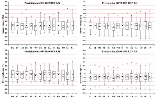
Figure 6.
Box plots of precipitation change (%) under the RCP 4.5 and 8.5 scenarios compared to the historical (2000–2009) observed data; DA, ET, MO, PE, BU, WT, WD, DI, FA, EA, HA, LO, LU, and LA indicate Dalhart, Etter, Morse, Perryton, Bushland, West Texas A&M University Feedlot, White Deer, Dimmitt, Farwell, Earth, Halfway, Lockney, Lubbock, and Lamesa.
As for air temperature, the maximum air temperature increased from −1 to 4 °C, 0 to 5 °C, 1 to 5 °C, and 4 to 10 °C under the 2050–2059 RCP 4.5, 2090–2099 RCP 4.5, 2050–2059 RCP 8.5, and 2090–2099 RCP 8.5 scenarios, respectively, according to 19 GCM predictions (Figure 7). The average values of maximum air temperature for those scenarios elevated ~2.0, 2.8, 3.0, and 6.5 °C. However, there is a large uncertainty depending on the GCM used, particularly for the severe emission scenario at the end of this century (Figure 7). All 19 GCMs projected an increase in the minimum air temperature in the future. The minimum air temperature could increase by 0 to 3 °C and 1 to 4.5 °C in the middle (2050–2059) and the end (2090–2099) of the 21st century under the RCP 4.5 scenario (Figure 8). A greater increase in minimum air temperature was identified under the RCP 8.5 scenario. Specifically, the air temperature increase shifted from 1.5 to 4.0 °C and 3.0 to 8.5 °C in the time periods of 2050–2059 and 2090–2099 using the 19 GCMs (Figure 8).
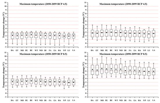
Figure 7.
Box plots of maximum air temperatures (°C) under the RCP 4.5 and 8.5 scenarios relative to the historical (2000–2009) observed data; DA, ET, MO, PE, BU, WT, WD, DI, FA, EA, HA, LO, LU, and LA indicate Dalhart, Etter, Morse, Perryton, Bushland, West Texas A&M University Feedlot, White Deer, Dimmitt, Farwell, Earth, Halfway, Lockney, Lubbock, and Lamesa.
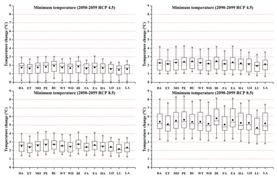
Figure 8.
Box plots of minimum air temperatures (°C) under the RCP 4.5 and 8.5 scenarios relative to the historical (2000–2009) observed data; DA, ET, MO, PE, BU, WT, WD, DI, FA, EA, HA, LO, LU, and LA indicate Dalhart, Etter, Morse, Perryton, Bushland, West Texas A&M University Feedlot, White Deer, Dimmitt, Farwell, Earth, Halfway, Lockney, Lubbock, and Lamesa.
4. Conclusions and Remarks
Climate change has the potential to affect water resources, agricultural production, and the well-being of people in general. The environment that provides us with water, food, air, habitat, and safety could be influenced by climate change and climate variability, especially when incurring weather extremes [54]. Given that the THP is a relatively hot and dry area comparatively, the forecasted increase in air temperatures and decrease in precipitation levels in the future could cause severe challenges in agricultural production and subsequently food security. This study showed a clear increase in future maximum and minimum air temperatures and a reduction in precipitation, particularly at the end of the 21st century with a severe CO2 emission scenario. The increase of temperature extremes and decrease in precipitation could induce the long-term drought or megadrought, which could affect agricultural land use, reduce crop yields, and increase crop prices [16,32]. An increasing drought problem can also impact the infrastructure and capacity of existing water systems, resulting in the compromised quantity and quality of irrigation and drinking water supplies, an increased risk of wildfires, dust storms, food insecurity, and human health concerns [55]. This study also indicated large uncertainties were found for the changes in precipitation and air temperatures based on the 19 GCMs. The uncertainty of the precipitation change ranged from −30% to 55%, −35% to 35%, −30% to 30%, and −40% to 30% under the 2050–2059 RCP 4.5, 2090–2099 RCP 4.5, 2050–2059 RCP 8.5, and 2090–2099 RCP 8.5 scenarios, respectively, according to 19 GCM projections. The maximum air temperature changed from −1 to 4 °C, 0 to 5 °C, 1 to 5, and 4 to 10 °C under the 2050–2059 RCP 4.5, 2090–2099 RCP 4.5, 2050–2059 RCP 8.5, and 2090–2099 RCP 8.5 scenarios, respectively, using 19 GCM predictions. Those values for the minimum air temperature were 0 to 3 °C, 1 to 4.5 °C, 1.5 to 4 °C, and 3 to 8.5 °C. This study demonstrated the uncertainty of the future climate analysis could be influenced by the selection of General Circulation Models and bias correction methods.
Supplementary Materials
The following is available online at https://www.mdpi.com/2071-1050/12/15/6036/s1. Figure S1: Statistical comparisons of average monthly (2000–2009) observed, access1-0 RCP 4.5 simulated, distribution mapping bias-corrected, and linear scaling bias-corrected precipitation at Halfway; obs_pcp_ovl, RCP4.5_P_ovl, RCP4.5_P_ovl_dm_hist, and RCP4.5_P_ovl_ls_hist indicate the observed, access1-0 RCP 4.5 simulated, distribution mapping bias-corrected, and linear scaling bias-corrected precipitation, respectively. Figure S2: Comparisons of monthly observed, access1-0 RCP 4.5 simulated, distribution mapping bias-corrected, and linear scaling bias-corrected precipitation during the time period of 2000–2009 at Halfway; obs_pcp_ovl, RCP4.5_P_ovl, RCP4.5_P_ovl_dm_hist, and RCP4.5_P_ovl_ls_hist indicate the observed, access1-0 RCP 4.5 simulated, distribution mapping bias-corrected, and linear scaling bias-corrected precipitation, respectively. Figure S3: Statistical comparisons of average monthly (2000–2009) observed, access1-0 RCP 4.5 simulated, and distribution mapping bias-corrected Tmax and Tmin at Halfway; obs_tmp_ovl_max, RCP4.5_T_ovl_max, RCP4.5_T_ovl_dm_hist_max, obs_tmp_ovl_min, RCP4.5_T_ovl_min, and RCP4.5_T_ovl_dm_hist_min indicate the observed, access1-0 RCP 4.5 simulated, and distribution mapping bias-corrected Tmax and Tmin. Figure S4: Comparisons of monthly observed, access1-0 RCP 4.5 simulated, and distribution mapping bias-corrected Tmax and Tmin during the time period of 2000-2009 at Halfway; obs_tmp_ovl_max, RCP4.5_T_ovl_max, RCP4.5_T_ovl_dm_hist_max, obs_tmp_ovl_min, RCP4.5_T_ovl_min, and RCP4.5_T_ovl_dm_hist_min indicate the observed, access1-0 RCP 4.5 simulated, and distribution mapping bias-corrected Tmax and Tmin.
Author Contributions
Conceptualization, Y.C., T.H.M., D.O.P., and G.W.M.; methodology, Y.C., G.W.M., J.E.M., and Q.W.; formal analysis, Y.C. and Q.W.; investigation, Y.C., T.H.M., and D.O.P.; resources, T.H.M., D.O.P., G.W.M., J.E.M., and D.K.B.; data curation, Y.C., Q.W., T.H.M., D.O.P., G.W.M., J.E.M., and K.R.H.; writing-original draft preparation, Y.C. and Q.W.; writing-review and editing, G.W.M., T.H.M., D.O.P., J.E.M., K.R.H., and D.K.B.; visualization, Q.W. and Y.C.; supervision, G.W.M., T.H.M., D.O.P., and D.K.B.; project administration, G.W.M., T.H.M., D.O.P., and D.K.B.; funding acquisition, G.W.M., T.H.M., D.O.P., and D.K.B. All authors have read and agreed to the published version of the manuscript.
Funding
This research was supported in part by the Ogallala Aquifer Program, a consortium between USDA-Agricultural Research Service, Kansas State University, Texas A&M AgriLife Research, Texas A&M AgriLife Extension Service, Texas Tech University, and West Texas A&M University. The TXHPET data sets used were acquired with funding support from the Ogallala Aquifer Program and grants from state and local water conservation agencies and commodity organizations. The data supported more than 20 Hatch projects.
Acknowledgments
We acknowledge the modeling groups, the Program for Climate Model Diagnosis and Intercomparison (PCMDI), and the World Climate Research Programme’s (WCRP’s) Working Group on Coupled Modelling (WGCM) for their roles in making available the WCRP CMIP3 and CMIP5 multi-model dataset. Support of this dataset is provided by the Office of Science, U.S. Department of Energy.
Conflicts of Interest
The authors declare no conflict of interest.
Appendix A
Box A1. Climate data pre-processing for meteorological stations maintained in accordance with the ASCE-EWRI specifications.
##### Select and organize observed climate data and change to SI unit
### Read in txt files and preserve:
### year, doy, maxT, minT, RH, SR, WS, precip
### List data from 2000/01/01 to 2009/12/31
### Yield one .txt file of the selected data
### Yield one .txt file for precipitation and one for temperature
# list the folder names for locating the data files
location <- c("BushlandDailyAll","DalhartDailyAll","DimmittDailyAll","EarthDailyAll","EtterDailyAll","FarwellDailyAll","HalfwayDailyAll","LamesaDailyAll","LockneyDailyAll","LubbockDailyAll","MorseDailyAll","PerrytonDailyAll","WhiteDeerDailyAll","WTDailyAll")
# set the path to read in txt
# (need to change this storage directory for further use)
path <- "~/Desktop/Historical_Climate_Data_Daily/"
setwd(path)
# set the path to save the files
save <- "~/Desktop/Observed_data/"
dir.create(save)
save_dir <- vector()
## Get the selected data files
for (i in 1:14) {
file <- paste(location[i],".txt",sep="")
tbl <- read.table(file,header=T,sep="\t",stringsAsFactors=F)
# extract the needed variables
tbl <- tbl[,c(3,4,18,20,27,42,47,50)]
# remove the row that shows NA from the variable "year"
for (ii in 1:nrow(tbl)) {
if (is.na(tbl[ii,1])) {
tbl <- tbl[-ii,]
}
}
# list the data from only 2000 to 2009;
# if the data start later than 2000 or end earlier than 2009
# then list from the true start date or list to the true end date
if (tbl[1,1]<2000) {
tbl <- tbl[which(tbl[,1]>=2000),]
}
if (tbl[nrow(tbl),1]>2009) {
tbl <- tbl[which(tbl[,1]<=2009),]
}
# create a new folder and save the selected table of data in it
save_dir[i] <- paste(save,location[i],sep="")
dir.create(save_dir[i])
save_i <- paste(save_dir[i],"/",file,sep="")
write.table(tbl,save_i,sep="\t",col.names=T,row.names=F)
}
## Get the pcp and tmp files
path2 <- "~/Desktop/Observed_data/"
for (ii in 1:14) {
sele_obs <- read.table(paste(save_dir[ii],"/",fname[ii],sep=""),header=T,sep="\t",stringsAsFactors=F)
# set the first day of the start year as the orgin to get the date from the variable "doy"
origin <- paste(as.character(sele_obs[1,1]),"/01/01",sep="")
origin_d <- as.Date(origin,"%Y/%m/%d")
# get the start date of data of this weather station
first_d <- as.Date(as.numeric(sele_obs[1,2])-1,origin=origin_d)
# convert the date to the format "YYYYMMDD"
# to use as the first line of the pcp and tmp files
startdate <- as.numeric(format(first_d,"%Y%m%d"))
pcp <- as.numeric(sele_obs[,8])
# convert the unit of pcp from (.01 in) to (mm)
pcp <- 0.254*pcp
# the tmp file would have both Tmax and Tmin data, seperated by ","
tmpmax <- as.numeric(sele_obs[,3])
tmpmin <- as.numeric(sele_obs[,4])
tmp <- as.data.frame(cbind(tmpmax,tmpmin))
# insert the first line (the start date)
pcp[2:(length(pcp)+1)] <- pcp[1:length(pcp)]
pcp[1] <- startdate
# write the data to the .txt files for pcp and tmp
tmp_file <- paste(save_dir[ii],"/obs_tmp.txt",sep="")
file.create(tmp_file)
writeLines(c(startdate,readLines(tmp_file)),tmp_file)
write.table(pcp,paste(save_dir[ii],"/obs_pcp.txt",sep=""),sep="",col.names=F,row.names=F)
write.table(tmp,tmp_file,sep=",",col.names=F,row.names=F,append=T)
}
Appendix B
Box A2. Compiling the projected future climate data obtained from the Downscaled Coupled Model Intercomparison Project Phase 5 (CMIP 5) Climate and Hydrology Projections.
##### Organize future climate data
### Read in csv files and preserve RCP4.5 and RCP8.5
### List data from 2000/01/01 to 2099/12/31
### Yield two .txt files for precipitation and two for temperature
# list the names of GCMs to locate the data files
sce19 <- c("access1-0.1","bcc-csm1-1.1","canesm2.1","ccsm4.1","cesm1-bgc.1","cnrm-cm5.1","csiro-mk3-6-0.1","gfdl-esm2g.1","gfdl-esm2m.1","inmcm4.1","ipsl-cm5a-lr.1","ipsl-cm5a-mr.1","miroc-esm-chem.1","miroc-esm.1","miroc5.1","mpi-esm-lr.1","mpi-esm-mr.1","mri-cgcm3.1","noresm1-m.1")
# set the path to read in csv
# (need to change this storage directory for further use)
path <- "~/Desktop/Future_Climate_Data/Bushland_19_GCMs/"
# To decide how many models the folder have
# if 19, extract the data of RCP4.5 and RCP8.5
if ("19" %in% strsplit(path,"_")[[1]]) {
for (ii in 1:19) {
wd <- paste(path,sce19[ii],sep="")
# set working directory
setwd(wd)
# paths to save the tidy data
save_45 <- paste(wd,"/RCP4.5",sep="")
save_85 <- paste(wd,"/RCP8.5",sep="")
# create folders to save the tidy data
dir.create(save_45)
dir.create(save_85)
## For precipitation
# read in the data
pr <- read.csv("pr.csv",header=F,sep=",",stringsAsFactors=FALSE)
# extract the data of RCP4.5 and RCP8.5
pr <- pr[,c(4,5)]
pr[,1:2] <- as.numeric(pr[,1:2])
# replace the NAs with 0
pr[which(is.na(pr[,1])),1] <- 0
pr[which(is.na(pr[,2])),2] <- 0
# add the first line: start date
pr[seq(2,nrow(pr)+1),] <- pr[seq(1,nrow(pr)),]
pr[1,] <- 20000101
write.table(pr[,1],paste(save_45,"/RCP4.5_P.txt",sep=""),sep="",col.names=FALSE,row.names=FALSE)
write.table(pr[,2],paste(save_85,"/RCP8.5_P.txt",sep=""),sep="",col.names=FALSE,row.names=FALSE)
## For temperature
# read in the data
tmin <- read.csv("tasmin.csv",header=F,sep=",",stringsAsFactors=FALSE)
tmax <- read.csv("tasmax.csv",header=F,sep=",",stringsAsFactors=FALSE)
# extract the data of RCP4.5 and RCP8.5
tmin <- tmin[,c(4,5)]
tmax <- tmax[,c(4,5)]
# convert the data to numbers to avoid some "data type" problems
tmin[,1:2] <- as.numeric(tmin[,1:2])
# replace the NAs with the data from the former line
tmin[which(is.na(tmin[,1])),1] <- tmin[which(is.na(tmin[,1]))-1,1]
tmin[which(is.na(tmin[,2])),2] <- tmin[which(is.na(tmin[,2]))-1,2]
tmax[,1:2] <- as.numeric(tmax[,1:2])
tmax[which(is.na(tmax[,1])),1] <- tmax[which(is.na(tmax[,1]))-1,1]
tmax[which(is.na(tmax[,2])),2] <- tmax[which(is.na(tmax[,2]))-1,2]
tem45 <- as.data.frame(cbind(tmax[,1],tmin[,1]))
tem85 <- as.data.frame(cbind(tmax[,2],tmin[,2]))
file_t45 <- paste(save_45,"/RCP4.5_T.txt",sep="")
file_t85 <- paste(save_85,"/RCP8.5_T.txt",sep="")
# create the empty files, in order to write in the first line
file.create(file_t45)
file.create(file_t85)
# add the first line: start date
writeLines(c(20000101,readLines(file_t45)),file_t45)
writeLines(c(20000101,readLines(file_t85)),file_t85)
write.table(tem45,file_t45,sep=",",col.names=F,row.names=F,append=T)
write.table(tem85,file_t85,sep=",",col.names=F,row.names=F,append=T)
}
}
Appendix C
Box A3. Linear scaling method for correcting 19 GCM projections.
##### Using Linear-scaling method to bias-correct precipitation
### need to use the package "hyfo"
# install.packages("hyfo")
# Load the package to this working environment
library(hyfo)
## Prepare the data files
# the first column should be Date
# list the folder names for locating the data files
stations <- c("Bushland_19_GCMs","Dalhart_19_GCMs","Dimmitt_19_GCMs","Earth_19_GCMs","Etter_19_GCMs","Farwell_19_GCMs","Halfway_19_GCMs","Lamesa_19_GCMs","Lockney_19_GCMs","Lubbock_19_GCMs","Morse_19_GCMs","Perryton_19_GCMs","WhiteDeer_19_GCMs","WT_19_GCMs")
# set the path to read in the data
# (need to change this storage directory for further use)
path <- "/Desktop/Future_Climate_Data/"
# do the loop for 14 weather stations
for (i in 1:14) {
loc <- strsplit(stations[i],"_")[[1]][1]
# do the loop for 19 models
for (ii in 1:19) {
# create the output folder and set it as current working directory
output <- paste0(path,stations[i],"/",sce19[ii],"/LinearScaling_biasCorrected")
dir.create(output)
setwd(output)
# input the observed data and projection data under RCP4.5 and RCP8.5
input_45 <- paste0(path,stations[i],"/",sce19[ii],"/","RCP4.5")
input_85 <- paste0(path,stations[i],"/",sce19[ii],"/","RCP8.5")
file_obs <- paste0(input_45,"/obs_pcp.txt")
file_45p <- paste0(input_45,"/RCP4.5_P.txt")
file_85p <- paste0(input_85,"/RCP8.5_P.txt")
obs_pcp <- read.table(file_obs,header=T)
startdate <- strsplit(colnames(obs_pcp),"X")[[1]][2]
colnames(obs_pcp) <- "obs"
# combine the RCP4.5 and RCP8.5 data into one table
frc_45p <- read.table(file_45p,header=T)
colnames(frc_45p) <- "pcp_45"
frc_85p <- read.table(file_85p,header=T)
colnames(frc_85p) <- "pcp_85"
obs_pcp <- cbind(obs_pcp,obs_pcp)
frc_pcp <- cbind(frc_45p,frc_85p)
# get the date of the precipitation data
obs_date <- seq.Date(from=as.Date(startdate,format="%Y%m%d"),by=1,length.out=nrow(obs_pcp))
frc_date <- seq.Date(from=as.Date("2000/01/01",format="%Y/%m/%d"),by=1,length.out=36525)
obs_pcp <- cbind(obs_date,obs_pcp)
frc_pcp <- cbind(frc_date,frc_pcp)
# add date as the first column
hdc_start <- as.numeric(obs_pcp[1,1]-frc_pcp[1,1])+1
hdc_end <- as.numeric(obs_pcp[1,1]-frc_pcp[1,1])+nrow(obs_pcp)
hdc_pcp <- frc_pcp[hdc_start:hdc_end,]
## Use Linear-scaling method to do bias correction
corrected_ls <- biasCorrect(frc_pcp,hdc_pcp,obs_pcp,preci=T)
ls_pcp <- corrected_ls[,c(2,3)]
ls_pcp[seq(2,nrow(ls_pcp)+1),] <- ls_pcp[seq(1,nrow(ls_pcp)),]
ls_pcp[1,] <- c(20000101,20000101)
# save the tables into text files
write.table(ls_pcp[,1],"RCP4.5_ls_P.txt",sep="",col.names=FALSE,row.names=FALSE)
write.table(ls_pcp[,2],"RCP8.5_ls_P.txt",sep="",col.names=FALSE,row.names=FALSE)
}
}
References
- Parry, M.L.; Rosenzweig, C.; Iglesias, A.; Livermore, M.; Fischer, G. Effects of climate change on global food production under SRES emissions and socio-economic scenarios. Glob. Environ. Chang. 2004, 14, 53–67. [Google Scholar] [CrossRef]
- Punkari, M.; Droogers, P.; Immerzeel, W.; Korhonen, N.; Lutz, A.; Venalainen, A. Climate Change and Sustainable Water Management in Central Asia; Asian Development Bank (ABD) Central and West Asia: Manila, Philippines, 2014. [Google Scholar]
- Bates, B.C.; Kundzewicz, Z.W.; Wu, S.; Palutikof, J.P. IPCC Technical Paper on Climate Change and Water; Cambridge University Press: Cambrige, UK, 2008. [Google Scholar]
- Intergovernmental Panel on Climate Change (IPCC). Climate change. Summary for Policy makers . In Climate Change 2007. The Physical Science Basis. Contribution of Working Group I to the Fourth Assessment Report of the Intergovernmental Panel on Climate; Solomon, S.D., Qin, M., Manning, Z., Chen, M., Marquis, K.B., Averyt, M., Tignor, H.L., Eds.; Cambridge University Press: Cambridge, UK, 2007. [Google Scholar]
- United States Environmental Protection Agency (USEPA). Climate Change: Basic Information. Available online: https://19january2017snapshot.epa.gov/climatechange/climate-change-basic-information_.html (accessed on 9 July 2020).
- Bourdages, L.; Huard, D. Climate Change Scenario over Ontario Based on the Canadian Regional Climate Model (CRCM4.2); Ouranos: Montreal, QU, Canada, 2010. [Google Scholar]
- Emami, F.; Koch, M. Modeling the Impact of Climate Change on Water Availability in the Zarrine River Basin and Inflow to the Boukan Dam, Iran. Climate 2019, 7, 51. [Google Scholar] [CrossRef]
- Henderson, B.; Cacho, O.J.; Thornton, P.; Van Wijk, M.; Herrero, M. The economic potential of residue management and fertilizer use to address climate change impacts on mixed smallholder farmers in Burkina Faso. Agric. Syst. 2018, 167, 195–205. [Google Scholar] [CrossRef]
- Shahvari, N.; Khalilian, S.; Mosavi, S.H.; Mortazavi, S.A. Assessing climate change impacts on water resources and crop yield: A case study of Varamin plain basin, Iran. Environ. Monit. Assess. 2019, 191, 134. [Google Scholar] [CrossRef] [PubMed]
- Fragoso, R.M.D.S.; Noéme, C.J.D.A. Economic effects of climate change on the Mediterranean’s irrigated agriculture. Sustain. Account. Manag. Policy J. 2018, 9, 118–138. [Google Scholar] [CrossRef]
- Weeks, J.B. High plains regional aquifer study. In Regional Aquifer-System Analysis Program of the US Geological Survey of Projects, 1978–1984; Sun, R.J., Ed.; US Government Printing Office: Washington, DC, USA, 1986. [Google Scholar]
- Allen, V.; Brown, C.; Segarra, E.; Green, C.; Wheeler, T.; Acosta-Martínez, V.; Zobeck, T. In search of sustainable agricultural systems for the Llano Estacado of the U.S. Southern High Plains. Agric. Ecosyst. Environ. 2008, 124, 3–12. [Google Scholar] [CrossRef]
- Webb, W.P. The Great Plains; Ginn and Co.: New York, NY, USA, 1931. [Google Scholar]
- Araya, A.; Kisekka, I.; Lin, X.; Prasad, P.V.; Gowda, P.; Rice, C.; Andales, A. Evaluating the impact of future climate change on irrigated maize production in Kansas. Clim. Risk Manag. 2017, 17, 139–154. [Google Scholar] [CrossRef]
- Cotterman, K.; Kendall, A.D.; Basso, B.; Hyndman, D.W. Groundwater depletion and climate change: Future prospects of crop production in the Central High Plains Aquifer. Clim. Chang. 2017, 146, 187–200. [Google Scholar] [CrossRef]
- Islama, A.; Ahuja, R.L.; Garciab, L.A.; Ma, L.; Saseendran, A.S.; Trout, T.J. Modeling the impacts of climate change on irrigated maize production in the Central Great Plains. Agric. Water Manag. 2012, 110, 94–108. [Google Scholar] [CrossRef]
- Bassu, S.; Brisson, N.; Durand, J.L.; Boote, K.; Lizaso, J.; Jones, J.W.; Rosenzweig, C.; Ruane, A.C.; Adam, M.; Baron, C.; et al. How do various maize crop models vary in their responses to climate change factors? Glob. Chang. Biol. 2014, 20, 2301–2320. [Google Scholar] [CrossRef]
- Crops and Plants. Available online: http://www.nass.usda.gov/ (accessed on 6 May 2013).
- Araya, A.; Hoogenboom, G.; Luedeling, E.; Hadgu, K.M.; Kisekka, I.; Martorano, L.G. Assessment of maize growth and yield using crop models under present and future climate in southwestern Ethiopia. Agric. For. Meteorol. 2015, 252–265. [Google Scholar] [CrossRef]
- Modala, N.R.; Ale, S.; Goldberg, D.W.; Olivares, M.; Munster, C.L.; Rajan, N.; Feagin, R.A. Climate change projections for the Texas High Plains and Rolling Plains. Theor. Appl. Clim. 2016, 129, 263–280. [Google Scholar] [CrossRef]
- Williams, A.A.; White, N.; Mushtaq, S.; Cockfield, G.; Power, B.; Kouadio, L. Quantifying the response of cotton production in eastern Australia to climate change. Clim. Chang. 2014, 129, 183–196. [Google Scholar] [CrossRef]
- Yang, M.; Xiao, W.; Zhao, Y.; Li, X.; Huang, Y.; Lü, F.; Hou, B.; Li, B. Assessment of Potential Climate Change Effects on the Rice Yield and Water Footprint in the Nanliujiang Catchment, China. Sustainability 2018, 10, 242. [Google Scholar] [CrossRef]
- Gharbia, S.; Gill, L.; Johnston, P.; Pilla, F. Multi-GCM ensembles performance for climate projection on a GIS platform. Model. Earth Syst. Environ. 2016, 2, 102. [Google Scholar] [CrossRef]
- Stewart, B.A.; Steiner, J.L. Water-use efficiency. In Dryland Agriculture: Strategies for Sustainability; Singh, R.P., Parr, J.F., Stewart, B.A., Eds.; Springer: New York, NY, USA, 1990; pp. 151–173. [Google Scholar]
- USDA-NRCS. The Soil Orders of Texas. Available online: https://www.nrcs.usda.gov/wps/portal/nrcs/detail/tx/home/?cid=nrcs144p2_003094 (accessed on 1 August 2019).
- Marek, T.H.; Porter, D.O.; Gowda, P.H.; Howell, T.A.; Moorhead, J.E. Assessment of Texas Evapotranspiration (ET) Networks, Final Report to the Texas Water Development Board for Contract. Available online: https://www.twdb.texas.gov/publications/reports/contracted_reports/doc/0903580904_evapotranspiration.pdf (accessed on 25 July 2020).
- Moorhead, J.E. Crop-Specific Drought Indices for Groundwater Management in the Texas High Plains, Master’s Thesis, West Texas A&M University, Canyon, TX, USA, 2012. [Google Scholar]
- American Society of Civil Engineers-Environmental & Water Resources Institute (ASCE-EWRI). The ASCE Standardized Reference Evapotranspiration Equation. Technical Committee report to the Environmental and Water Resources Institute of the American Society of Civil Engineers from the Task Committee on Standardization of Reference Evapotranspiration; ASCE-EWRI: Reston, VA, USA, 2005; p. 173. [Google Scholar]
- Reclamation. Downscaled CMIP3 and CMIP5 Climate Projections: Release of Downscaled CMIP5 Climate Projections, Comparison with Preceding Information, and Summary of User Needs. U.S. Department of the Interior, Bureau of Reclamation. Available online: http://gdo-dcp.ucllnl.org/downscaled_cmip_projections/techmemo/downscaled_climate.pdf (accessed on 5 August 2019).
- Bellamy, S.; Boyd, D.; Minshall, L. Determining the Effect of Climate Change on the Hydrology of the Grand River Watershed; Cambridge University Press: Cambridge, UK, 2002. [Google Scholar]
- Wu, Y.; Liu, S.; Gallant, A.L. Predicting impacts of increased CO2 and climate change on the water cycle and water quality in the semiarid James River Basin of the Midwestern USA. Sci. Total Environ. 2012, 430, 150–160. [Google Scholar] [CrossRef] [PubMed]
- Chen, Y.; Marek, G.W.; Marek, T.H.; Moorhead, J.E.; Heflin, K.R.; Brauer, D.K.; Gowda, P.; Srinivasan, R. Simulating the impacts of climate change on hydrology and crop production in the Northern High Plains of Texas using an improved SWAT model. Agric. Water Manag. 2019, 221, 13–24. [Google Scholar] [CrossRef]
- Riahi, K.; Grübler, A.; Nakićenović, N. Scenarios of long-term socio-economic and environmental development under climate stabilization. Technol. Forecast. Soc. Chang. 2007, 74, 887–935. [Google Scholar] [CrossRef]
- Clarke, L.E.; Edmonds, J.A.; Jacoby, H.D.; Pitcher, H.; Reilly, J.M.; Richels, R. Scenarios of Greenhouse Gas Emissions and Atmospheric Concentrations. Sub-Report 2.1a of Synthesis and Assessment Product 2.1; Climate Change Science Program and the Subcommittee on Global Change Research: Washington, DC, USA, 2007.
- Fujino, J.; Nair, R.; Kainuma, M.; Masui, T.; Matsuoka, Y. Multi-gas Mitigation Analysis on Stabilization Scenarios Using Aim Global Model. Energy J. 2006, 27, 343–354. [Google Scholar] [CrossRef]
- Hijioka, Y.; Matsuoka, Y.; Nishimoto, H.; Masui, T.; Kainuma, M. Global GHG emission scenarios under GHG concentration stabilization targets. J. Glob. Environ. Eng. 2008, 1, 97–108. [Google Scholar]
- Smith, S.J.; Wigley, T.M.L. Multi-Gas Forcing Stabilization with Minicam. Energy J. 2006, 27, 373–392. [Google Scholar] [CrossRef]
- Wise, M.; Calvin, K.; Thomson, A.; Clarke, L.; Bond-Lamberty, B.; Sands, R.; Smith, S.J.; Janetos, A.; Edmonds, J. Implications of Limiting CO2 Concentrations for Land Use and Energy. Science 2009, 324, 1183–1186. [Google Scholar] [CrossRef] [PubMed]
- Christensen, J.H.; Boberg, F.; Christensen, O.B.; Lucas-Picher, P. On the need for bias correction of regional climate change projections of temperature and precipitation. Geophys. Res. Lett. 2008, 35, 20709. [Google Scholar] [CrossRef]
- Teutschbein, C.; Seibert, J. Regional Climate Models for Hydrological Impact Studies at the Catchment Scale: A Review of Recent Modeling Strategies. Geogr. Compass 2010, 4, 834–860. [Google Scholar] [CrossRef]
- Teutschbein, C.; Seibert, J. Bias correction of regional climate model simulations for hydrological climate-change impact studies: Review and evaluation of different methods. J. Hydrol. 2012, 456, 12–29. [Google Scholar] [CrossRef]
- Varis, O.; Kajander, T.; Lemmela, R. Climate and Water: From Climate Models to Water Resources Management and Vice Versa. Clim. Chang. 2004, 66, 321–344. [Google Scholar] [CrossRef]
- Johnson, F.; Sharma, A. Accounting for interannual variability: A comparison of options for water resources climate change impact assessments. Water Resour. Res. 2011, 47, 04508. [Google Scholar] [CrossRef]
- Rojas, R.; Feyen, L.; Dosio, A.; Bavera, D. Improving pan-European hydrological simulation of extreme events through statistical bias correction of RCM-driven climate simulations. Hydrol. Earth Syst. Sci. 2011, 15, 2599–2620. [Google Scholar] [CrossRef]
- Sennikovs, J.; Bethers, U. Statistical downscaling method of regional climate model results for hydrological modelling. In 18th World IMACS Congress and MODSIM09 International Congress on Modelling and Simulation; Anderssen, R.S., Braddock, R.D., Newham, L.T.H., Eds.; Modelling and Simulation Society of Australia and New Zealand and International Association for Mathematics and Computers in Simulation: Cairns, Australia, 2009; pp. 3962–3968. [Google Scholar]
- Sun, F.; Roderick, M.L.; Lim, W.H.; Farquhar, G.D. Hydroclimatic projections for the Murray-Darling Basin based on an ensemble derived from Intergovernmental Panel on Climate Change AR4 climate models. Water Resour. Res. 2011, 47. [Google Scholar] [CrossRef]
- Lenderink, G.; Buishand, A.; Van Deursen, W. Estimates of future discharges of the river Rhine using two scenario methodologies: Direct versus delta approach. Hydrol. Earth Syst. Sci. 2007, 11, 1145–1159. [Google Scholar] [CrossRef]
- Rathjens, H.; Bieger, K.; Srinivasan, R.; Chaubey, I.; Arnold, J.G. CMhyd User Manual. Available online: https://swat.tamu.edu/media/115265/bias_cor_man.pdf (accessed on 1 August 2019).
- Holman, D.; Sridharan, M.; Gowda, P.; Porter, D.; Marek, T.; Howell, T.; Moorhead, J. Gaussian process models for reference ET estimation from alternative meteorological data sources. J. Hydrol. 2014, 517, 28–35. [Google Scholar] [CrossRef]
- Lafon, T.; Dadson, S.; Buys, G.; Prudhomme, C. Bias correction of daily precipitation simulated by a regional climate model: A comparison of methods. Int. J. Clim. 2012, 33, 1367–1381. [Google Scholar] [CrossRef]
- Ines, A.V.M.; Hansen, J. Bias correction of daily GCM rainfall for crop simulation studies. Agric. For. Meteorol. 2006, 138, 44–53. [Google Scholar] [CrossRef]
- Block, P.J.; Filho, F.D.A.S.; Sun, L.; Kwon, H.-H. A Streamflow Forecasting Framework using Multiple Climate and Hydrological Models. Jawra J. Am. Water Resour. Assoc. 2009, 45, 828–843. [Google Scholar] [CrossRef]
- Teutschbein, C.; Seibert, J. Is bias correction of regional climate model (RCM) simulations possible for non-stationary conditions? Hydrol. Earth Syst. Sci. 2013, 17, 5061–5077. [Google Scholar] [CrossRef]
- Crimmins, A.; Balbus, J.; Gamble, J.; Beard, C.; Bell, J.; Dodgen, D.; Eisen, R.; Fann, N.; Hawkins, M.; Herring, S.; et al. The Impacts of Climate Change on Human Health in the United States: A Scientific Assessment; U.S. Global Change Research Program: Washington, DC, USA, 2016; p. 312.
- Centers for Disease Control and Prevention U.S. Environmental Protection Agency National Oceanic; Atmospheric Agency American Water Works Association. When Every Drop Counts: Protecting Public Health during Drought Conditions—A Guide for Public Health Professionals; U.S. Department of Health and Human Services: Atlanta, GA, USA, 2010.


© 2020 by the authors. Licensee MDPI, Basel, Switzerland. This article is an open access article distributed under the terms and conditions of the Creative Commons Attribution (CC BY) license (http://creativecommons.org/licenses/by/4.0/).