Abstract
The rapid growth of air travel and aviation emissions in recent years has contributed to an increase in climate impact. Contrails have been considered one of the main factors of the aviation-induced climate impact. This paper deals with the formation of persistent contrails and its relationship with fuel consumption and flight time when flight altitude and true airspeed vary. Detailed contrail formation conditions pertaining to altitude, relative humidity and temperature are formulated according to the Schmidt–Appleman criterion. Building on the contrail formation model, the proposed model would minimise total travel time, fuel consumption and contrail length associated with a given flight. Empirical data (including pressure, temperature, relative humidity, etc.) collected from seven flight information regions in Chinese observation stations were used to analyse the spatial and temporal distributions of the persistent contrail formation area. The trade-off between flight time, fuel consumption and contrail length are illustrated with a real-world case. The results provided a valuable benchmark for flight route planning with environmental, flight time, sustainable flight trajectory planning and fuel consumption considerations, and showed significant contrail length reduction through an optimal selection of altitude and true airspeed.
1. Introduction
With the number of commercial aircraft increasing by 131% between 1990 and 2010, the civil aviation industry experienced a rapid growth in terms of passenger demand [1,2,3]. The growth of air transportation is expected to rise at 4.4% per annum in the next 20 years [4,5]. Such intensified air traffic comes at the expense of significant energy consumption and negative environmental impact [6,7,8,9]. This rapid growth has also contributed to an increase in pollution, which affects public health [10] as well as global climate change. However, due to the outbreak of COVID-19 in China, massive lockdowns were implemented to reduce the spread of the epidemic, which has caused tremendous impacts on people’s life around the world, including travel restrictions, curfews and quarantines. Therefore, there was a significant decrease in the number of flights and passengers. More and more industries are returning to normal operations, with the control of COVID-19. The Intergovernmental Panel on Climate Change established the flight operation evaluation system, which revealed that the aviation sector contributed to approximately 2% of the total anthropogenic carbon dioxide (CO2) emissions. These emissions are expected to grow at 3–4% per year [11]. In 2017, the International Civil Aviation Organisation Council (ICAO) adopted the world’s first global design certification standard governing aircraft CO2 emissions, which could also be taken as a measure of cruise fuel efficiency [12]. Aviation contributes to 5% of the global climate change when including the non-CO2 effects [13]. The emissions change the atmospheric composition in different ways [14]. For instance, NOX reacts with greenhouse gases methane (CH4) and ozone (O3) to deteriorate atmosphere chemistry [15], thereby changing the global radiative forcing. Further causes to the unbalanced earth radiation are attributed to aerosols and their precursors and contrails [16,17]. One of the most remarkable impacts is the increase in the average temperature of the earth [18]. Among the many means of transportation, such as air, railway, road and water transport, emissions from air transportation demonstrated the highest increasing rate. Reducing aviation emissions may be an efficient climate policy [19]. In order to highlight the significance of climate and address climate problems related to aviation, events as the “Paris Climate Change Conference” and “ICAO Global Aviation Dialogues on market-based measures to address climate change” were held during the 2013–2016 triennium.
Though emissions from aircraft engines are similar to other emissions resulting from fossil fuel combustion, they are unusual, as they are emitted at a high altitude (the upper troposphere and the lower stratosphere). These emissions are important environmental concerns, as a result of their global impact on climate change. The impacts of aviation include CO2 effects and non-CO2 effects ranging from NOx and water vapour to contrails and aerosols. While CO2 and water vapour are direct greenhouse gases, NOx emissions influence the atmospheric composition via chemical processes by depleting methane (cooling effects) and forming ozone (warming effects) [20].
The significance of the aforementioned individual effect on the overall climate change has been studied thoroughly by climate scientists [13] and quantified in the form of Radiative Forcing (RF) change [20,21]. A transport carbon footprint methodology has been proposed to identify unit carbon footprints [22]. An example can be found in Figure 1, from which we can observe that the CO2 emission shares were less than 50% of the total aviation radiative forcing when non-CO2 effects were considered. Furthermore, contrails were the most significant non-CO2 contributors, with considerable uncertainty due to the lack of scientific understanding.
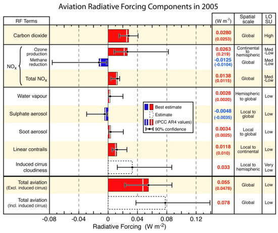
Figure 1.
Radiative forcing components from global aviation as evaluated from preindustrial times until 2005 [13].
According to the Schmidt–Appleman criterion, contrails are formed when the warm and moist exhaust gas of the engine is mixed with the cold ambient air under certain conditions [23,24]. The physical mechanism of contrail formation is relatively well understood [25]: Contrails are aircraft-induced cirrus clouds, which may persist and grow larger with air supersaturated with ice, and warm the atmosphere [26,27,28]. Contrails affect the earth’s radiation balance by trapping outgoing longwave radiations emitted by the earth and the atmosphere (positive radiative forcing) at a greater rate by reflecting incoming solar radiation (negative radiative forcing), thereby effectively increasing the global temperature. The influence of contrails is expected to become significant by 2050 [25]. Studies indicate that the environmental impact from persistent contrails is expected to be three to four times [29] or even ten times [28] greater than direct aviation-induced emissions.
There are two major reasons why contrails need to be avoided. Firstly, from a military perspective, even a short non-persistent contrail can be detected, which is particularly problematic for spy planes. Second, contrails have an impact on the climate because their warming effects are much greater than those caused by the CO2 from aircraft engines. This paper is only concerned with the persistent contrails, as short contrails have no real effect on the climate. The areas where persistent contrails can be formed are called Persistent Contrail Formation Areas (PCFA). Persistent contrails can only be formed when the aircraft flies into the airspace, the Schmidt–Appleman criterion [23,24] is met and the atmosphere is humid enough [30]. Contrails can be divided into aerodynamic contrails and combustion contrails; the former are caused by intense adiabatic cooling in the airflow over aircraft wings and behind the propeller blades [31] and are independent of the Schmidt–Appleman criterion and the exhaust properties [32], while the latter result from the engine exhaust gas. The effect of contrails on climate cannot be ignored [26,28,33]. In order to reduce the climate impact of contrails, various operational strategies such as reducing the flight altitude [34], implementing flexible operational measures [35] and shifting flight times to daylight hours [36] have been proposed. On the technological side, the use of alternative fuels [37] or kerosene with additives has received many commendations. However, it is suggested that fuel additives are not particularly effective in avoiding contrails [38].
Literature about mitigating aviation-induced contrails revealed that several simulation tools were used to analyse the vertical displacement of flight paths to avoid PCFA [5,34,39,40,41,42]. Research indicated that the aircraft could change the flight altitude or re-route to reduce contrail formation [30,31,32,35,43]. In 2011, a novel optimal control approach was presented to adjust aircraft flight paths for minimising contrail-inclusive flying cost [44]. Although these measures reduce contrails to a large extent, additional fuel consumption is still very expensive. A reduction in contrail distance can also cause an increase in flight time [45].
The flight profile is composed of three phases, namely climb, cruise and descent. In addition to these three phases, aircraft taxiing also results in carbon emissions. An element-by-element approach was developed in order to compute the environmental effects produced by each elementary source of pollution [46]. With regard to flight time and fuel consumption, the staple segment was cruise [47,48,49]. The optimal flight trajectories in the cruise stage are determined based on fuel consumption, flight time, CO2 emission and contrail formation [50,51,52]. However, as the amount of CO2 emission is proportional to fuel consumption [7,53,54], this paper only considers fuel consumption as a factor instead of CO2. The quantity of passengers is currently increasing sharply, and more jumbo jets have begun appearing in commercial civil aviation [14]. Apart from fuel consumption, flight time is also a necessary factor [55].
In this paper, we develop a flight trajectory planning and optimisation model aimed at minimising a combination of performance indicators including flight time, fuel consumption and environmental impact in terms of a contrail. A multi-objective mathematical optimisation problem is proposed, based on which the potential trade-off between several performance indicators is analysed in detail. The Pareto frontier in multi-objective functions corresponded to the different assignments of the weighted coefficient. The proposed contrail model and trajectory optimisation framework have the following features/contributions:
- Based on empirical data collected from Chinese observation stations and contrail models reported in the review of literature, a new framework for analysing the probability of contrail formation at distinct geographical locations and altitudes is presented.
- The optimisation problem proposed in this paper seeks a balance between flight time, fuel consumption and contrail length, by quantitatively analysing their trade-off. The optimisation framework allows decision-makers to trade off different objectives to cope with scenarios oriented towards specific stakeholders.
- Empirical data from China were used to estimate the probability of contrail formation and compare the results across different geographic locations and months. The results showed a significant variation of the contrail formation by area and season. Such findings suggest a great potential for flight trajectory optimisation, which was established by the realistic estimation of contrail formation.
The rest of the paper is organised as follows: In Section 2, we present the main model, which includes the contrail formation model, the speed and flying time models and the fuel consumption model. Section 3 presents the multi-objective optimisation problem. In Section 4, we explain a comprehensive case study and find the optimal flight altitude under different scenarios. Discussions are reported in Section 5. Finally, Section 6 provides some concluding remarks.
2. Contrail and Fuel Consumption Models
2.1. Contrail Formation Model
A contrail, which can be observed from the ground and in space, is formed when the hot and moist exhaust gas of an engine is mixed with the surrounding cold air during the flight. It has been confirmed that conditions such as temperature, pressure and relative humidity are relevant for the formation of a contrail, for which the sounding stations can provide essential information.
According to the Schmidt–Appleman criterion, contrails form only when the relative humidity (to water), denoted as , is above a threshold value [23,24,56]. One distinction needs to be made regarding , where the cloud is formed. This situation is excluded. When the relative humidity (to ice), , is equal or above 100%, contrails tend to persist [57]. Based on these factors, this paper considers the condition for contrail formation to be [30,58], as shown in Equations (1)–(5):
The threshold value can be expressed in terms of temperature (in degrees Celsius) as:
where is the saturation vapour pressure over water at a given temperature, which can be obtained by the Magnus formula [59]; (=1.25) is the emission index of water vapour; (=1004 )) represents the isobaric heat capacity of air; (in Pascal) is the ambient air pressure; (=0.6222) is the ratio of the molecular masses of water and dry air; (=43 × 106 J/kg) is the specific heat combustion; and (=0.15) is the average propulsion efficiency of the jet engine.
The relative humidity to ice is calculated using the Equation (6) [60]:
The flight altitude, which is one of the decision variables of the optimisation problem, is discretised and indexed as , where and represent the lowest and highest altitudes, respectively. Additionally, a flight path consists of multiple legs, indexed as in the direction of travel. The length of the leg is denoted by (in km), whereas the persistent contrail formation distance at altitude along the leg is denoted by , . The persistent contrail formation distances were determined as follows. First, the contrail formation condition is applied to the empirical data collected from the sounding stations, which leads to the spatial distribution of the PCFA.
Given the flight leg and discrete flying altitude , the corresponding atmospheric conditions (relative humidity, temperature, saturation vapour pressure) are identified based on the data collected from the sounding stations. Based on the Schmidt–Appleman criterion, we can then calculate which portion of the flight leg meets the criterion and hence allows a contrail, , to persist.
2.2. Speed and Flying Time Models
Wind direction and strength play important roles in the aircraft’s direction of travel, ground speed and fuel consumption. Due to the influence of crosswinds—both headwind and tailwind—the magnetic track deviates from the magnetic heading. In response, the aircraft adopts a drift angle to ensure that the magnetic track is aligned with the magnetic course. A two-dimensional Euclidean plane is considered to represent the vector pace for the wind model. For any leg at altitude , the true airspeed vector (in km/h) is denoted by , and the wind vector (in km/h) is . The ground speed vector (in km/h) is expressed as . The ground speed (in km/h) can then be expressed as . The flying time along the leg at altitude , assuming the wind speed and true airspeed (TAS) are relatively uniform, is expressed as (in h).
2.3. Fuel Consumption Model
The Base of Aircraft Data (BADA) is essential for calculating fuel consumption [61]. We focussed on a given flight in leg at altitude . Evidently, the fuel consumption under various conditions depended on the aircraft type ; however, for notation convenience, we omitted the dependence on , noting that all the parameters introduced below may be calibrated for each type of aircraft. For the jet and turboprop engines, the thrust-specific fuel consumption, (in kg/(min·kN)), is a function of the (in knots), which is a scalar. The following Equations (7)–(9) are adapted from [61].
where constants and are available from BADA and depend on the aircraft type. The nominal fuel flow, (in kg/min), can be calculated based on the thrust, (in N), which also depends on the TAS implicitly:
Accordingly, the fuel consumption for the entire leg at altitude is defined as (in kg):
where (in h) is the flying time obtained from Section 2.2.
3. Multi-Objective Optimisation Problem
An aircraft can change the flight altitude to avoid PCFA and heading to accommodate crosswind. These are, however, constrained by the aircraft’s manoeuvrability and the air traffic controls. These constraints are either explicitly incorporated in the model, or implicitly in the empirical dataset presented in Section 4. This section presents the complete multi-objective optimisation problem, including variables, objectives and constraints.
3.1. Variables and Parameters
The proposed optimisation problem requires the optimal choices of flying altitude and true airspeed to be adopted by a given flight, in order to minimise the contrail formation, flying time and fuel consumption. This is a mixed discrete-continuous problem, in the sense that we only consider a finite number of altitudes to be allowed by regulations, while treating the true airspeed as a continuous decision variable within a proper range.
| Index of flight altitude | |
| Index of flight leg | |
| Altitude (indexed by ) of flight cruising in leg | |
| True airspeed of the flight cruising in leg at altitude . |
3.2. Objective Function
When the aircraft is cruising in a certain leg at altitude , the ground speed, which is jointly determined by the wind speed and true airspeed (TAS), affects the flight time. Conversely, fuel consumption in the same leg depends on the TAS and flight time. Therefore, when the true airspeed varies between the minimum and maximum allowable speeds, the flight time and fuel consumption also change and may reach their respective minima at distinct true airspeeds. Therefore, the problem of minimising contrails with additional consideration for fuel burn and flying time is shown in Equation (10) as a multi-objective optimisation problem:
where and are weights used to indicate the relative importance of individual objectives in the overall optimisation. In the above expression, we calculate that
where , , and are defined in Section 2.1, Section 2.2 and Section 2.3, respectively. In the Equation (10), we normalise the three individual objectives using Equations (14)–(16):
3.3. Constraints
We impose the following constraints on the optimisation problem, as shown in Equations (17)–(20):
Equation (18) stipulates that only one such altitude choice can be adopted for each leg; Equation (17) expresses the discrete altitude choices for each leg; Equation (19) provides the set of feasible altitude values; and Equation (20) specifies the feasible true airspeed range, which is obtained from empirical data.
3.4. Solution Method
The proposed optimisation problem is a non-linear and non-convex mixed-integer programme. The number of integer decision variables is M × N. In a typical application scenario (see Section 4), both the numbers of legs and feasible flying altitudes are limited. Therefore, the problem can be decomposed into independent continuous optimisation problems, where the Complete Enumeration Method is used to solve the proposed problem. Alternatively, for larger and more complex optimisation scenarios, heuristics [62,63] may be employed.
4. Case Study
4.1. Seven Flight Information Regions in China Document Text
There are nearly 100 sounding stations in China available for gathering meteorological data, which are only observed twice a day, at 00Z and 12Z. Specifically, there were observations in May. Radio soundings in 2014 were used for the case study. The data were collected from seven Flight Information Regions (FIRs), namely Beijing (ZBAA), Urumqi (ZWWW), Shenyang (ZYYY), Shanghai (ZSSS), Kunming (ZPPP), Lanzhou (Yuzhong) and Guangzhou (Qingyuan). We counted the number of instances per month where persistent contrail formation conditions were satisfied (see Section 2.1), and the results are shown in Figure 2. Overall, the data showed that persistent contrails were less likely to form in the southern parts of China (Guangzhou, Kunming). It also revealed that persistent contrails were most prevalent in the winter and early spring and were the least seen during the summer [64]. However, the data suggested that there was an obvious seasonal variation in Guangzhou and Kunming, and that the contrails were concentrated in June, July and August, rather than winter or early spring. This may be due to low relative humidity during winter or early spring, and high relative humidity in June, July and August. Additionally, no discernible seasonal variations could be characterised for the other five regions.
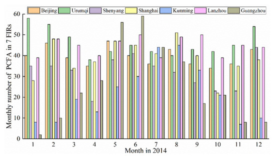
Figure 2.
Monthly numbers of persistent contrail formation areas (PCFA) in 2014 in 7 flight information regions (FIRs). The different FIRs are denoted by various colours.
4.2. Altitude and Thickness of PCFA
The radio soundings data from Nanjing in 2014 were used as an example to calculate the thickness of PCFA. The thickness at a given location is defined as the maximum vertical interval (unit in metre) in which the persistent contrail formation conditions are met. The empirical distribution of the PCFA’s thickness is shown in Figure 3. The relative probability of PCFA thickness was 22.59% (300 m), 12.93% (600 m), 9.52% (900 m) and 5.03% (1200 m), as shown in the black squares. The blue stars show that there was a high probability (over 50%) (red line) for a PCFA thickness not exceeding 1200 m, which proves that it is possible for an aircraft to change its flight altitude to avoid PCFA.
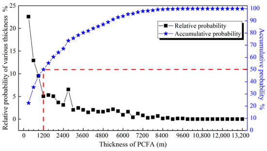
Figure 3.
Thickness proportion in Nanjing, 2014.
The black squares represent the relative probability of the PCFA’s thickness, whereas the blue stars represent the accumulative probability of PCFA’s thickness.
The Kolmogorov–Smirnov test was used to check the distribution of PCFA altitude against the normal distribution. The results revealed a significance level of 0.082, which is greater than 0.05. Therefore, it was concluded that the relative frequency of PCFA at each altitude can be characterised to follow the normal distribution. Figure 4 shows the empirical PCFA distribution.
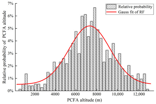
Figure 4.
PCFA altitude distribution. The relative probabilities of PCFA altitude from 6000 to 8000 m are generally over 5%. However, this probability function shows that the PCFA altitude is less at a higher altitude (>11,000 m) and at a lower altitude (<3000 m).
We evaluated the effect of changing flight altitude on the probability of avoiding PCFA, as shown in Figure 5. For example, if an aircraft is cruising at an altitude of 10,100 m (initial flight altitude), climbing 600 m (to 10,700 m) results in a 14.86% probability of avoiding PCFA, while the probability increases to 25.68% by climbing 1200 m (to 11,300 m). These empirical results motivate the adaptive adjustment of the flight altitude in order to avoid PCFA and serve as the basis for further investigation of the formation of contrail areas.
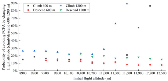
Figure 5.
Probability of avoiding PCFA by changing flight altitude.
4.3. Spatial Distribution of PCFA
Based on the meteorological data collected at the individual sounding stations (e.g., pressure, wind speed, wind degree, temperature and relative humidity), we may infer the meteorological conditions between the stations using spatial interpolation and compute the spatial distribution of PCFA using the formulae in Section 2.1. As an example, we considered a flight path from ZWWW (Urumqi) to ZSSS (Shanghai), with a distance of 3439 km (from waypoint URC to waypoint PK) in an A319 aircraft with a mass of 60,000 kg. Figure 6 shows the waypoints along this flight path represented by yellow dots.
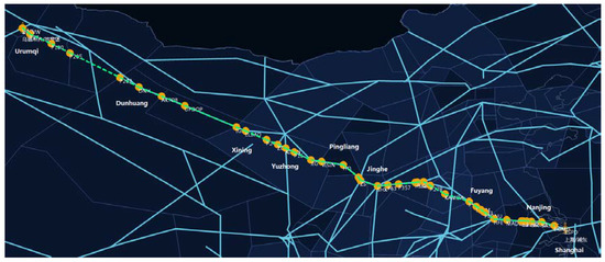
Figure 6.
Flight path from ZWWW (Urumqi) to ZSSS (Shanghai). The meteorological data are from sounding stations labelled as Urimqi, Dunhuang, Xining, etc. The aircraft should fly along the green line from ZWWW to ZSSS.
According to the Filed Flight Plan message (FPL), the cruising altitude was 10,700 m, and a higher altitude was not considered a result of the aircraft performance, control regulations and operational safety. In this example, we only focussed on flight altitudes ranging from 7500 m to 10,700 m with an increment of 600 m (i.e., ). We only considered the cruising phase above 7500 m, not the initial climb and final descent phases. The sounding stations relevant to the flight path were Urumqi (ID: 51463), Dunhuang (ID: 52418), Xining (ID: 52866), Yuzhong (ID: 52983), Pingliang (ID: 53915), Jinghe (ID: 57131), Fuyang (ID: 58203), Nanjing (ID: 58238) and Shanghai (ID: 58362). As these sounding observation stations were discrete, relevant data such as pressure, relative humidity and temperature between two stations were available only by linear interpolation. We used the data collected on 9 December 2014 to calculate the spatial distribution of PCFA along the flight path in accordance to the Schmidt–Appleman criterion. The result is shown in Figure 7, where the dark areas indicate the PCFA.
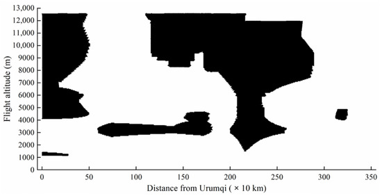
Figure 7.
Spatial distribution of PCFA. When the aircraft flew in the dark area, contrails were formed; contrail length is equal to flight distance.
In the following sections, we present the optimisation results that simultaneously minimised total travel time, fuel consumption and contrail length. As an additional input data of the model, the wind directions and speeds along the flight path of interest are shown in Figure 8. In this figure, the flight path was divided into eight spatial legs, where the wind direction and speed in each leg at a certain altitude (7500 m, 8100 m, 8900 m, 9500 m, 10,100 m, 10,700 m) is shown. The results reveal the predominant direction of the wind—West, largely due to the jet stream.
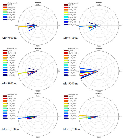
Figure 8.
Wind direction and speed in the 8 legs at 6 different altitudes.
Each sub-figure corresponds to an altitude. For example, at 7500 m, the wind directions (wind speeds) of eight different legs are 267.4° (47.3 kt), 266.3° (52.8 kt), 264.3° (71.2 kt), 259.6° (85.9 kt), 253.7° (58.2 kt), 237.3° (45.5 kt), 255.2° (38.6 kt) and 281.4° (34.2 kt), respectively.
4.4. Numerical Studies
4.4.1. Contrail Weight and Leg Number
Similar to the first case, we considered and , which meant that we did not consider contrail formation and instead focussed only on the trade-off between flying time and fuel consumption. Additionally, , which meant that the flying altitude and TAS were fixed throughout the cruising phase. The possible altitudes were 7500 m, 8100 m, 8900 m, 9500 m, 10,100 m and 10,700 m. As air density decreases and wind speed increases with the rise of flight altitude, the fuel consumption was the least at the highest level when TAS was the same. To ensure minimum fuel consumption, it was essential to choose the optimal TAS in each flight altitude, on the condition that the TAS meets the need of the flight envelope (see Figure 9); such a constraint has been reflected in (20).
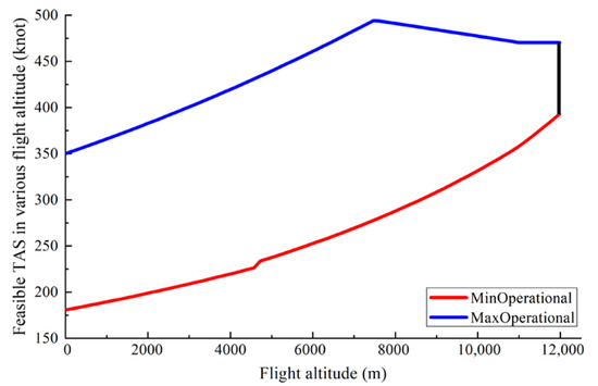
Figure 9.
Flight envelope constraints of A319. Aircraft operational speed has to meet the flight envelope constraints to ensure safety.
Figure 10 shows the trade-off between the flight time and fuel consumption, enabled by selecting different TAS for the cruising phase of the flight. At the same altitude, the flight time was a monotonically decreasing function of TAS. However, fuel consumption is a convex function of TAS with a unique minimum, which suggests the existence of a unique TAS. It also shows that increasing flying altitude tends to decrease both flight time and fuel consumption under the same TAS.
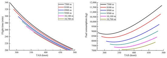
Figure 10.
At different flight altitudes, the relationship between true airspeed (TAS) and flight time (Left) and fuel consumption (Right).
Table 1 presents the trade-off between the flying time and fuel consumption in the optimal solution, where (fuel weight) varies from 0 to 1. Note that the optimal time and fuel consumption for is the same. The weight of flight time is higher than fuel consumption when ranges from 0.1 to 0.5, so the aircraft should fly at the maximum speed, but cannot exceed the maximum operating speed. The optimal TAS, denoted by the green stars, is shown in Figure 11 for a different fuel consumption weight .

Table 1.
The trade-off between fuel consumption and flight time in the optimal solution.
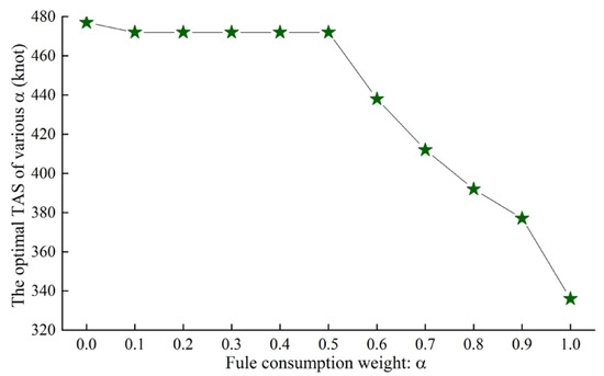
Figure 11.
Optimal TAS for minimum objective function. When , the optimal TAS is 477 knots, and when , it is 336 knots.
4.4.2. Leg Number
In this section, we considered multiple (8) flight legs in which the flying altitude and TAS were to be optimised. Figure 12 shows the optimal flying altitude, where the weight for contrail and the optimal altitude is insensitive to the weight . In Figure 13, the optimal flying altitudes are shown for and . Compared to Figure 12, the contrail formation in Figure 13 resulted in a flying altitude profile that avoided most of the PCFA.
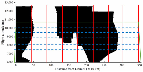
Figure 12.
Optimal altitude with The dark areas indicate PCFA; the optimal altitude is indicated as the solid green line.
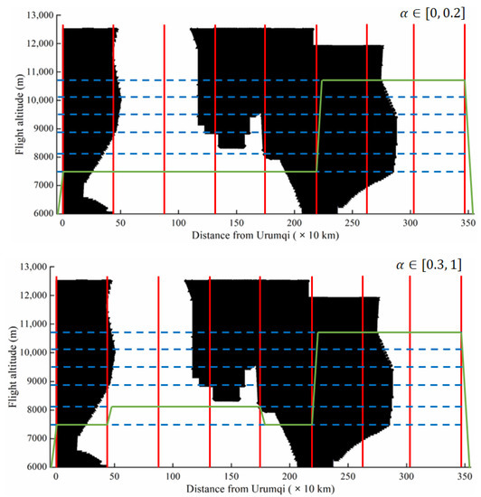
Figure 13.
Optimal altitude with and (Up) or (Down). Dark areas indicate PCFA; the optimal altitude is indicated as the solid green line. The optimal flight altitude remains constant for and , respectively.
Figure 14 shows the optimal TAS in different flight legs when different values of the weight were chosen. In most cases, the TAS underwent a drastic rise when the aircraft flew over leg 6. This is possibly caused by the change in the wind direction and speed. We also observed that the TAS increased with a decrease in (weight for fuel consumption), which is plausible as higher TAS requires higher engine thrust.
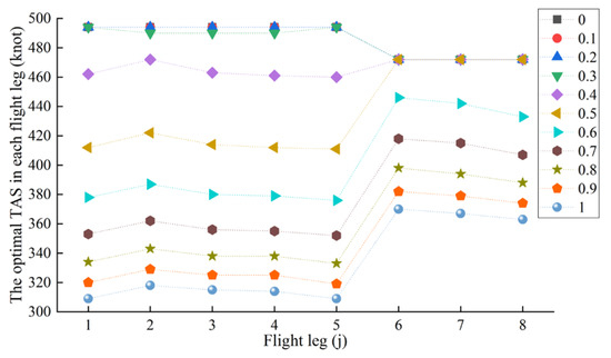
Figure 14.
Relationship between the weight and the optimal TAS in each leg.
We conducted a preliminary sensitivity analysis for (fuel consumption weight), as seen in Table 2. The contrail length was insensitive to the changes in when was set to 0 or 0.5, which suggested that a more subtle trade-off between a contrail and fuel/time may exist for ; this is further investigated in the next section. We also observed that the contrail length could be reduced by nearly half compared to the case, by assigning non-zero weight . However, this results in much higher fuel consumption, as an aircraft frequently lowers the altitude to avoid PCFA. Lastly, for a fixed , increasing the resulted in less fuel consumption and longer flight time.
Table 2.
Comparison of fuel consumption, flight time and contrail length with different choices of under two scenarios: and . When , contrail length is reduced by 47.8% with more fuel consumption (34.1%) and more flight time (2.9%).
4.4.3. Sensitivity Analysis
A more in-depth sensitivity analysis in terms of the trade-off among contrail length, fuel consumption and flight time was conducted. Figure 15 shows the three-dimensional frontier for the three-objective optimisation problem. The range of the weights is: . The objectives are relatively evenly traded off between flight time and fuel consumption. However, the objectives go through some abrupt changes along the “Contrail Length” axis (e.g., when varies), as indicated by the sparsity of the black stars along the “Contrail Length” axis. Such a distinction in the sensitivity with respect to different objectives is due to the irregular spatial distribution of the PCFA (see Figure 7).
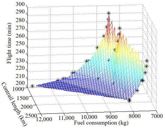
Figure 15.
The Pareto frontier for joint contrail-fuel-time optimisation. The optimal solutions corresponding to a different selection of the parameters are shown as black stars.
5. Discussion
In this case study, sounding station data in seven FIRs in 2014 were analytically quantified, showing higher possibilities of contrail formation in June and July in Kunming and Guangzhou, and in January, February and December in Urumqi. This could be a referential direction for changing flight altitude to avoid PCFA in different areas. Nanjing, located in the eastern part of China, is in the airport density centre. Results from 2014 showed that the thickness of PCFA less than 1200 m was about 50%, which served as the basis for changing flight altitude. Figure 7 demonstrates the 2-D spatial distribution of PCFA along a flight route. The wind speed and wind direction may be different in various positions; better use of wind can have a positive effect on the reduction in flight time and fuel consumption. When we do not consider the effect of contrails and set the flight leg as only one, with increasing , the optimal flight time decreases, while the optimal fuel consumption and TAS increase. The flight profile will have its ups and downs because of contrails. This increases the possibility of conflicts and the air traffic controllers’ workload. It is necessary to set a trade-off among different stakeholders.
Disruptive technology allows Air Traffic Control (ATC) to acquire the latest information about contrails and flight coordinates with low latency, to bring about a significant improvement of the quality of decision-making by adapting environment changes. Understanding the optimal flight trajectory in terms of fuel consumption and contrail avoidance can help reduce the regional aviation emission and achieve sustainable flight operations. The proposed method provides metrics and assessment mappings of a possible set of flight trajectories and suggests an optimal flight trajectory with the least impact on aviation emission that complies with the operating procedures from ATC perspectives. The decentralisation of trajectory optimisation improves the sustainable development of environmental flight operations and reaches successful sustainable aviation emission control in the ever-evolving perspective of global environmental change.
6. Conclusions
This paper focuses on contrail formation and its relationship with fuel consumption and flight time when flight altitude and true airspeed vary. Detailed contrail formation conditions pertaining to altitude, relative humidity and temperature were formulated according to the Schmidt– Appleman criterion. Building on the contrail formation model, we proposed a multi-objective optimisation problem that seeks to minimise the travel time, fuel consumption and contrail length associated with a given flight.
Empirical data collected from seven flight information regions in China were used to analyse the spatial and temporal distributions of the persistent contrail formation area. A case study of the proposed optimisation problem suggested, on a quantitative level, the trade-off between flight time, fuel consumption and contrail length. The optimisation results provided a valuable benchmark for flight route planning with environmental considerations, as they revealed that significant contrail length reduction can be achieved through an optimal selection of altitude and true airspeed.
This paper explores the multi-objective optimisation of flight speed and altitude to address environmental concerns pertaining to contrails. One should note that this research still has several limitations, which should be improved upon in future research. The frequent change of flight altitude increases the possibility of potential conflicts with other aircraft and increases the workload of ATCs and pilots to a large extent. Passengers also feel uncomfortable when they experience the ups and downs of an aircraft. The optimisation method proposed also needs to be improved with some heuristic algorithms to improve the optimal speed. To achieve uniformity in civil aviation, Air Traffic Management (ATM) authorities should propose some relevant measures and highlight the importance of collaborative decision making among passengers, ATCs, pilots and environmentalists.
Author Contributions
Conceptualization K.K.H.N. and L.-T.H.; Data curation D.X.; Formal analysis D.X.; Funding acquisition L.-T.H.; Investigation D.X. and L.-T.H.; Resources L.-T.H.; Supervision K.K.H.N. and L.-T.H.; Validation D.X.; Visualization D.X.; Writing—original draft D.X.; Writing—review & editing K.K.H.N. and L.-T.H. All authors have read and agreed to the published version of the manuscript.
Funding
This research received no external funding.
Acknowledgments
The research is supported by the Interdisciplinary Division of Aeronautical and Aviation Engineering, The Hong Kong Polytechnic University, Hong Kong SAR, Department of Land Surveying and Geo-Informatics, The Hong Kong Polytechnic University, Hong Kong SAR and the Department of Earth and Space Sciences, Southern University of Science and Technology, Shenzhen.
Conflicts of Interest
The authors declare that they have no known competing financial interest or personal relationship that could have appeared to influence the work reported in this paper.
References
- Huls, D. Current Market Outlook 2014–2033; Boeing Commercial Airplanes: Seattle, WA, USA, 2014. [Google Scholar]
- Airbus, S. Global Market Forecast-Flying on demand 2014–2033; Airbus SAS: Blagnac Cedex, France, 2014. [Google Scholar]
- Lee, C.K.M.; Ng, K.K.H.; Chan, H.K.; Choy, K.L.; Tai, W.C.; Choi, L.S. A multi-group analysis of social media engagement and loyalty constructs between full-service and low-cost carriers in Hong Kong. J. Air Transp. Manag. 2018, 73, 46–57. [Google Scholar] [CrossRef]
- Airbus, G.M.F. Growing Horizons 2017–2036; Airbus: Toulouse, France, 2017. [Google Scholar]
- Ng, K.K.H.; Lee, C.K.M.; Chan, F.T.S.; Lv, Y. Review on meta-heuristics approaches for airside operation research. Appl. Soft Comput. 2018, 66, 104–133. [Google Scholar] [CrossRef]
- Li, F.; Lee, C.-H.; Chen, C.-H.; Khoo, L.P. Hybrid data-driven vigilance model in traffic control center using eye-tracking data and context data. Adv. Eng. Inform. 2019, 42, 100940. [Google Scholar] [CrossRef]
- Li, F.; Chen, C.-H.; Xu, G.; Khoo, L.P.; Liu, Y. Proactive mental fatigue detection of traffic control operators using bagged trees and gaze-bin analysis. Adv. Eng. Inform. 2019, 42, 100987. [Google Scholar] [CrossRef]
- Du, S.; Razavi, S. Fault-tolerant control of variable speed limits for freeway work zone using likelihood estimation. Adv. Eng. Inform. 2020, 45, 101133. [Google Scholar] [CrossRef]
- Ng, K.K.H.; Lee, C.K.M.; Zhang, S.Z.; Wu, K.; Ho, W. A multiple colonies artificial bee colony algorithm for a capacitated vehicle routing problem and re-routing strategies under time-dependent traffic congestion. Comput. Ind. Eng. 2017, 109, 151–168. [Google Scholar] [CrossRef]
- Kampa, M.; Castanas, E. Human health effects of air pollution. Environ. Pollut. 2008, 151, 362–367. [Google Scholar] [CrossRef]
- International Civil Aviation Organization (ICAO). 2016 Environmental Report; ICAO Web: Hong Kong, China, 2016. [Google Scholar]
- Postorino, M.N.; Mantecchini, L. An Element-by-Element Approach for a Holistic Estimation of the Airport Carbon Footprint. In Sustainable Aviation; Springer: Berlin/Heidelberg, Germany, 2020; pp. 193–214. [Google Scholar]
- Lee, D.S.; Fahey, D.W.; Forster, P.M.; Newton, P.J.; Wit, R.C.N.; Lim, L.L.; Owen, B.; Sausen, R. Aviation and global climate change in the 21st century. Atmos. Environ. 2009, 43, 3520–3537. [Google Scholar] [CrossRef]
- Government of the United Kingdom. Royal Commission on Environmental Pollution Special report. In The Environmental Effects of Civil Aircraft in Flight; Royal Commission on Environmental Pollution: London, UK, 2003. [Google Scholar]
- Holmes, C.D.; Tang, Q.; Prather, M.J. Uncertainties in climate assessment for the case of aviation NO. Proc. Natl. Acad. Sci. USA 2011, 108, 10997–11002. [Google Scholar] [CrossRef]
- Lee, D.-S.; Gonzalez, L.F.; Walker, R.; Periaux, J.; Onate, E. Reduction environmental effects of civil aircraft through multi-objective flight plan optimisation. In IOP Conference Series: Materials Science and Engineering; IOP Publishing: Sydney, Australia, 2010; p. 012197. [Google Scholar]
- Köhler, M.O.; Rädel, G.; Shine, K.P.; Rogers, H.L.; Pyle, J.A. Latitudinal variation of the effect of aviation NOx emissions on atmospheric ozone and methane and related climate metrics. Atmos. Environ. 2013, 64, 1–9. [Google Scholar] [CrossRef]
- Baumgardner, D.; Miake-Lye, R.C.; Anderson, M.R.; Brown, R.C. An evaluation of the temperature, water vapor, and vertical velocity structure of aircraft contrails. J. Geophys. Res. Atmos. 1998, 103, 8727–8736. [Google Scholar] [CrossRef]
- Chow, S.Y.A. Aviation and city’s climate change policies: An analysis of emissions and emission inventory of Hong Kong. In Proceedings of the 16th International Conference of Hong Kong Society for Transportation Studies, Hong Kong, China, 17–20 December 2011. [Google Scholar]
- Lee, H.; Li, G.; Rai, A.; Chattopadhyay, A. Real-time anomaly detection framework using a support vector regression for the safety monitoring of commercial aircraft. Adv. Eng. Inform. 2020, 44, 101071. [Google Scholar] [CrossRef]
- Wee, H.J.; Lye, S.W.; Pinheiro, J.-P. An integrated highly synchronous, high resolution, real time eye tracking system for dynamic flight movement. Adv. Eng. Inform. 2019, 41, 100919. [Google Scholar] [CrossRef]
- Postorino, M.N.; Mantecchini, L. A transport carbon footprint methodology to assess airport carbon emissions. J. Air Transp. Manag. 2014, 37, 76–86. [Google Scholar] [CrossRef]
- Schmidt, E. Die entstehung von eisnebel aus den auspuffgasen von flugmotoren. Schr. Dtsch. Akad. Luftfahrtforsch. Verl. R. Oldenbourg München Heft 44 1941, 5, 1–15. [Google Scholar]
- Appleman, H. The formation of exhaust condensation trails by jet aircraft. Bull. Am. Meteorol. Soc. 1953, 34, 14–20. [Google Scholar] [CrossRef]
- Lim, Y.; Gardi, A.; Sabatini, R. Modelling and evaluation of aircraft contrails for 4-dimensional trajectory optimisation. SAE Int. J. Aerosp. 2015, 8, 1–12. [Google Scholar] [CrossRef]
- Schumann, U. Formation, properties and climatic effects of contrails. Comptes Rendus Phys. 2005, 6, 549–565. [Google Scholar] [CrossRef]
- Djojodihardjo, H. Climate change creativity for cirrus clouds and contrails control. In 2015 International Conference on Space Science and Communication (IconSpace); IEEE: Piscataway, NJ, USA, 2015; pp. 503–508. [Google Scholar]
- Mannstein, H.; Schumann, U. Aircraft induced contrail cirrus over Europe. Meteorol. Z. 2005, 14, 549–554. [Google Scholar] [CrossRef]
- Green, J. Air Travel-Greener by Design. Mitigating the environmental impact of aviation: Opportunities and priorities. Aeronaut. J. 2005, 109, 361–418. [Google Scholar]
- Soler, M.; Zou, B.; Hansen, M. Flight trajectory design in the presence of contrails: Application of a multiphase mixed-integer optimal control approach. Transp. Res. Part C Emerg. Technol. 2014, 48, 172–194. [Google Scholar] [CrossRef]
- Jansen, J.; Heymsfield, A.J. Microphysics of aerodynamic contrail formation processes. J. Atmos. Sci. 2015, 72, 3293–3308. [Google Scholar] [CrossRef]
- Gierens, K.M.; Lim, L.; Eleftheratos, K. A review of various strategies for contrail avoidance. Open Atmos. Sci. J. 2008, 2, 1–7. [Google Scholar] [CrossRef]
- Lister, D.; Griggs, D.J.; McFarland, M.; Dokken, D.J. Aviation and the Global Atmosphere: A Special Report of the Intergovernmental Panel on Climate Change; Cambridge University Press: Cambridge, UK, 1999. [Google Scholar]
- Williams, V.; Noland, R.B.; Toumi, R. Air transport cruise altitude restrictions to minimize contrail formation. Clim. Policy 2003, 3, 207–219. [Google Scholar] [CrossRef]
- Mannstein, H.; Spichtinger, P.; Gierens, K. A note on how to avoid contrail cirrus. Transp. Res. Part D Transp. Environ. 2005, 10, 421–426. [Google Scholar] [CrossRef]
- Stuber, N.; Forster, P.; Rädel, G.; Shine, K. The importance of the diurnal and annual cycle of air traffic for contrail radiative forcing. Nature 2006, 441, 864–867. [Google Scholar] [CrossRef]
- Ponater, M.; Pechtl, S.; Sausen, R.; Schumann, U.; Hüttig, G. Potential of the cryoplane technology to reduce aircraft climate impact: A state-of-the-art assessment. Atmos. Environ. 2006, 40, 6928–6944. [Google Scholar] [CrossRef]
- Gierens, K. Are fuel additives a viable contrail mitigation option. Atmos. Environ. 2007, 41, 4548–4552. [Google Scholar] [CrossRef][Green Version]
- Williams, V.; Noland, R.B.; Toumi, R. Reducing the climate change impacts of aviation by restricting cruise altitudes. Transp. Res. Part D Transp. Environ. 2002, 7, 451–464. [Google Scholar] [CrossRef]
- Fichter, C.; Marquart, S.; Sausen, R.; Lee, D.S. The impact of cruise altitude on contrails and related radiative forcing. Meteorol. Z. 2005, 14, 563–572. [Google Scholar] [CrossRef]
- Sridhar, B.; Ng, H.; Chen, N. Integration of linear dynamic emission and climate models with air traffic simulations. In Proceedings of the AIAA Guidance, Navigation, and Control Conference, Minneapolis, MN, USA, 13–16 August 2012; p. 4756. [Google Scholar]
- Chen, N.; Sridhar, B.; Li, J.; Ng, H. Evaluation of Contrail Reduction Strategies Based on Aircraft Flight Distances. In Proceedings of the AIAA Guidance, Navigation, and Control Conference, Minneapolis, MN, USA, 13–16 August 2012; p. 4816. [Google Scholar]
- Irvine, E.A.; Hoskins, B.J.; Shine, K.P. A simple framework for assessing the trade-off between the climate impact of aviation carbon dioxide emissions and contrails for a single flight. Environ. Res. Lett. 2014, 9, 064021. [Google Scholar] [CrossRef]
- Sridhar, B.; Chen, N.Y.; Ng, H.K.; Linke, F. Design of aircraft trajectories based on trade-offs between emission sources. In Proceedings of the Ninth USA/EUROPE Air Traffic Management Research & Development, Berlin, Germany, 14–17 June 2011. [Google Scholar]
- Yin, F.; Grewe, V.; Frömming, C.; Yamashita, H. Impact on flight trajectory characteristics when avoiding the formation of persistent contrails for transatlantic flights. Transp. Res. Part D Transp. Environ. 2018, 65, 466–484. [Google Scholar] [CrossRef]
- Postorino, M.N.; Mantecchini, L.; Paganelli, F. Improving taxi-out operations at city airports to reduce CO2 emissions. Transp. Policy 2019, 80, 167–176. [Google Scholar] [CrossRef]
- Yildiz, B.C.; Gzara, F.; Elhedhli, S. Airline crew pairing with fatigue: Modeling and analysis. Transp. Res. Part C Emerg. Technol. 2017, 74, 99–112. [Google Scholar] [CrossRef]
- Ng, K.K.H.; Lee, C.K.M.; Chan, F.T.S.; Chen, C.-H.; Qin, Y. A two-stage robust optimisation for terminal traffic flow problem. Appl. Soft Comput. 2020, 89, 106048. [Google Scholar] [CrossRef]
- Ng, K.K.H.; Lee, C.K.M.; Chan, F.T.S.; Qin, Y. Robust aircraft sequencing and scheduling problem with arrival/departure delay using the min-max regret approach. Transp. Res. Part E Logist. Transp. Rev. 2017, 106, 115–136. [Google Scholar] [CrossRef]
- Zou, B.; Buxi, G.S.; Hansen, M. Optimal 4-D Aircraft Trajectories in a Contrail-sensitive Environment. Netw. Spat. Econ. 2016, 16, 415–446. [Google Scholar] [CrossRef]
- Lee, C.K.; Zhang, S.; Ng, K.K. Design of An Integration Model for Air Cargo Transportation Network Design and Flight Route Selection. Sustainability 2019, 11, 5197. [Google Scholar] [CrossRef]
- Lee, C.K.M.; Zhang, S.; Ng, K.K.H. In-plant logistics simulation model for the catering service industry towards sustainable development: A case study. Sustainability 2019, 11, 3655. [Google Scholar] [CrossRef]
- Ravizza, S.; Chen, J.; Atkin, J.A.; Burke, E.K.; Stewart, P. The trade-off between taxi time and fuel consumption in airport ground movement. Public Transp. 2013, 5, 25–40. [Google Scholar] [CrossRef]
- Lai, H.-Y.; Chen, C.-H.; Zheng, P.; Khoo, L.P. Investigating the evolving context of an unstable approach in aviation from mental model disconnects with an agent-based model. Reliab. Eng. Syst. Saf. 2020, 193, 106657. [Google Scholar] [CrossRef]
- Xue, D.; Sun, R.; Hsu, L.-T. Optimal Assignment of Time of Departure under Severe Weather. J. Aeronaut. Astronaut. Aviat. 2019, 51, 355–368. [Google Scholar]
- Schumann, U. On conditions for contrail formation from aircraft exhausts. Meteorol. Z. 1996, 5, 4–23. [Google Scholar] [CrossRef]
- Duda, D.P.; Minnis, P.; Palikonda, R. Estimated contrail frequency and coverage over the contiguous United States from numerical weather prediction analyses and flight track data. Meteorol. Z. 2005, 14, 537–548. [Google Scholar] [CrossRef]
- Chen, N.Y.; Sridhar, B.; Ng, H.K. Tradeoff between contrail reduction and emissions in United States national airspace. J. Aircr. 2012, 49, 1367–1375. [Google Scholar] [CrossRef]
- Luo, L.; Wang, X.; Yu, P. The compare and research of the calculate formula of the saturation water steam pressure. Meteorol. Hydrol. Mar. Instrum. 2003, 4, 24–27. [Google Scholar]
- Alduchov, O.A.; Eskridge, R.E. Improved Magnus form approximation of saturation vapor pressure. J. Appl. Meteorol. 1996, 35, 601–609. [Google Scholar] [CrossRef]
- Nuic, A. User manual for the Base of Aircraft Data (BADA) revision 3.10. Atmosphere 2010, 2010, 001. [Google Scholar]
- Burer, S.; Letchford, A.N. Non-convex mixed-integer nonlinear programming: A survey. Surv. Oper. Res. Manag. Sci. 2012, 17, 97–106. [Google Scholar] [CrossRef]
- Saxena, A.; Bonami, P.; Lee, J. Convex relaxations of non-convex mixed integer quadratically constrained programs: Extended formulations. Math. Program. 2010, 124, 383–411. [Google Scholar] [CrossRef]
- Minnis, P.; Ayers, J.K.; Nordeen, M.L.; Weaver, S.P. Contrail frequency over the United States from surface observations. J. Clim. 2003, 16, 3447–3462. [Google Scholar] [CrossRef]


© 2020 by the authors. Licensee MDPI, Basel, Switzerland. This article is an open access article distributed under the terms and conditions of the Creative Commons Attribution (CC BY) license (http://creativecommons.org/licenses/by/4.0/).