Hybrid Stochastic-Grey Model to Forecast the Behavior of Metal Price in the Mining Industry

Abstract

Accurate metal price forecasting is the precondition for optimal and sustainable mine production planning. This paper combined two methods for time series analysis. The developed model represents the combination of the Grey System Theory and a Stochastic differential equation. More precisely, we added stochastic term to the first-order whitenization differential equation. Solution of this equation represents the time response function which is capable of creating artificial evolving paths of the metal price. The simulation process resulted in a distribution and adequate expected value at every single point. Further, model efficiency was increased by adding residuals modeled by the Singular Spectrum Analysis method. The model was tested on the monthly lead metal price series. Mean absolute percentage error is 4.37% and the model can be classified as a high-performance model.

1. Introduction

Many economic factors influence metal price, but the most important are supply and demand, interest and exchange rates, and country economic growth. Creation of an economic model for metal price is quite a hard and time-consuming task. Each of the price drivers is governed by their volatile law. To avoid such a hard task, we used metal price as the final indicator of joint action of these drivers. There is no doubt that metal price has a crucial influence on the wealth of any mining company. Globally, metal price is also very important for some developing countries. Their gross domestic product is significantly based on the metal mining industry. Disturbances in this sector can increase the economic uncertainties in developing countries. Hence, the metal mining industry, i.e., metal price, plays a key role in the sustainable development of those countries. Metal price is a driver that has a significant impact on mine production planning and is highly uncertain. Accordingly, we can call metal price a critical uncertainty. The benefit of developing a price forecasting model is to evaluate resilience and vulnerability of the production plan. The main goal of metal price forecasting is to enable creation of a stable and sustainable plan of mine production.

The following overview is related to the relevant literature about metal price forecasting. Barczak [1] made a comparison between Grey model GM (1,1), Holt’s exponential smoothing model and Autoregressive Moving−Average (ARMA) model. All these models have been used to build short-time forecasts for daily time resolution. He concluded that the ARMA model is not suitable to forecast gold price; the Grey model requires more information and adaptive models can be treated as an initial assessment. Askari and Askari [2] applied the original GM (1,1) and Fourier series modified GM (1,1) to forecast gold price. Also, they compared these models with the Autoregressive Integrated Moving Average (ARIMA) method. Results of the comparison demonstrate that the Fourier series modified GM (1,1) model has better performances both for fitting and forecasting phases. Chang et al. [3] presented a revised model to solve the problem of a small data set. They combined the Adaptive Grey Model AGM (1,1) with the Adaptive Grey Model with rolling framework (AGMRF) to mitigate the drawbacks of AGM (1,1). Performance of the AGMRF model was tested using aluminum price. Results of their study were compared with the following methods: GM (1,1), AGM (1,1), Linear Regression (LR) and Back Propagation Neural Network (BPNN), and showed that the developed model can effectively solve the limited sample size data. Faghih et al. [4] applied the Grey model GM (1,1) to forecast the palladium price. The study showed that the model is accurate for two years of forecasts. Sous et al. [5] made a combination of Markov chain and Grey model GM (1,1) to forecast the gold price. The error of the GM (1,1) model and original data of gold price were used to construct the transition probabilities of Markov chain. The result reveals that Markov Chain Grey model is more effective than the original GM (1,1). Shan et al. [6] created the optimal unbiased Grey Model to simulate the aluminum price. They optimized the background model parameters. Comparative analysis was made with the GM (1,1) model and the results showed that unbiased Grey Model is more effective than GM (1,1) model. Wang et al. [7] compared Grey model GM (1,1) with Verhulst analysis and concluded that GM (1,1) is more suitable for forecasting the silver price. Li et al. [8] developed a new model, namely, group method of data handling (GMDH), to predict the price of iron ore. Four techniques, autoregressive integrated moving average (ARIMA), support vector regression (SVR), artificial neural network (ANN), and classification and regression tree (CART), were used for comparison purposes, and results showed that performance prediction of the GMDH model is significantly better than other predictive models. Alipour et al. [9] made a comparison between three forecasting models based on the Autoregressive Integrated Moving Average (ARIMA), Threshold Generalized Autoregressive Conditional Heteroskedasticity (TGARCH), and Stochastic differential equation (SDE) methods, respectively. These methods were used to forecast copper price on monthly time resolution. The study showed that the Stochastic differential equation method provides superior results to the ARIMA and TGARCH methods. Shafiee and Topal [10] developed a novel model to forecast mineral commodity price. It is composed of mean reversion, diffusion, and jump component. The model is capable of calculating each component individually to predict future mineral commodity prices. A model developed by Achireko and Ansong [11] is composed of three steps: multivariate, normally distributed random variable generator, the method of multilayer feed-forward neural networks, and multiple regression analysis. The first step generates the input data. The second step estimates the linear regression parameters by an orthogonal projection model. In the third step, the gold price is forecasted by the estimated regression. Cortez et al. [12] applied Chaos theory and machine learning techniques to better represent the market behavior of mineral commodities and metal price forecasting. Information obtained by Chaos theory was used as inputs for forecasting metal prices by a machine learning model.

This study aimed to improve forecast accuracy of the traditional Grey Model GM (n, m). In the Grey System Theory, GM (n, m) denotes a Grey model, where n is the order of the differential equation and m is the number of variables. Forecasting metal price models based on the Grey System Theory belongs to the group of nonlinear models. However, these models are effective for small-sample time series analysis and short-term forecasts. Also, the accuracy of prediction of Grey models may not be satisfactory for noisy and highly fluctuating data. Taking into account these limitations, we proposed the novel model to increase the accuracy of the traditional GM (1,1). Improvement has been achieved by merging the Grey System Theory and the Stochastic Differential Equation (SDE) method, and the model is called the Stochastic Grey Differential Equation (SGDE) model. Merging these two methods represents the first stage of the forecast improvement. The second stage is using Singular Spectrum Analysis (SSA) to modify residuals errors of the SGDE model and it is called the SGDE+SSA model. This analysis can filter out noisy terms and then enable the SGDE model to achieve better performance. The forecasting ability of the developed model was tested on the real case. This study used the monthly historical data of lead price, from January 2013 to December 2019, to verify the effectiveness of the SGDE+SSA model. There are a total of 84 observations available. To compare the effectiveness of our model with Autoregressive Integrated Moving Average (ARIMA), the Threshold Generalized Autoregressive Conditional Heteroskedasticity (TGARCH), and Stochastic Differential Equation (SDE) models, results from the numerical example [9] were used. By adding the stochastic term and SSA, the traditional GM (1,1) model becomes capable of dealing with high fluctuation metal price sequence, and doing long-term forecasts as well. Despite the Grey modeling tendency to smooth time series, the developed approach has no ability to deal with stochastic time series that involves extreme jumps and diffusion.

2. Forecasting Model

2.1. Stochastic Grey Modeling

Let us consider a primitive time series of metal price $\mathrm{X}\left(\mathrm{t}\right)=\left\{\mathrm{x}\left(\mathrm{t}\right)\right\},\mathrm{t}=1,2,\dots ,\mathrm{T}$. which is obtained by monitoring over the specific time period. Applying the Accumulated Generation Operation (AGO) on the primitive series, the following monotonically increasing series is obtained [13,14,15,16]:

$$X^{\left(1\right)}\left(t\right)=\left\{x^{\left(1\right)}\left(1\right),x^{\left(1\right)}\left(2\right),\dots ,x^{\left(1\right)}\left(t\right)\right\},$$

(1)

where elements of the new series are calculated as follows:

$$x^{\left(1\right)}\left(t\right)={{\displaystyle \sum }}_{i=1}^{t}x\left(i\right), t=1,2,\dots ,T,$$

(2)

The sequence of mean value of adjacent values of accumulated series is denoted as:

$$Z^{\left(1\right)}\left(t\right)=\left\{z^{\left(1\right)}\left(2\right),z^{\left(1\right)}\left(3\right),\dots ,z^{\left(1\right)}\left(t\right)\right\},$$

(3)

where elements are generated in the following way:

$$z^{\left(1\right)}\left(t\right)=\frac{1}{2}\left(x^{\left(1\right)}\left(t\right)+x^{\left(1\right)}\left(t-1\right)\right), t=2,3,\dots ,T,$$

(4)

A grey differential equation modeling the sequence of mean value is:

$$x\left(t\right)+a{z}^{\left(1\right)}\left(t\right)=b,$$

(5)

Equation

$$\frac{d{x}^{\left(1\right)}\left(t\right)}{dt}+a{x}^{\left(1\right)}\left(t\right)=b,$$

(6)

is the whitened equation of the grey differential equation.

Parameters a and b are defined by the Least-squares method as follows:

$${\left[a,b\right]}^T={\left(B^{T}B\right)}^{-1}{B}^{T}Y,$$

(7)

where

$$B=\left[\begin{array}{cc}-z^{\left(1\right)}\left(2\right)& 1\\ -z^{\left(1\right)}\left(3\right)& 1\\ ⋮& ⋮\\ -z^{\left(1\right)}\left(t\right)& 1\end{array}\right], Y=\left[\begin{array}{c}x\left(2\right)\\ x\left(3\right)\\ ⋮\\ x\left(t\right)\end{array}\right],$$

(8)

The solution of Equation (6) or time response function is:

$${\widehat{x}}^{\left(1\right)}\left(t+1\right)=\left[x\left(1\right)-\frac{b}{a}\right]e^{-at}+\frac{b}{a},$$

(9)

The reconstructed (predicted) value of primitive metal price data is given below:

$$\widehat{x}\left(t+1\right)={\widehat{x}}^{\left(1\right)}\left(t+1\right)-{\widehat{x}}^{\left(1\right)}\left(t\right), t=1,2,\dots ,T,$$

(10)

The universe of monitored data X(t) is a collection of observations x(t); each one has been recorded at time t where time is discrete. For $t\ge 2$, each element of the universe can be expressed as follows:

$$x\left(t\right)=x\left(t-1\right)+w\left(t\right), t=2,3,\dots ,T,$$

(11)

where

w (t)—stochastic component or “white noise.”

White noise represents the time derivative of the Wiener process or Brownian motion.

It means that x(t) is caused by x (t−1) only. Equation (11) represents the first-order stochastic model of X(t). Accordingly, the AGO series can be represented as stochastic time series and Equation (6) becomes the stochastic grey differential equation (SGDE) of the following form:

$$\frac{d{x}^{\left(1\right)}\left(t\right)}{dt}+a{x}^{\left(1\right)}\left(t\right)=b+k\sigma dW\left(t\right),$$

(12)

Finally, we obtain a SGDE of the AGO series:

$$\{\begin{array}{l}d{x}^{\left(1\right)}\left(t\right)=\left(b-a{x}^{\left(1\right)}\left(t\right)\right)dt+k\sigma dW\left(t\right)\hfill \\ x^{\left(1\right)}\left(0\right)=x\left(1\right)\hfill \end{array},$$

(13)

where

• k—coefficient which depends on time resolution of monitoring;
• $\sigma$—standard deviation of AGO series;
• $W\left(t\right)$—an increment to a standard Brownian motion.

The value of coefficient k is defined as follows:

$$k=\{\begin{array}{l}1; annual time resolution\hfill \\ \frac{1}{\sqrt{12}}\approx 0.2887;monthly time resolution\hfill \\ \frac{1}{\sqrt{250}}\approx 0.0632; daily time resolution\hfill \end{array},$$

(14)

The average number of monitoring (trading) days per year is 250.

The solution of the stochastic grey differential equation is based on the application of Ito’s lemma and Ito isometry. For $t\in \left[0,T\right]$, the common form of stochastic differential equation (SDE) is [17,18,19,20,21]:

$$dX\left(t\right)=\alpha \left(t, X\left(t\right)\right)dt+\beta \left(t,X\left(t\right)\right)dW\left(t\right),$$

(15)

with initial condition $X\left(0\right)=x\left(0\right)$ and x (0) is constant. In our case; $dX\left(t\right)=d{x}^{\left(1\right)}\left(t\right)$, $\alpha \left(t,X\left(t\right)\right)=\left(b-a{x}^{\left(1\right)}\left(t\right)\right)$ and $\beta \left(t,X\left(t\right)\right)=k\sigma$ are components of SGDE respectively.

For a function $F\left(t\right)\equiv f\left(t,X\left(t\right)\right)$, which is at least one differentiable in t and at least twice differentiable in x(t), we have the following expression known as Ito’s lemma:

$$\begin{array}{c}dF\left(t\right)\equiv df\left(t,X\left(t\right)\right)=\left(\frac{\partial f\left(t,X\left(t\right)\right)}{\partial t}+\alpha \left(t, X\left(t\right)\right)\frac{\partial f\left(t,X\left(t\right)\right)}{\partial x}+\frac{1}{2}\beta {\left(t,X\left(t\right)\right)}^2\frac{{\partial }^{2}f\left(t,X\left(t\right)\right)}{\partial x^2}\right)dt\\ +\beta \left(t,X\left(t\right)\right)\frac{\partial f\left(t,X\left(t\right)\right)}{\partial x}dW\left(t\right)\end{array},$$

(16)

Equation (13) represents the SDE of Grey modeling. For our problem, we apply the function $F^{\left(1\right)}\left(t\right)\equiv f\left(t,X\left(t\right)\right)=x^{\left(1\right)}{e}^{at}$ which has the following partial derivatives:

$$\frac{\partial F^{\left(1\right)}}{\partial t}=a{x}^{\left(1\right)}{e}^{at}; \frac{\partial F^{\left(1\right)}}{\partial x}=e^{at}; \frac{{\partial }^2{F}^{\left(1\right)}}{\partial x^2}=0,$$

(17)

If we substitute obtained partial derivatives into expression of Ito’s lemma, we get:

$$d{F}^{\left(1\right)}\left(t\right)\equiv df\left(t,X\left(t\right)\right)=\left[a{x}^{\left(1\right)}{e}^{at}+\left(b-a{x}^{\left(1\right)}\right)e^{at}+\frac{1}{2}·0·{\left(k\sigma \right)}^2\right]dt+k\sigma e^{at}dW,$$

(18)

$$d{F}^{\left(1\right)}\left(t\right)\equiv df\left(t,X\left(t\right)\right)=b{e}^{at}dt+k\sigma e^{at}dW,$$

(19)

The solution of the previous SDE is represented by the integral equation:

$$F^{\left(1\right)}\left(T\right)-F^{\left(1\right)}\left(0\right)=b{{\displaystyle \int }}_0^T{e}^{at}dt+k\sigma {{\displaystyle \int }}_0^T{e}^{at}dW,$$

(20)

$$x^{\left(1\right)}{e}^{aT}-x^{\left(1\right)}{e}^{a·0}=b\underset{0}{\overset{T}{{\displaystyle \int }}}{e}^{at}dt+k\sigma \underset{0}{\overset{T}{{\displaystyle \int }}}{e}^{at}dW,$$

(21)

$$x^{\left(1\right)}=x^{\left(1\right)}{e}^{-aT}+b{e}^{-aT}\underset{0}{\overset{T}{{\displaystyle \int }}}{e}^{at}dt+k\sigma \underset{0}{\overset{T}{{\displaystyle \int }}}{e}^{-a\left(T-t\right)}dW,$$

(22)

$$x^{\left(1\right)}=x^{\left(1\right)}{e}^{-aT}+\frac{b}{a}\left(1-e^{-aT}\right)+k\sigma \underset{0}{\overset{T}{{\displaystyle \int }}}{e}^{-a\left(T-t\right)}dW,$$

(23)

where the last integral represents stochastic integral. The stochastic integral ${{\displaystyle \int }}_0^{T}f\left(t,X\left(t\right)\right)dW\left(t\right)$ has the centered Gaussian distribution [22]

$${{\displaystyle \int }}_0^{T}f\left(t,X\left(t\right)\right)dW\left(t\right)\cong N\left(0,{{\displaystyle \int }}_0^T{\left|f\left(t,X\left(t\right)\right)\right|}^{2}dt\right),$$

(24)

with mean

$$\mathrm{E}\left[{{\displaystyle \int }}_0^{T}f\left(t,X\left(t\right)\right)dW\left(t\right)\right]=0,$$

(25)

and variance given by the Ito isometry

$$\mathrm{Var}\left[{{\displaystyle \int }}_0^{T}f\left(t,X\left(t\right)\right)dW\left(t\right)\right]=\mathrm{E}\left[{\left({{\displaystyle \int }}_0^{T}f\left(t,X\left(t\right)\right)dW\left(t\right)\right)}^2\right]={{\displaystyle \int }}_0^T{\left|f\left(t,X\left(t\right)\right)\right|}^{2}dt,$$

(26)

Applying Ito isometry in Equation (23), we obtain the final discrete time equation of the reconstructed AGO series:

$$\{\begin{array}{l}{\widehat{x}}^{\left(1\right)}\left(t\right)={\widehat{x}}^{\left(1\right)}\left(t-1\right)e^{-a\mathrm{\Delta }t}+\frac{b}{a}\left(1-e^{-a\mathrm{\Delta }t}\right)+k\sigma \sqrt{\frac{1-e^{-2a\mathrm{\Delta }t}}{2a}}N\left(0,1\right), t=1,2,\dots ,T\hfill \\ {\widehat{x}}^{\left(1\right)}\left(0\right)=x\left(1\right)\hfill \end{array},$$

(27)

where N (0,1) is the normally distributed random variable with mean 0 and standard deviation 1 and Δt = 1 (year, month, or day). Equation (27) represents an evolutionary time model which is capable of creating the given number of artificial scenarios (see Figure 1).

Simulating ${\widehat{x}}^{\left(1\right)}\left(t\right)$ by Equation (27), we obtain the space of simulation which can be represented by the following simulation matrix:

$${\widehat{X}}^{\left(1\right)}={\left[{\widehat{x}}^{\left(1\right)}{}_{s,t}\right]}_{S\times T}=\left[\begin{array}{cccc}{\widehat{x}}_{1,1}^{\left(1\right)}& {\widehat{x}}_{1,2}^{\left(1\right)}& \cdots & {\widehat{x}}_{1,T}^{\left(1\right)}\\ {\widehat{x}}_{2,1}^{\left(1\right)}& {\widehat{x}}_{2,2}^{\left(1\right)}& \cdots & {\widehat{x}}_{2,T}^{\left(1\right)}\\ ⋮& ⋮& \ddots & ⋮\\ {\widehat{x}}_{S,1}^{\left(1\right)}& {\widehat{x}}_{S,2}^{\left(1\right)}& \cdots & {\widehat{x}}_{S,T}^{\left(1\right)}\end{array}\right],$$

(28)

where S denotes the total number of simulations and T the period of monitoring. Each row of the previous matrix represents one artificial AGO path, while each column represents the set of artificial AGO values at time points. Obviously, for $t\ge 2$, the model generates the sequence of probability density functions (see Figure 2) and sequence of expected values of $\widehat{X}$:

$${\widehat{X}}^{\left(1\right)}={\left[{\widehat{x}}^{\left(1\right)}{}_{s,t}\right]}_{S\times T}=\left[\begin{array}{cccc}{\widehat{x}}_{1,1}^{\left(1\right)}& {\widehat{x}}_{1,2}^{\left(1\right)}& \cdots & {\widehat{x}}_{1,T}^{\left(1\right)}\\ {\widehat{x}}_{2,1}^{\left(1\right)}& {\widehat{x}}_{2,2}^{\left(1\right)}& \cdots & {\widehat{x}}_{2,T}^{\left(1\right)}\\ ⋮& ⋮& \ddots & ⋮\\ {\widehat{x}}_{S,1}^{\left(1\right)}& {\widehat{x}}_{S,2}^{\left(1\right)}& \cdots & {\widehat{x}}_{S,T}^{\left(1\right)}\\ \downarrow & \downarrow & \cdots & \downarrow \\ x\left(1\right)& pd{f}_1^{\left(1\right)},\mathrm{E}\left[{\widehat{x}}^{\left(1\right)}\left(2\right)\right]& \cdots & pd{f}_T^{\left(1\right)},\mathrm{E}\left[{\widehat{x}}^{\left(1\right)}\left(T\right)\right]\end{array}\right],$$

(29)

The Inverse Accumulated Generating Operation (IAGO) is used to reconstruct a primitive time series of metal price:

$$\{\begin{array}{l}\mathrm{E}\left[\widehat{x}\left(t+1\right)\right]=\mathrm{E}\left[{\widehat{x}}^{\left(1\right)}\left(t+1\right)\right]-\mathrm{E}\left[{\widehat{x}}^{\left(1\right)}\left(t\right)\right], t=1,2,\dots ,T-1\hfill \\ \mathrm{E}\left[\widehat{x}\left(1\right)\right]=x\left(1\right)\hfill \end{array},$$

(30)

For simplicity, reconstructed (predicted) series is expressed as follows:

$$\widehat{X}\left(t\right)=\left\{x\left(1\right),\widehat{x}\left(2\right),\dots ,\widehat{x}\left(t\right)\right\}, t=1,2,\dots ,T,$$

(31)

Accuracy of the developed model is estimated by the mean absolute percentage error (MAPE). MAPE is used as a measure describing the degree of deviation of predicted values from monitored values:

$$MAPE=\frac{1}{T}{{\displaystyle \sum }}_{t=1}^T\frac{\left|\widehat{x}\left(t\right)-x\left(t\right)\right|}{x\left(t\right)}\times 100\%,$$

(32)

If we want to see what possible metal price scenarios beyond point T are, then we should continue simulating Equation (27) from T to T + h, where h represents the number of steps ahead. In this way, we end the prediction phase and start the forecasting phase.

$$\begin{array}{l}{\stackrel{=}{x}}^{\left(1\right)}\left(t\right)={\stackrel{=}{x}}^{\left(1\right)}\left(t-1\right)e^{-a\mathrm{\Delta }t}+\frac{b}{a}\left(1-e^{-a\mathrm{\Delta }t}\right)+k\sigma \sqrt{\frac{1-e^{-2a\mathrm{\Delta }t}}{2a}}N\left(0,1\right)\hfill \\ t=T+1,T+2,\dots ,T+h\hfill \end{array},$$

(33)

Applying the same approach, as we have done in the prediction phase, we obtain the forecasted series as follows:

$$\stackrel{=}{X}\left(t\right)=\left\{\stackrel{=}{x}\left(T+1\right),\stackrel{=}{x}\left(T+2\right),\dots ,\stackrel{=}{x}\left(T+h\right)\right\},$$

(34)

Results of the developed model can be represented as:

$$\overleftrightarrow{X}\left(t\right)=\{\begin{array}{l}\left\{x\left(1\right),\widehat{x}\left(2\right),\dots ,\widehat{x}\left(T\right)\right\}, \mathrm{prediction}\mathrm{phase}\hfill \\ \left\{\stackrel{=}{x}\left(T+1\right),\stackrel{=}{x}\left(T+2\right),\dots ,\stackrel{=}{x}\left(T+h\right)\right\}, \mathrm{forecasting}\mathrm{phase}\hfill \end{array},$$

(35)

2.2. Improvement of the Model by Residual Error Correction

To increase efficiency and versatility of the SGDE prediction model, it is necessary to correct reconstructed values with respect to the real situations. Assume that monitored and reconstructed value of the metal price at time point t is $x\left(t\right)$ and $\widehat{x}\left(t\right)$, respectively. The residual error is calculated according to the following expression:

$$\epsilon \left(t\right)=\widehat{x}\left(t\right)-x\left(t\right), t=1,2,\dots ,T,$$

(36)

If the residual error is known, then the predicted value of the metal price can be defined as:

$$x^{pre}\left(t\right)=\widehat{x}\left(t\right)+\epsilon \left(t\right), t=1,2,\dots ,T,$$

(37)

Thus, it is necessary to establish the residual error prediction model. Such model enables us to define the final predicted value as:

$$\check{x}\left(t\right)=\widehat{x}\left(t\right)+\widehat{\mathit{\epsilon }}\left(t\right), t=1,2,\dots ,T,$$

(38)

where

$\widehat{\mathit{\epsilon }}\left(t\right)—$reconstructed (predicted) residual error obtained by model.

Theory of the Singular Spectrum Analysis (SSA) [23,24,25,26] is used as the base for creation of the residual error model. The SSA technique is composed of the two following phases: decomposition and reconstruction. The objective of the first phase is to decompose the original residual error series into a sum of series, i.e., into a sum of components. This phase is followed by the second one, with the objective to reconstruct the original series. The reconstructed series will be composed of the defined number of components.

Suppose $\epsilon \left(t\right),t=1,2,\dots ,T$ is the residual error time series obtained by Equation (36). Let L be an integer such that $2\le L\le T$, and it is called the window length. A mapping that transforms residual error series into multidimensional matrix $\left[M_1,M_2,\dots ,M_K\right]$ with the following vectors $M_j={\left({\epsilon }_j,\dots ,{\epsilon }_{j+L-1}\right)}^{\mathrm{T}}\in R^L$, where $K=T-L+1$, is called embedding. The result of embedding is the trajectory matrix:

$$M=\left[M_1,M_2,\dots ,M_k\right]={\left[{\epsilon }_{i,j}\right]}_{i,j=1}^{L,K}=\left[\begin{array}{ccccc}{\epsilon }_1& {\epsilon }_2& {\epsilon }_3& \cdots & {\epsilon }_K\\ {\epsilon }_2& {\epsilon }_3& {\epsilon }_4& \cdots & {\epsilon }_{K+1}\\ {\epsilon }_3& {\epsilon }_4& {\epsilon }_5& \cdots & {\epsilon }_{K+2}\\ ⋮& ⋮& ⋮& \ddots & ⋮\\ {\epsilon }_L& {\epsilon }_{L+1}& {\epsilon }_{L+2}& \cdots & {\epsilon }_T\end{array}\right],$$

(39)

This matrix has the unique characteristic where all elements along the anti-diagonals are equal. It is also known as the Hankel matrix.

Let us create the lag-covariance matrix of the following form, $S=M{M}^{\mathrm{T}}\in R^{L\times L}$. Eigenvalues and corresponding eigenvectors of the matrix S must be arranged in decreasing order:

$$\left({\lambda }_1\ge 0,U_1\right)>\left({\lambda }_2\ge 0,U_2\right)>\dots >\left({\lambda }_L\ge 0,U_L\right),$$

(40)

Note: decreasing order is created only with respect to eigenvalues. The trajectory matrix M can be represented as the following sum of matrices:

$$\widehat{M}={{\displaystyle \sum }}_{i=1}^r{U}_i{U}_i^{\mathrm{T}}M={\widehat{M}}_1+{\widehat{M}}_2+\dots +{\widehat{M}}_r,$$

(41)

where $r=max\left(i,\mathrm{such}\mathrm{that}{\lambda }_i>0\right)$, i.e., r is the rank of matrix M. Equation (41) represents the singular value decomposition of matrix M. The sum of matrices can be divided into several subsets. Within each disjointed subset, we are summing matrices and this procedure is called the grouping phase. It is usual to divide the set of matrices $\left\{{\widehat{M}}_1+{\widehat{M}}_2+\dots +{\widehat{M}}_r\right\}$ into two subsets (g = 2).

$$\widehat{M}={{\displaystyle \sum }}_{i=1}^p{\widehat{M}}_i+{{\displaystyle \sum }}_{j=p+1}^r{\widehat{M}}_j=I_1+I_2, g=1,2,$$

(42)

Subset I1 is associated with the signal component, while I2 with the noisy component. Obviously, selecting the value of p is important. One approach of selecting the appropriate value of p is based on the plot of the logarithms of eigenvalues. The point where there is a significant drop of logarithm value is adopted as the appropriate value of p [25]. Another approach is related to the ratio ${}_i/{{\displaystyle \sum }}_{i=1}^r{\lambda }_i$ as the contribution of the eigenvalue to the singular value decomposition of matrix M. Eigenvalues with small contribution can be excluded from the decomposition. The value of p can be interpreted as a point where contributions are separated into significant and insignificant.

Each reconstructed matrix of the decomposition ${\widehat{M}}_1,{\widehat{M}}_2,\dots ,{\widehat{M}}_r$ is transformed into a new residual error series, of length T, by making the anti-diagonal averaging over the matrix elements. This procedure is known as Hankelization of the reconstructed matrix. For example, the reconstructed matrix ${\widehat{M}}_1$ is transformed into reconstructed one-dimension residual error time series:

$${\widehat{M}}_1{\left[{\widehat{\epsilon }}_{i,j}\right]}_{i,j=1}^{L,K}=\left[\begin{array}{ccccc}{\widehat{\epsilon }}_{1,1}& {\widehat{\epsilon }}_{1,2}& {\widehat{\epsilon }}_{1,3}& \cdots & {\widehat{\epsilon }}_{1,K}\\ {\widehat{\epsilon }}_{2,1}& {\widehat{\epsilon }}_{2,2}& {\widehat{\epsilon }}_{2,3}& \cdots & {\widehat{\epsilon }}_{2,K+1}\\ {\widehat{\epsilon }}_{3,1}& {\widehat{\epsilon }}_{3,2}& {\widehat{\epsilon }}_{3,3}& \cdots & {\widehat{\epsilon }}_{2,K+2}\\ ⋮& ⋮& ⋮& \ddots & ⋮\\ {\widehat{\epsilon }}_{L,1}& {\widehat{\epsilon }}_{L+1,2}& {\widehat{\epsilon }}_{L+2,3}& \cdots & {\widehat{\epsilon }}_{L,T}\end{array}\right]\to {\widehat{\mathit{\epsilon }}}_{1,t}=\left({\widehat{\mathit{\epsilon }}}_{1,1},{\widehat{\mathit{\epsilon }}}_{1,2},{\widehat{\mathit{\epsilon }}}_{1,3},\dots ,{\widehat{\mathit{\epsilon }}}_{1,T}\right),$$

(43)

where

$$\begin{array}{ccccc}{\widehat{\mathit{\epsilon }}}_{1,1}={\widehat{\epsilon }}_{1,1}& {\widehat{\mathit{\epsilon }}}_{1,2}=\frac{{\widehat{\epsilon }}_{1,2}+{\widehat{\epsilon }}_{2,1}}{2}& {\widehat{\mathit{\epsilon }}}_{1,3}=\frac{{\widehat{\epsilon }}_{1,3}+{\widehat{\epsilon }}_{2,2}+{\widehat{\epsilon }}_{3,1}}{3}& \dots & {\widehat{\mathit{\epsilon }}}_{1,T}={\widehat{\epsilon }}_{L,T}\end{array},$$

(44)

Accordingly, the original residual error time series is reconstructed by the sum of p vectors:

$$\overrightarrow{\widehat{\mathit{\epsilon }}}\left(t\right)={{\displaystyle \sum }}_{i=1}^p{\overrightarrow{\widehat{\mathit{\epsilon }}}}_{i,t}={\overrightarrow{\widehat{\mathit{\epsilon }}}}_{1,t}+{\overrightarrow{\widehat{\mathit{\epsilon }}}}_{2,t}+\dots +{\overrightarrow{\widehat{\mathit{\epsilon }}}}_{p,t}, \forall t\in \left[1,T\right],$$

(45)

that is, the space of reconstruction is represented as follows:

$$\left(\begin{array}{ccccc}t& 1& 2& \cdots & T\\ {\widehat{\mathit{\epsilon }}}_{1,t}& {\widehat{\mathit{\epsilon }}}_{1,1}& {\widehat{\mathit{\epsilon }}}_{1,2}& \cdots & {\widehat{\mathit{\epsilon }}}_{1,T}\\ {\widehat{\mathit{\epsilon }}}_{2,t}& {\widehat{\mathit{\epsilon }}}_{2,1}& {\widehat{\mathit{\epsilon }}}_{2,2}& \cdots & {\widehat{\mathit{\epsilon }}}_{2,T}\\ ⋮& ⋮& ⋮& \ddots & ⋮\\ {\widehat{\mathit{\epsilon }}}_{p,t}& {\widehat{\mathit{\epsilon }}}_{p,1}& {\widehat{\mathit{\epsilon }}}_{p,2}& \cdots & {\widehat{\mathit{\epsilon }}}_{p,T}\\ \downarrow & \downarrow & \downarrow & \downarrow & \downarrow \\ {\widehat{\mathit{\epsilon }}}_{\left(t\right)}& {{\displaystyle \sum }}_{i=1}^p{\widehat{\mathit{\epsilon }}}_{i,1}& {{\displaystyle \sum }}_{i=1}^p{\widehat{\mathit{\epsilon }}}_{i,2}& \cdots & {{\displaystyle \sum }}_{i=1}^p{\widehat{\mathit{\epsilon }}}_{i,T}\\ \downarrow & \downarrow & \downarrow & \downarrow & \downarrow \\ \widehat{\mathit{\epsilon }}\left(t\right)& \widehat{\mathit{\epsilon }}\left(1\right)& \widehat{\mathit{\epsilon }}\left(2\right)& \cdots & \widehat{\mathit{\epsilon }}\left(T\right)\end{array}\right),$$

(46)

The reconstructed series $\widehat{\mathit{\epsilon }}\left(t\right)=\left\{\widehat{\mathit{\epsilon }}\left(1\right),\widehat{\mathit{\epsilon }}\left(2\right),\dots ,\widehat{\mathit{\epsilon }}\left(T\right)\right\}$ will be used to forecast the future values of residual error.

Forecasting is based on the linear recurrent equation. Calculation of the linear vector of coefficients is performed in the following way:

$$R={\left({\beta }_{L-1},{\beta }_{L-2},\dots ,{\beta }_1\right)}^{\mathrm{T}}=\frac{1}{1-v^2}{{\displaystyle \sum }}_{i=1}^p{\alpha }_i{U}_i^{\left(L-1\right)},$$

(47)

where

$U_i^{\left(L-1\right)}—$vector composed of the first L−1 values of the eigenvectors $U_i$

${\alpha }_i$—vector composed of the last value of the eigenvectors $U_i,i=1,2,\dots ,p$

$v^2—$verticality coefficient; it must satisfy the following condition, $v^2<1$

Verticality coefficient is calculated as follows:

$$v^2={{\displaystyle \sum }}_{i=1}^p{\alpha }_i^2={\alpha }_1^2+{\alpha }_2^2+\dots +{\alpha }_p^2,$$

(48)

The h−step ahead forecasting of the residual error is based on the following equation:

$${\left\{\stackrel{=}{\mathit{\epsilon }}\left(t\right)\right\}}^{\mathrm{T}}=R^{\mathrm{T}}{\mathit{\epsilon }}_{h }, t=T+1,T+2,\dots ,T+h,$$

(49)

where

$${\mathit{\epsilon }}_{h }\left(t\right)={\left\{\widehat{\mathit{\epsilon }}\left(T-L+h+1\right),\dots ,\widehat{\mathit{\epsilon }}\left(T+h-1\right)\right\}}^{\mathrm{T}},$$

(50)

Outcomes of the residual error model can be represented as:

$$\overleftrightarrow{\mathit{\epsilon }}\left(t\right)=\{\begin{array}{l}\left\{\widehat{\mathit{\epsilon }}\left(1\right),\widehat{\mathit{\epsilon }}\left(2\right),\dots ,\widehat{\mathit{\epsilon }}\left(T\right)\right\}\hfill \\ \left\{\stackrel{=}{\mathit{\epsilon }}\left(T+1\right),\stackrel{=}{\mathit{\epsilon }}\left(T+2\right),\dots ,\stackrel{=}{\mathit{\epsilon }}\left(T+h\right)\right\}\hfill \end{array},$$

(51)

Finally, outcomes of the improved model are as follows:

$$\begin{array}{l}\check{X}\left(t\right)=\overleftrightarrow{X}\left(t\right)+\overleftrightarrow{\mathit{\epsilon }}\left(t\right)=\hfill \\ \{\begin{array}{l}\left\{x\left(1\right)+\widehat{\mathit{\epsilon }}\left(1\right),\widehat{x}\left(2\right)+\widehat{\mathit{\epsilon }}\left(2\right),\dots ,\widehat{x}\left(T\right)+\widehat{\mathit{\epsilon }}\left(T\right)\right\}\hfill \\ \stackrel{=}{x}\left(T+1\right)+\left\{\stackrel{=}{\mathit{\epsilon }}\left(T+1\right),\stackrel{=}{x}\left(T+2\right)+\stackrel{=}{\mathit{\epsilon }}\left(T+2\right),\dots ,\stackrel{=}{x}\left(T+h\right)+\stackrel{=}{\mathit{\epsilon }}\left(T+h\right)\right\}\hfill \end{array}\hfill \end{array},$$

(52)

Accuracy of the combined model is also tested by MAPE (see Equation (32)).

3. Numerical Example

The data used in this paper, for the purpose of testing the model, include monthly values of lead metal price. The period of monitoring ranged from January 2013 to December 2018; see

Table 1. Monitored data of the metal price.

Date	Price $/t	Date	Price $/t	Date	Price $/t	Date	Price $/t
Jan-2013	2334	Jan-2015	1843	Jan-2017	2243	Jan-2019	1997
Feb-2013	2366	Feb-2015	1796	Feb-2017	2312	Feb-2019	2063
Mar-2013	2169	Mar-2015	1792	Mar-2017	2281	Mar-2019	2046
Apr-2013	2027	Apr-2015	2005	Apr-2017	2221	Apr-2019	1939
May-2013	2033	May-2015	1992	May-2017	2125	May-2019	1815
Jun-2013	2100	Jun-2015	1830	Jun-2017	2133	Jun-2019	1900
Jul-2013	2048	Jul-2015	1763	Jul-2017	2270	Jul-2019	1976
Aug-2013	2174	Aug-2015	1704	Aug-2017	2348	Aug-2019	2045
Sep-2013	2085	Sep-2015	1684	Sep-2017	2374	Sep-2019	2072
Oct-2013	2115	Oct-2015	1720	Oct-2017	2498	Oct-2019	2184
Nov-2013	2090	Nov-2015	1618	Nov-2017	2461	Nov-2019	2021
Dec-2013	2137	Dec-2015	1707	Dec-2017	2510	Dec-2019	1901
Jan-2014	2143	Jan-2016	1646	Jan-2018	2584
Feb-2014	2108	Feb-2016	1766	Feb-2018	2581
Mar-2014	2053	Mar-2016	1802	Mar-2018	2390
Apr-2014	2087	Apr-2016	1732	Apr-2018	2352
May-2014	2097	May-2016	1708	May-2018	2361
Jun-2014	2107	Jun-2016	1713	Jun-2018	2436
Jul-2014	2193	Jul-2016	1835	Jul-2018	2207
Aug-2014	2237	Aug-2016	1836	Aug−2018	2054
Sep-2014	2117	Sep-2016	1948	Sep−2018	2023
Oct-2014	2034	Oct-2016	2024	Oct−2018	1988
Nov-2014	2030	Nov-2016	2181	Nov−2018	1937
Dec-2014	1938	Dec-2016	2210	Dec−2018	1972

[27]. This set of prices is divided into two subsets. The first subset ranging from January 2013 to December 2017 (60 months) was used as the training subset, and within this range, we checked the accuracy of the developed model by comparing the predicted and monitored prices. The second subset ranging from January 2018 to December 2019 (24 months) was used as the validity subset, and within this period, we made a comparison between the forecasted and actual prices.

Despite the randomness in the price series, there are always some kinds of governing laws. It is obvious that our metal prices series is too complex and cannot be considered as a regular one. Having applied AGO on the monitored series, we created a precondition of establishing the characteristics of the series. The outcomes are represented in

Table 2. Monitored and AGO data of the metal price.

	Jan-2013	Feb-2013	Mar-2013	Oct-2017	Nov-2017	Dec2017
Original value ($)	2334	2366	2169	2498	2461	2510
AGO ($)	2334	4700	6869	117,481	119,942	122,452
$z^{\left(1\right)}\left(t\right)$ ($)	−	3517	5784.5	116,232.2	118,711.5	121,197

and Figure 3.

The following matrices are used to define parameters a and b:

$$B=\left[\begin{array}{cc}-z^{\left(1\right)}\left(2\right)& 1\\ -z^{\left(1\right)}\left(3\right)& 1\\ ⋮& ⋮\\ -z^{\left(1\right)}\left(t\right)& 1\end{array}\right]=\left[\begin{array}{cc}-3517& 1\\ -5784.5& 1\\ ⋮& ⋮\\ -121197& 1\end{array}\right], Y=\left[\begin{array}{c}x\left(2\right)\\ x\left(3\right)\\ ⋮\\ x\left(t\right)\end{array}\right]=\left[\begin{array}{c}2366\\ 2169\\ ⋮\\ 2510\end{array}\right],$$

(53)

According to Equation (7), we obtained a value of $a=-0.0009282$ and $b=1978.47$. The grey differential equation of the AGO series is defined as:

$$\frac{d{x}^{\left(1\right)}\left(t\right)}{dt}-0.0009282x^{\left(1\right)}\left(t\right)=1978.47,$$

(54)

The solution of the previous equation is the time response function of the following form:

$${\widehat{x}}^{\left(1\right)}\left(t+1\right)=\left[x\left(1\right)+\frac{1978.47}{0.0009282}\right]e^{0.0009282t}-\frac{1978.47}{0.0009282},$$

(55)

By adding the stochastic term, the previous differential equation becomes the stochastic grey differential equation of the AGO series as follows:

$$\{\begin{array}{l}d{x}^{\left(1\right)}\left(t\right)=\left(1978.47+0.0009282x^{\left(1\right)}\left(t\right)\right)dt+0.2887·34290.32·dW\left(t\right)\hfill \\ x^{\left(1\right)}\left(0\right)=x\left(1\right)=2334\hfill \end{array},$$

(56)

The corresponding solution of the SGDE is:

$$\{\begin{array}{l}{\widehat{x}}^{\left(1\right)}\left(t\right)=1.000929·{\widehat{x}}^{\left(1\right)}\left(t-1\right)+1979.39+9903.36·N\left(0,1\right)\hfill \\ {\widehat{x}}^{\left(1\right)}\left(0\right)=x\left(1\right)=2334\hfill \\ \mathrm{\Delta }t=1\hfill \\ t=1,2,\dots ,60\hfill \end{array},$$

(57)

We performed 6000 simulations of Equation (57), and the expected AGO outcomes are represented in

Table 3. Reconstructed values of the AGO series.

Date	AGO	Date	AGO	Date	AGO	Date	AGO	Date	AGO
Jan-2013	2334	Jan-2014	26,059	Jan-2015	50,183	Jan-2016	74,732	Jan-2017	99,065
Feb-2013	4332	Feb-2014	28,061	Feb-2015	52,306	Feb-2016	76,678	Feb-2017	101,112
Mar-2013	6383	Mar-2014	29,955	Mar-2015	54,239	Mar-2016	78,685	Mar-2017	103,027
Apr-2013	8371	Apr-2014	32,034	Apr-2015	56,548	Apr-2016	80,722	Apr-2017	105,270
May-2013	10,246	May-2014	34,148	May-2015	58,473	May-2016	82,651	May-2017	107,197
Jun-2013	12,252	Jun-2014	36,236	Jun-2015	60,425	Jun-2016	84,754	Jun-2017	109,265
Jul-2013	14,297	Jul-2014	38,247	Jul-2015	62,413	Jul-2016	86,880	Jul-2017	111,335
Aug-2013	16,308	Aug-2014	40,377	Aug-2015	64,611	Aug-2016	89,108	Aug-2017	113,331
Sep-2013	18,467	Sep-2014	42,628	Sep-2015	66,556	Sep-2016	91,044	Sep-2017	115,381
Oct-2013	20,289	Oct-2014	44,629	Oct-2015	68,819	Oct-2016	93,047	Oct-2017	117,481
Nov-2013	22,263	Nov-2014	46,423	Nov-2015	70,700	Nov-2016	94,852	Nov-2017	119,720
Dec-2013	24,129	Dec-2014	48,235	Dec-2015	72,796	Dec-2016	97,180	Dec-2017	121,623

.

Applying Equation (10) on the reconstructed AGO series, we obtained the predicted series of metal prices (see

Table 4. Predicted values of the metal price obtained by the Stochastic Grey Differential Equation (SGDE) model.

Date	Price $/t	Date	Price $/t	Date	Price $/t	Date	Price $/t	Date	Price $/t
Jan-2013	2334	Jan-2014	1930	Jan-2015	1948	Jan-2016	1936	Jan-2017	1885
Feb-2013	1998	Feb-2014	2002	Feb-2015	2123	Feb-2016	1946	Feb-2017	2046
Mar-2013	2051	Mar-2014	1894	Mar-2015	1933	Mar-2016	2008	Mar-2017	1916
Apr-2013	1988	Apr-2014	2079	Apr-2015	2309	Apr-2016	2037	Apr2017	2243
May-2013	1876	May-2014	2114	May-2015	1925	May-2016	1928	May-2017	1926
Jun-2013	2006	Jun-2014	2088	Jun-2015	1951	Jun-2016	2103	Jun-2017	2068
Jul-2013	2045	Jul-2014	2011	Jul-2015	1988	Jul-2016	2126	Jul-2017	2070
Aug-2013	2011	Aug-2014	2130	Aug-2015	2198	Aug-2016	2227	Aug-2017	1996
Sep-2013	2159	Sep-2014	2251	Sep-2015	1945	Sep-2016	1936	Sep-2017	2050
Oct-2013	1823	Oct-2014	2001	Oct-2015	2263	Oct-2016	2003	Oct-2017	2100
Nov-2013	1974	Nov-2014	1793	Nov-2015	1881	Nov-2016	1806	Nov-2017	2240
Dec-2013	1865	Dec-2014	1812	Dec-2015	2096	Dec-2016	2328	Dec-2017	1903

and Figure 4).

Residual errors of the SGDE model are represented in

Table 5. Residual errors of the SGDE model.

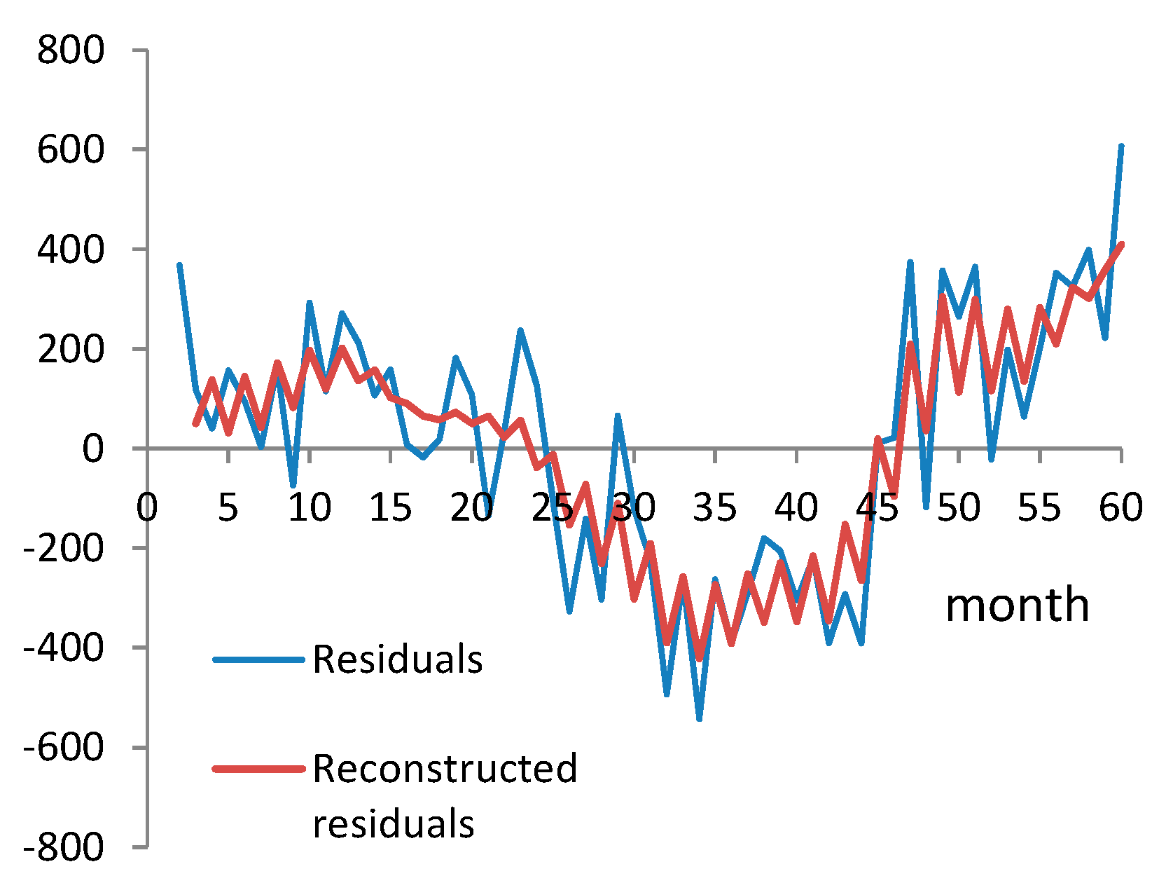
Date	Error	Date	Error	Date	Error	Date	Error	Date	Error
Jan-2013	0	Jan-2014	212.82	Jan-2015	−105.29	Jan-2016	−290.01	Jan-2017	357.39
Feb-2013	367.80	Feb-2014	106.43	Feb-2015	−327.16	Feb-2016	−179.88	Feb-2017	265.03
Mar-2013	117.99	Mar-2014	159.30	Mar-2015	−140.29	Mar-2016	−205.51	Mar-2017	365.16
Apr-2013	39.81	Apr-2014	8.10	Apr-2015	−303.38	Apr-2016	−304.85	Apr-2017	−22.18
May-2013	157.21	May-2014	−17.18	May-2015	66.35	May-2016	−220.61	May-2017	198.63
Jun-2013	94.13	Jun-2014	18.52	Jun-2015	−121.90	Jun-2016	−390.18	Jun-2017	64.66
Jul-2013	2.69	Jul-2014	182.20	Jul-2015	−225.45	Jul-2016	−291.71	Jul-2017	200.08
Aug-2013	163.54	Aug-2014	107.07	Aug-2015	−494.10	Aug-2016	−391.72	Aug-2017	352.42
Sep-2013	−74.15	Sep-2014	−133.66	Sep-2015	−260.77	Sep-2016	11.28	Sep-2017	324.36
Oct-2013	292.91	Oct−2014	33.12	Oct-2015	−542.59	Oct-2016	21.84	Oct-2017	398.30
Nov-2013	115.52	Nov−2014	236.83	Nov-2015	−263.04	Nov-2016	375.05	Nov-2017	221.93
Dec-2013	271.25	Dec−2014	125.73	Dec-2015	−389.28	Dec-2016	−118.10	Dec-2017	606.78

.

Modeling the residual error series uses window length of L = 10, T = 59, and K = 50. The residual error matrix (trajectory matrix) is as follows:

$$M={\left[{\epsilon }_{i,j}\right]}_{i,j=1}^{10\times 50}=\left[\begin{array}{ccccc}367.80& 117.99& 39.81& \cdots & 365.16\\ 117.99& 39.81& 157.21& \cdots & -22.18\\ 39.81& 157.21& 94.13& \cdots & 198.63\\ ⋮& ⋮& ⋮& \ddots & ⋮\\ 115.51& 271.25& 212.82& \cdots & 606.78\end{array}\right],$$

(58)

Eigenvalues and corresponding eigenvectors of the matrix $S=M{M}^{\mathrm{T}}\in R^{10\times 10}$ are shown in

Table 6. Decreasing order of eigenvalues and corresponding eigenvectors.

	${\mathbf{\lambda }}_{\mathbf{1}}$	${\mathbf{\lambda }}_{\mathbf{2}}$	${\mathbf{\lambda }}_{\mathbf{3}}$	${\mathbf{\lambda }}_{\mathbf{4}}$	${\mathbf{\lambda }}_{\mathbf{5}}$
Eigenvalue	16852400.60	3998636.19	2460060.01	1802229.97	1332471.93
$log$	7.227	6.602	6.391	6.256	6.125
Contribution	0.56197	0.13334	0.08203	0.06010	0.04443
Eigenvector	$U_1$	$U_2$	$U_3$	$U_4$	$U_5$
1	−0.2696	−0.4300	0.2286	0.4210	0.2918
2	−0.2767	−0.3702	−0.3707	0.2938	0.2496
3	−0.3009	−0.3767	0.2005	0.0958	−0.2846
4	−0.3086	−0.2016	−0.4298	−0.1969	−0.4163
5	−0.3197	−0.1666	0.2992	−0.4384	−0.3432
6	−0.3336	0.0749	−0.3571	−0.4185	0.2514
7	−0.3397	0.1139	0.3876	−0.3197	0.4439
8	−0.3442	0.3538	−0.2147	0.0509	0.2956
9	−0.3317	0.3311	0.3865	0.2241	−0.1589
10	−0.3280	0.4630	−0.1502	0.4075	−0.3280
	${\mathbf{\lambda }}_{\mathbf{6}}$	${\mathbf{\lambda }}_{\mathbf{7}}$	${\mathbf{\lambda }}_{\mathbf{8}}$	${\mathbf{\lambda }}_{\mathbf{9}}$	${\mathbf{\lambda }}_{\mathbf{10}}$
Eigenvalue	1169850.94	841474.95	679539.923	451182.92	400094.859
$log$	6.068	5.925	5.832	5.654	5.602
Contribution	0.03901	0.02806	0.02266	0.01505	0.01334
Eigenvector	$U_6$	$U_7$	$U_8$	$U_9$	$U_{10}$
1	0.4615	−0.0659	0.4139	0.1834	−0.0744
2	−0.2947	−0.3348	−0.3930	−0.2625	0.2796
3	−0.2062	0.6338	−0.2718	−0.1146	−0.3254
4	−0.2387	−0.1172	0.3348	0.5331	0.0157
5	0.2606	−0.1656	0.0905	−0.4260	0.4307
6	0.3713	−0.0910	−0.1588	−0.1483	−0.5691
7	−0.1663	0.0637	−0.2896	0.5020	0.2334
8	−0.2252	0.4277	0.4966	−0.3136	0.2041
9	−0.3645	−0.4860	0.1112	−0.1246	−0.3981
10	0.4286	0.0960	−0.3347	0.1753	0.2148

.

The point p, which divides residual error series into the signal and noisy subset, was selected according to the logarithm eigenvalues plot and contribution of eigenvalues (see Figure 5 and Table 6).

The value of p was selected with respect to the contribution of eigenvalues and is p = 6. Corresponding vectors $U_1,U_2,\dots ,U_6$ were included in the reconstruction phase of the residual error series. It indicates that the reconstructed trajectory matrix will be expressed as the sum of six reconstructed matrices, $\widehat{M}={{\displaystyle \sum }}_{i=1}^6{U}_i{U}_i^{\mathrm{T}}M={\widehat{M}}_1+{\widehat{M}}_2+\dots +{\widehat{M}}_6$. Applying the Hankelization on each reconstructed matrix, we obtained the following six reconstructed series of residual errors (see Figure 6).

The reconstructed residual error series was obtained by summing up these six series and the result is represented by Figure 7.

The final predicted metal price series was obtained by adding the reconstructed residuals to the predicted lead metal prices. The results of the model are represented in

Table 7. Predicted values of the metal price obtained by the SGDE+SSA model.

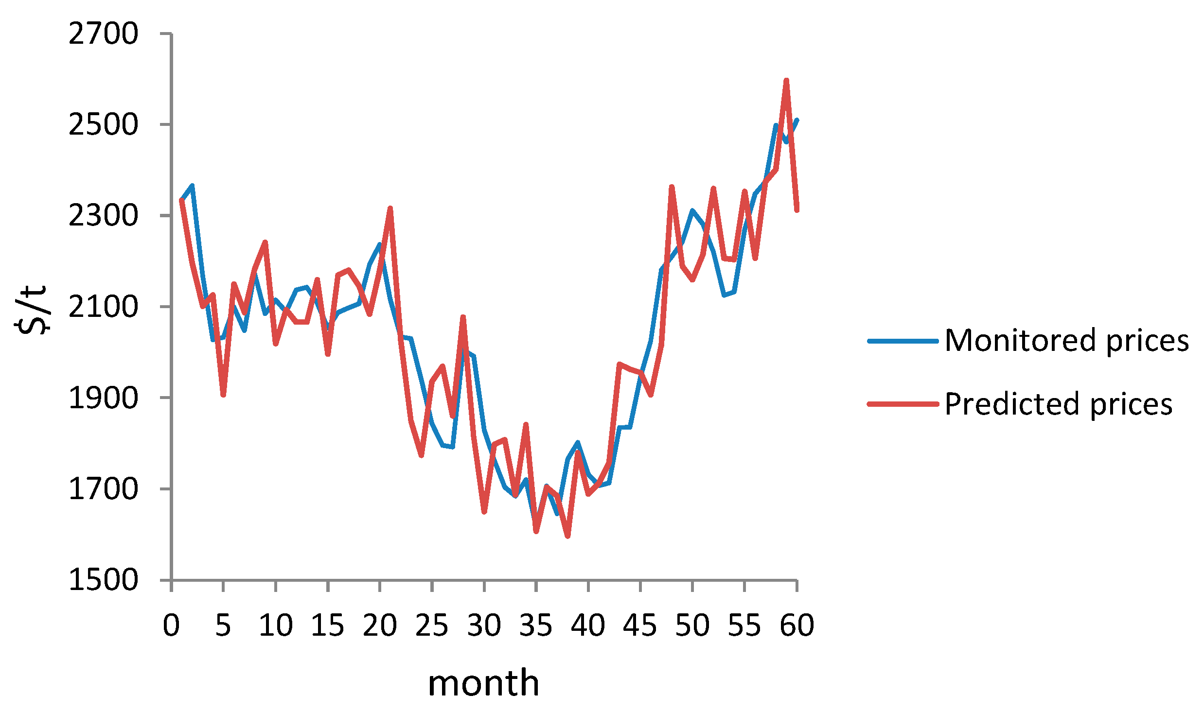
Date	Price $/t	Date	Price $/t	Date	Price $/t	Date	Price $/t	Date	Price $/t
Jan-2013	2334	Jan-2014	2066	Jan-2015	1936	Jan-2016	1684	Jan-2017	2190
Feb-2013	2197	Feb-2014	2159	Feb-2015	1969	Feb-2016	1597	Feb-2017	2159
Mar-2013	2101	Mar-2014	1996	Mar-2015	1860	Mar-2016	1779	Mar-2017	2215
Apr-2013	2126	Apr-2014	2169	Apr-2015	2077	Apr-2016	1690	Apr-2017	2359
May-2013	1907	May-2014	2180	May-2015	1815	May-2016	1712	May-2017	2206
Jun-2013	2150	Jun-2014	2146	Jun-2015	1650	Jun-2016	1757	Jun-2017	2203
Jul-2013	2088	Jul-2014	2084	Jul-2015	1798	Jul-2016	1974	Jul-2017	2353
Aug-2013	2182	Aug-2014	2179	Aug-2015	1808	Aug-2016	1963	Aug-2017	2206
Sep-2013	2242	Sep-2014	2316	Sep-2015	1688	Sep-2016	1955	Sep-2017	2374
Oct-2013	2020	Oct-2014	2024	Oct-2015	1841	Oct-2016	1907	Oct-2017	2402
Nov-2013	2094	Nov-2014	1849	Nov-2015	1607	Nov-2016	2014	Nov-2017	2598
Dec-2013	2067	Dec-2014	1774	Dec-2015	1704	Dec-2016	2363	Dec-2017	2312

Note: SGDE+SSA—Stochastic Grey Differential Equation and Singular Spectrum Analysis.

and Figure 8.

The data ranging from January 2018 to December 2019 were collected to estimate the forecasting capability of the SGDE+SSA model. Actual and forecasted metal prices and residual errors are represented in

Table 8. Forecasted metal prices.

Date	Price $/t	Forecasted Price $/t	Error	Error %	|Error| %
Jan-2018	2584	2107	−478	−18.48	18.48
Feb-2018	2581	2338	−243	−9.42	9.42
Mar-2018	2390	2235	−155	−6.49	6.49
Apr-2018	2352	2479	127	5.38	5.38
May-2018	2361	2504	143	6.04	6.04
Jun-2018	2436	2400	−36	−1.48	1.48
Jul-2018	2207	2679	472	21.40	21.40
Aug-2018	2054	2437	383	18.66	18.66
Sep-2018	2023	2490	467	23.11	23.11
Oct-2018	1988	2197	209	10.53	10.53
Nov-2018	1937	2501	563	29.09	29.09
Dec-2018	1972	2606	634	32.15	32.15
Jan-2019	1997	1989	−8	−0.41	0.41
Feb-2019	2063	2210	147	7.14	7.14
Mar-2019	2046	2032	−14	−0.68	0.68
Apr-2019	1939	2263	324	16.69	16.69
May-2019	1815	2240	425	23.42	23.42
Jun-2019	1900	2123	223	11.76	11.76
Jul-2019	1976	2373	397	20.10	20.10
Aug-2019	2045	2120	75	3.67	3.67
Sep-2019	2072	2156	84	4.07	4.07
Oct-2019	2184	1857	−327	−14.99	14.99
Nov-2019	2021	2142	121	6.00	6.00
Dec-2019	1901	2258	357	18.80	18.80

and by Figure 9.

Accuracy of the developed methods used for modeling the lead metal price series is represented in

Table 9. SGDE and SGDE+SSA model accuracy.

Model	Phase	MAPE
SGDE+SSA	Prediction (Jan-2013 to Dec-2017)	4.37%
	Forecasting (Jan-2018 to Dec-2019)	12.92%

Note: MAPE—Mean Average Percentage Error.

.

Alipour et al. [9] made a comparison between the linear prediction method ARIMA, nonlinear TGARCH, and stochastic SDE. We used their results to check the effectiveness of our model (

Table 10. The comparison between ARIMA, TGARCH, SDE, and SGDE+SSA.

Time	Price ($/t)	ARIMA (2,1,3) ($/t)	TGARCH (1,1) ($/t)	SDE ($/t)	SGDE+SSA ($/t)
Jan.2015	5830.54	6305.05	8227.29	5862.61	5830.54
Feb.2015	5729.27	6319.53	8247.58	5862.49	5651.84
March 2015	5939.67	6334.01	8267.89	5858.46	5919.15
April.2015	6042.09	6348.48	8288.19	5870.12	6197.98
May 2015	6294.78	6362.96	8308.50	5892.55	6188.28
June 2015	5833.01	6377.43	8328.80	5919.63	5738.34
July 2015	5456.75	6391.91	8349.11	5948.18	5555.65
Aug. 2015	5127.30	6406.38	8369.41	5984.84	5247.37
Sept. 2015	5217.25	6420.86	8389.72	6014.61	5159.78
Oct. 2015	5216.09	6435.34	8410.01	6039.24	5022.23
Nov. 2015	4799.90	6449.81	8430.33	6055.98	4952.51
Dec. 2015	4638.83	6464.29	8450.62	6091.78	4551.01
Jan. 2016	4471.79	6478.76	8470.93	6117.63	4595.83
Feb. 2016	4598.62	6493.24	8491.23	6110.95	4627.92
March 2016	4953.80	6507.72	8511.54	6129.23	4850.03
April.2016	4872.74	6522.19	8531.84	6170.89	4876.21
May 2016	4694.54	6536.67	8552.15	6206.12	4708.76
June 2016	4641.97	6551.14	8572.45	6218.98	4629.30
July 2016	4864.90	6565.62	8592.76	6243.33	4867.50
Aug. 2016	4751.67	6580.10	8613.05	6263.15	4637.87
Sept. 2016	4722.20	6594.57	8633.36	6291.74	4847.93
Oct. 2016	4731.26	6609.05	8653.66	6313.25	4925.22
Nov. 2016	5450.93	6623.52	8673.97	6336.70	5260.36
Dec. 2016	5660.35	6638.00	8694.27	6341.77	5592.02
Jan. 2017	5754.56	6652.48	8714.58	6362.59	5886.36
Feb. 2017	5940.91	6666.95	8734.88	6361.37	5863.69
March 2017	5824.63	6681.43	8755.19	6373.59	5742.58
April.2017	5683.90	6695.90	8775.49	6382.08	5818.67
May 2017	5599.56	6710.38	8795.80	6400.39	5463.98
June 2017	5719.76	6724.86	8816.10	6412.17	5778.85
July 2017	5699.48	6739.33	8836.40	6406.76	5976.38
Aug. 2017	5978.60	6753.81	8856.70	6395.39	5839.70
Sept. 2017	6478.35	6768.28	8877.01	6443.90	6125.46
MAPE (%)		20.90	54.36	15.61	2.04

Notes: TGARCH—Threshold Generalized Autoregressive Conditional Heteroskedasticity; ARIMA—Autoregressive Integrated Moving Average.

).

The comparative analysis of testing period performance of the ARIMA, TGARCH, SDE, and SGDE+SSA techniques, using MAPE criterion, has been accomplished and is shown in Table 10. According to the table, for the ARIMA, TGARCH, SDE, and SGDE+SSA models, the MAPE values are 20.90%, 54.36%, 15.61%, and 2.04%, respectively. The results indicate that the prediction capability of the SGDE+SSA model is higher in comparison with ARIMA, TGARCH, and SDE. It can be seen that the SDE model is superior over the linear and nonlinear models. It indicates that our approach of merging nonlinear and stochastic techniques is a well-stated hypothesis.

4. Conclusions

Strategic planning is very important in the mining industry (business) to make a profitable and sustainable production plan. The main source of uncertainty is metal price, which has a significant influence on planning. The aim of this paper was to understand and describe the behavior of metal price. The proposed approach used Stochastic Grey modelling to roughly predict the next price from a set of recent data, and then used the Singular Spectrum Analysis to fit residual error. Through simulation results, this paper offers an effective novel model to deal with the high fluctuation sequence, such as metal price series. It offers a better accuracy prediction than traditional Grey modelling. This study is important for metal mining companies, because they can forecast the metal price behavior. The developed model enables companies to reduce the metal price risks and to increase the efficiency of their operations. Comparative analysis has shown that the developed model can be applied to forecast any mineral commodity. Also, it can be applied for any time series analysis and to forecast future values of many economic commodities having high fluctuation.

Future research will be directed to the creation of stochastic-grey differential equation, which will be capable of incorporating jumps into metal price forecasts. The length of observed time series data plays a key role in modelling. A small sample of data can increase the accuracy of the prediction, but it is nonsufficient for capturing the real behavior. Also, this issue can be the subject of further research.

References

- Barczak, S. Gold Price Forecasting Using Grey Model GM(1,1) and Selected Classical Time Series Models. A Comparison of Methods. In Proceedings of the 8th International Days of Statistics and Economics, Prague, Czech Republic, 11–13 September 2014. [Google Scholar]
- Askari, M.; Askari, H. Time Series Grey System Prediction-based Models: Gold Price Forecasting. Trends Appl. Sci. Res. 2011, 6, 1287–1292. [Google Scholar] [CrossRef]
- Chang, C.J.; Li, D.C.; Chen, C.C.; Dai, W.L. A grey-based rolling procedure for short-term forecasting using limited time series data. Econ. Comput. Econ. Cybern. Stud. Res. 2013, 47, 75–90. [Google Scholar]
- Jalali, M.F.M.; Heidari, H. Forecasting Palladium Price Using GM(1,1). Glob. Anal. Discret. Math. 2018, 3, 1–9. [Google Scholar] [CrossRef]
- Sous, S.; Thongjunthug, T.; Klongdee, W. Gold price forecasting based on the improved GM(1,1) model with Markov chain by average of middle points. KKU Sci. J. 2014, 42, 693–699. [Google Scholar]
- Yang, S.; Chen, J.H.; Guo, H.B.; Liao, G.S. Application of optimal unbiased grey-forecasting model in aluminum price quotation prediction. J. Hunan Univ. Sci. Technol. (Nat. Sci. Ed.) 2012, 2. [Google Scholar]
- Wang, K.G.; Zheng, Z.Q.; Yang, X.M. The Comparative Research of Mine Price Forecast Based on the Gray System GM(1,1) Model and the Model of Verhulst. J. Gansu Sci. 2014, 5. [Google Scholar]
- Li, D.; Moghaddam, M.R.; Monjezi, M.; Armaghani, D.J.; Mehrdanesh, A. Development of a Group Method of Data Handling Technique to Forecast Iron Ore Price. Appl. Sci. 2020, 10, 2364. [Google Scholar] [CrossRef] [Green Version]
- Alipour, A.; Khodaiari, A.A.; Jafari, A. Modeling and Prediction of Time-Series of Monthly Copper Prices. Int. J. Min. Geo-Eng. 2019, 53, 91–97. [Google Scholar] [CrossRef]
- Shafiee, S.; Topal, E. Introducing a new model to forecast mineral commodity price. In Proceedings of the First International Future Mining Conference and Exhibition, Sydney, Australia, 19–21 November 2008; pp. 243–250. [Google Scholar]
- Achireko, P.K.; Ansong, G. Stochastic model of mineral prices incorporating neural network and regression analysis. Min. Technol. 2000, 109, 49–54. [Google Scholar] [CrossRef]
- Tapia Cortez, C.A.; Saydam, S.; Coulton, J.; Sammut, C. Alternative techniques for forecasting mineral commodity prices. Int. J. Min. Sci. Technol. 2018, 28, 309–322. [Google Scholar] [CrossRef]
- Deng, J. Grey control system. J. Huazhong Univ. Sci. Technol. 1982, 10, 9–18. [Google Scholar]
- Deng, J.L. Control problems of grey systems. Syst. Control. Lett. 1982, 1, 288–294. [Google Scholar]
- Liu, S.F.; Zeng, B.; Liu, J.; Xie, N.M. Several basic models of GM(1,1) and their applicable bound. Syst. Eng. Electron. 2014, 36, 501–508. [Google Scholar]
- Dang, Y.; Liu, S.; Chen, K. The GM models that x(n) be taken as initial value. Kybernetes 2004, 33, 247–254. [Google Scholar]
- Evans, L.C. An Introduction to Stochastic Differential Equations—Version 1.2. Available online: http://ft-sipil.unila.ac.id/dbooks/AN%20INTRODUCTION%20TO%20STOCHASTIC%20DIFFERENTIAL%20EQUATIONS%20VERSION%201.2.pdf (accessed on 7 August 2020).
- Reis, M. Stochastic Differential Equation. Lecture Notes at Humboldt University Berlin and University of Heidelberg. 2007. Available online: https://www.math.uni-heidelberg.de/studinfo/reiss/sode-lecture.pdf (accessed on 7 August 2020).
- Bayram, M.; Partal, T.; Buyukoz, G.O. Numerical methods for simulation of stochastic differential equations. Adv. Differ. Equ. 2018, 17, 1–10. [Google Scholar] [CrossRef] [Green Version]
- Sauer, T. Numerical solution of stochastic differential equation in finance. In Handbook of Computational Finance; Springer: Berlin, Germany, 2012; pp. 529–550. [Google Scholar]
- Schwarz, E.S. The stochastic behavior of commodity prices: Implications for valuation and hedging. J. Financ. 1997, 52, 923–973. [Google Scholar] [CrossRef]
- Chapter 4, Brownian Motion and Stochastic Calculus, This Version. 15 January 2020. Available online: https://www.ntu.edu.sg/home/nprivault/indext.html (accessed on 9 February 2020).
- Hassani, H.; Mahmoudvand, R. Multivariate Singular Spectrum Analysis: A general view and new vector forecasting approach. Int. J. Energy Stat. 2013, 1, 55–83. [Google Scholar] [CrossRef]
- Hassani, H.; Zhigljavsky, A. Singular Spectrum Analysis: Methodology and Application to Economics Data. J. Syst. Sci. Complex. 2009, 22, 372–394. [Google Scholar] [CrossRef]
- Hassani, H. Singular Spectrum Analysis: Methodology and Comparison. J. Data Sci. 2007, 5, 239–257. [Google Scholar]
- Harris, T.J.; Yuan, H. Filtering and frequency interpretations of Singular Spectrum Analysis. Phys. D 2010, 239, 1958–1967. [Google Scholar] [CrossRef]
- Steel Success Strategies. 2020. Available online: https://www.indexmundi.com/commodities/?commodity=lead&months=120 (accessed on 14 April 2020).