Reductions in CO₂ Emissions from Passenger Cars under Demography and Technology Scenarios in Japan by 2050

Abstract

Climate policy requires substantial reductions in long-term greenhouse gas (GHG) emissions, including in the transportation sector. As passenger cars are one of the dominant CO₂ emitters in the transport sector, governments and the automobile industry have implemented various countermeasures, including decarbonization of fuels, more energy efficient vehicles, and transport demand management. However, the total impact of these measures in the long term remains unclear. This study aims to clarify the CO₂ emissions reductions from passenger cars by 2050 in 1727 municipalities in Japan under a declining population. To estimate CO₂ emissions, we model travel behavior and traffic situations reflecting the regional conditions of the municipalities, including population density and accessibility to public transport for the base year 2010. Assuming plausible scenarios for future populations and automobile technologies, we estimate CO₂ emissions from passenger cars. We estimate that CO₂ emissions will decline by 64–70% between 2010 and 2050, with automobile technologies playing the largest role. We find that the impact of urban compaction is marginal at the national level but varies by municipality. These results imply that, given regional variations, all countermeasures, including technology and demand management, must be used to achieve the long-term target of CO₂ emissions reductions.

1. Introduction

The transport sector accounted for 23% of global CO₂ emissions in 2010, and its share of emissions is expected to increase at a higher rate than that of other sectors towards 2050 [1]. Road transport is a dominant source of emissions, accounting for 70% of transport sector emissions. Furthermore, 80% of road transport emissions come from passenger transport [2]. Consequently, substantial reductions in CO₂ emissions from passenger cars are required, and various countermeasures are expected to reduce these emissions. The countermeasures include reducing carbon intensity [3,4], improving the energy efficiency of vehicles [5,6,7,8], electrification of vehicles [9,10], and reducing vehicle weights [11], as well as demand management measures, such as traffic control and modal shift policies [12,13,14,15] and urban compaction [16,17,18,19,20,21].

The technological measures are expected to be effective everywhere if the technologies are diffused effectively in the market, whereas the impact of demand management measures varies depending on the regional conditions. The International Energy Agency (IEA) estimated that technological measures would reduce greenhouse gas (GHG) emissions in the transport sector by 54% from 2015 to 2060 under the “2 degree scenario” and by 83% for the same period in the “beyond 2 degree scenario” [22], in which a very ambitious technology deployment rate is assumed. In regard to demand management, Cuenot et al. [23] estimated the effect of a modal shift that reduced automobile and air traffic by 25% globally by 2050. Their analysis was based on national level statistics and did not consider subnational conditions. Using Japanese statistics for 1980–2005, Matsuhashi and Ariga [24] clarified that an area with a higher population density emits less CO₂ from automobiles. On the basis of this statistical relationship, they estimated CO₂ emissions from automobiles for whole municipalities in Japan in 2030. They estimated that urban compaction would reduce CO₂ emissions by 5% compared with a sprawled urban pattern. However, they did not consider the improvement of automobile technologies.

Studies analyzing mitigation impacts on a global scale usually simplify the transport demand conditions, and most do not consider spatial policies such as urban compaction. Meanwhile, the studies analyzing the impact of spatial policies usually do not consider vehicle technologies. To estimate the future potential to reduce CO₂ emissions, we need to incorporate both technology and demand management. In this study, we estimate the CO₂ emissions from passenger cars in 1727 municipalities in Japan by 2050 and analyze the factors affecting the emissions, considering both automobile technologies and travel demand. On the basis of this analysis, we clarify the impact of the scenarios on automobile CO₂ emissions quantitatively and discuss the possible measures for substantial emissions reductions. The impact of the factors influencing emissions under depopulation, demographic change, and spatial shift of activities is not clarified sufficiently in the existing literature. Our research advances the CO₂ mitigation studies in the transport sector by considering automobile technologies, demography, and spatial feature of regions simultaneously.

2. Analytical Framework and Method

Our analytical framework to estimate CO₂ emissions is based on breaking down emissions into activity (A), modal structure (S), modal energy intensity (I), and carbon content of fuels (F), known as the ASIF approach [25,26]. This approach analyzes the emissions reduction potential of each factor and the interaction among the factors. In this study, we consider the energy sources as gasoline, diesel, electricity, and hydrogen. The well-to-wheel carbon contents of these sources are given by scenarios based on the literature. The energy efficiencies of vehicles by energy sources are also given by the scenarios. In the real world, emissions are affected by road speed. We quantify the regional road speed distribution based on traffic volumes and road supply. Traffic volumes are quantified based on demography and urban policies. To estimate the travel demand, we formulate the go out rate and the net trip rate by gender and age classes. Furthermore, we estimate the average occupancy rate of a vehicle and the average car trip length. The explanatory variables of these models are the urban conditions, including population and transportation facilities. We assume that there are three transport modes: cars, public transport, and walking/cycling. The modal shares of each are formulated using the explanatory variables for the urban conditions. The analytical framework is depicted in Figure 1.

We denote CO₂ emissions from passenger cars in municipality i in year t as $CO{2}_{ti}$, which is formulated as follows:

$$CO{2}_{ti} = {\epsilon }_t\left(x_{ti}\right)\frac{L\left(x_{ti}\right)}{\rho \left(x_{ti}\right)}{\displaystyle \sum }_k{N}_{ck}\left(x_{ti}\right)$$

(1)

where $x_{ti}$ is the attribute vector of the municipality, ${\epsilon }_t$ is the average real-world emissions factor of in-use vehicles, $L$ is the trip length of passenger cars, $\rho$ is the occupancy ratio, and $N_{ck}$ is the number of trips of a user of attribute k.

$N_{ck}\left(x_{ti}\right)$ is expressed in the form:

$$N_{ck}\left(x_{ti}\right) = tp{p}_i·S_{tki}·go{r}_{tki}\left(x_{ti}\right)·nt{g}_{tki}\left(x_{ti}\right)·P{r}_{ctki}\left(x_{ti}\right)$$

(2)

where $tp{p}_i$ is the total population, $S_{tki}$ is the population share of people with attribute k, $go{r}_{tki}$ is the go-out rate, $nt{g}_{tki}$ is net trips per person, and $P{r}_{ctki}$ is the modal share of passenger cars.

These functions and emission factors are determined in Section 4 using the data explained in the next section. As formulated in Equation (2), we use individual projection for the car travel demand. Some studies projected car travel demand using household projection because the purchase and the usage of cars are usually decisions by households, not individuals. The probable effect of using the individual projection instead of household projection is addressed in Section 6.

3. Data and Scenarios

In this study, we use the “nationwide person trip survey” [27] for travel pattern data and “mesh statistics and projections” [28] for data on the urban population, its density, and the urban area. Public transport facilities are given by the geographic information database of the Ministry of Land, Infrastructure, and Transport (MLIT) of Japan [28]. Road traffic and speed data are provided by the National Road Census [29]. In the following subsections, we provide a summary of these data and describe future scenarios of urban features and automobile technologies.

3.1. Data

3.1.1. Nationwide Person Trip Survey

The nationwide person trip survey is conducted every 5 years and compiles travel behavior data, including trip purpose, travel modes, and number of trips, for selected cities in Japan. We use the data for 2010. A total of 130 cities were surveyed in 2010, including 70 large cities, in each of which 500 households are sampled. The data include age, gender, and travel behavior of the household members. The remaining 60 cities are small cities, in which 50 households were surveyed to collect the same data as for the large cities.

3.1.2. Population Projections and Spatial Distribution

We use the mesh population data [28] for the municipality population projections and spatial distributions. This data source provides the population by attribute for each 500 m × 500 m mesh, covering the entire land area of Japan. The base year of these data is 2010, and the mesh population in the base year is given by the national census. The future mesh populations are projected consistent with the population projections for all municipalities by the National Institute of Population and Social Security Research (IPSS) [30]. The mesh data include population projections by gender and age classes for all 5-year periods up to 2050. For reference, the population trajectory by age class from 1965 to 2065 compiled by the IPSS is shown in Figure 2.

On the basis of these spatial population data, we define the urban area as meshes with a population density of over 40 people/ha and calculate the urbanized area of the municipality. The urban population is the sum of the populations in the urban meshes, and the urban population ratio is the ratio of the urban population to the total population in the municipality. We define the “urban geometric moment” as the sum of the products of the mesh populations and the mesh distance from the population centroid of a municipality divided by the total population of the municipality. It is used as a representative index of the urban spatial scale.

3.1.3. Public Transport Catchment Area

The location coordinates of railway stations and bus stops are obtained from the national land information system [28]. We assume that the catchment area of a bus stop (railway station) is a circular area within a 300 m (800 m) radius from the bus stop (station) based on the definitions provided by the MLIT. We calculate the catchment population as the sum of the population of the meshes that intersect with the catchment area. The merged catchment area of a bus stop and railway station is defined as the public transport catchment area. Figure 3 shows the catchment area in the case of the town of Chippubetsu, Hokkaido. The black polygon shows the administrative area of the town, the gray edged meshes indicate the out-of-catchment area, the small red circles show the bus stop catchment areas, the large red circles shows the rail station catchment areas, and the blue edged meshes intersecting with the catchment circles are defined as the meshes of the public transport catchment areas.

3.1.4. Road Traffic Census

The National Road Census [29] provides publicly available road statistics. The data for 2015 include traffic volume, peak traffic ratio, speeds for congested and noncongested travel time, road link length, and number of lanes for approximately 97,000 road links. Owing to data limitations, it is difficult to estimate the impact of traffic on road speed for each link. As there are many observed links in this data set, we expect to capture the regional features of road speed and traffic by using the regionally pooled data.

3.2. Future Scenarios

The major drivers affecting CO₂ emissions include population change, urban structure change, and the progress of automobile technologies. In this study, the urban structure is defined by the spatial distribution of the population and, therefore, population change induces urban structure change. The baseline scenario of the spatial distribution of the population is given by the MLIT. We generate a compact scenario for the future urban structure. In this compact scenario, the total population for each municipality is the same as in the baseline scenario, but we assume that the populations decline in the meshes of the municipalities that have the smallest populations. In other words, the compact scenario assumes that the population becomes zero for the meshes with the smallest populations to meet the given municipality population decline. This is an extreme case of urban compaction. Figure 4 shows the spatial distribution of the population in 2010 and baseline and compact scenarios in 2050. In the case of the baseline scenario, the meshes of the low population density areas are distributed over a wide area. By contrast, in the compact scenario, we observe that the population meshes are located within a very limited area.

In this study, we consider five automobile technologies that have different CO₂ emissions factors: (1) gasoline, (2) diesel, (3) hybrid electric vehicles (HEV), (4) electric vehicles/plug-in hybrid electric vehicles (EV/PHEV), and (5) fuel cell vehicles (FCV). The share of vehicles in-use by these technologies until 2030 are determined based on the “roadmap for EV/PHEV” [31] and the “new strategic roadmap for hydrogen and fuel cells” [32]. We calculate the sales share of the vehicles by technologies to ensure consistency with the in-use share, assuming a survival curve for automobiles under which their maximum duration is 20 years. After 2030, the sales share by technologies is determined based on the 2 °C Scenario (2DS) improve scenario in IEA Energy Technology Perspectives (ETP) 2012 [33]. Applying the survival curve to the sales scenario, we estimate the share of in-use automobiles by technologies. Figure 5 shows the sales share and the in-use vehicle shares for the five technologies.

“The Plan for Global Warming Countermeasures” [34] sets a target for average fuel economy by 2030. We determine the improvement in fuel economy for new gasoline and diesel vehicles by referring to this plan. We assume that the fuel economies of gasoline and diesel technologies reach their upper limit in 2030 and do not change after this. On the basis of this assumption, we calculate the average fuel economy of the in-use vehicles. We fix the energy efficiency of the other technologies at the 2010 level, but the emissions from electric power generation are assumed to improve, reflecting the voluntary target of 370 g CO₂/kWh by 2030 set by the Federation of Electric Power Companies of Japan [35]. After 2030, we have no information on the emissions reduction target for electric power generation, thus we simply fix the emissions factor in our scenario. For real-world fuel efficiency, we assume that HEV and EV/PHEV consume 67% more energy than is the case for test cycle fuel efficiency and that the other technologies, gasoline, diesel, and FCV, consume 43% more. The assumed CO₂ emission factors by automobile technologies and average emission factors of in-use vehicles are summarized in

Table 1. CO₂ emissions factors by automobile technologies and in-use average (g CO₂/km).

	Gasoline	Diesel	HEV	EV/PHEV	FCV	Average
2010	228	244	128	84	123	226
2020	197	197	128	97	123	182
2030	169	170	128	75	123	143
2040	166	164	128	75	123	129
2050	166	164	128	75	123	114

HEV: hybrid electric vehicles; EV/PHEV: electric vehicles/plug-in hybrid electric vehicles; FCV: fuel cell vehicles.

.

4. Model

In this section, we explain the models that we construct to estimate traffic volume and CO₂ emissions, using the data for 130 municipalities described in Section 3. For each municipality, we estimate: (1) trip generation, (2) modal split, (3) vehicle occupancy ratio, and (4) trip length by car. Multiplying the estimated vehicle-kms and CO₂ emissions factors, we estimate the total volume of CO₂ emissions. Using this model, we estimate the future emissions for every 5 years from 2020 to 2050 and decompose the emissions by factors of technologies, road speed, population, demography, and urban structure under the scenarios explained above.

4.1. Model Estimation

First, we model the go-out rate and the net trip generation by gender and age classes using linear regression analysis. Second, the modal split is represented by a nested logit model. The lower level model is the choice between car and public transport, which is in the motorized transport nest. The upper level model is the choice between motorized and nonmotorized (walking/cycling) transport. The third and the fourth models are linear regression models used to model vehicle occupancy ratio and car trip length, respectively. All the above regression models are estimated using stepwise regression and the backward elimination approach to maximize the Akaike information criterion.

4.1.1. Go-Out Rate Model

By stepwise regression, we obtain the following formula to estimate the go-out rate $go{r}_{tki}$ of people with attribute k in municipality i in year t:

$$go{r}_{tki} = {\alpha }_{gk0}+{\alpha }_{gk1}·tp{p}_{ti}+{\alpha }_{gk2}·urb{A}_{ti}+{\alpha }_{gk3}·pop{D}_{ti}$$

(3)

where $tp{p}_{ti}$ is the total population, $urb{A}_{ti}$ is the area of the urban area, $pop{D}_{ti}$ is population density, and ${\alpha }_{gk0}$, ${\alpha }_{gk1}$, ${\alpha }_{gk2}$, and ${\alpha }_{gk3}$ are parameters.

The estimated parameters are shown in

Table 2. Estimated parameters of the go-out rate model.

Gender	Male				Female
Age	−14	15–64	65–74	75–	−14	15–64	65–74	75–
Intercept	1.01	0.92	0.82	0.73	0.99	0.85	0.69	0.40
	(174.1)	(543.1)	(80.7)	(27.1)	(392.2)	(132.1)	(41.0)	(20.9)
tpp	1.01 × 10−8	2.72 × 10−9	NA	2.35 × 10−8	8.66 × 10−9	8.04 × 10−9	2.79 × 10−8	−4.58 × 10−8
	(4.157)	(7.077)		(5.089)	(3.889)	(2.979)	(3.941)	(−5.752)
urbA	−1.02 × 10−4	NA	NA	NA	−1.27 × 10−4	−1.52 × 10−4	−4.26 × 10−4	7.71 × 10−4
	(−2.590)				(−3.315)	(−3.466)	(−3.703)	(5.954)
popD	−2.88 × 10−6	NA	1.49 × 10−6	−1.29 × 10−5	NA	3.94 × 10−6	1.06 × 10−5	1.37 × 10−5
	(−3.789)		(1.628)	(−3.525)		(4.667)	(4.777)	(5.506)
R2	0.179	0.284	0.021	0.197	0.150	0.432	0.597	0.557

( ) t-value.

. NA indicates rejected variables.

The intercept is the go-out rate when all other variables are zero. This parameter is lower for elderly people and females. The parameters of the total population are significantly positive except for males aged 65–74 years and females over 75 years. This means that most classes of people tend to go out from their homes in larger cities.

4.1.2. Net Trip Generation Model

Net trip generation refers to the average number of trips of a person who goes out from home. The net trip number $nt{g}_{tki}$ is described as follows:

$$nt{g}_{tki} = {\alpha }_{nk0}+{\alpha }_{nk1}·tp{p}_{ti}+{\alpha }_{nk2}·urb{A}_{ti}+{\alpha }_{nk3}·pop{D}_{ti}$$

(4)

where ${\alpha }_{nk0}$, ${\alpha }_{nk1}$, ${\alpha }_{nk2}$, and ${\alpha }_{nk3}$ are parameters. The estimated parameters are shown in

Table 3. Estimated parameters of the net trip generation model.

Gender	Male				Female
Age	−14	15–64	65–74	75–	−14	15–64	65–74	75–
Intercept	2.59	3.07	3.37	3.06	2.70	3.17	2.93	2.89
	(36.9)	(66.8)	(135.8)	(77.8)	(121.3)	(88.1)	(67.4)	(36.5)
tpp	−8.32 × 10−8	2.64 × 10−8	NA	8.64 × 10−8	6.07 × 10−8	4.62 × 10−8	NA	7.41 × 10−8
	(−2.842)	(3.342)		(2.495)	(12.018)	(3.070)		(5.459)
urbA	1.63 × 10−3	NA	−5.27 × 10−4	−1.83 × 10−3	NA	−3.89 × 10−4	NA	NA
	(3.434)		(−6.065)	(−3.060)		(−1.589)
popD	1.65 × 10−5	−1.46 × 10−5	NA	NA	NA	−1.22 × 10−5	2.35 × 10−5	−3.87 × 10−5
	(1.799)	(−2.329)				(−2.585)	(5.983)	(−3.594)
R2	0.263	0.095	0.226	0.117	0.534	0.162	0.221	0.235

( ) t-value.

. The intercept indicates the net trip number when all explanatory variables are zero. The intercept is highest for males aged 65–74 years. There are no clear patterns in the explanatory variables based on the attributes of people. For instance, the number of trips is larger when the municipality population is larger for groups of males aged 15–64 years, males over 75 years, females less than 65 years, and females over 75 years. However, the variable does not affect males and females aged 65–74 years, and it reduces the net trips of males less than 15 years.

4.1.3. Modal Split Model

We estimate the aggregated modal share using the following nested logit model:

$$P{r}_{ctki} = \left(1-\frac{exp\left(V_{wtki}\right)}{1+exp\left(V_{wtki}\right)}\right)·\frac{exp\left(V_{ctki}\right)}{1+exp\left(V_{ctki}\right)}$$

(5)

$$V_{ctki} = {\theta }_{ck0}+{\theta }_{ck1}·pB{s}_{ti}+{\theta }_{wk2}·pR{s}_{ti}+{\theta }_{wk3}·urb{A}_{ti}+{\theta }_{wk4}·pop{D}_{ti}+{\theta }_{wk5}·up{s}_{ti},$$

(6)

$$V_{wtki} = {\theta }_{wk0}+{\theta }_{wk1}·I{V}_{kti}+{\theta }_{wk2}·pB{s}_{ti}+{\theta }_{wk3}·pop{D}_{ti}+{\theta }_{wk4}·up{s}_{ti}$$

(7)

where $P{r}_{ctki}$ is the modal share of cars, $V_{ctki}$ $and$ $V_{wtki}$ are the utilities of driving a car and of walking/cycling, respectively, $pB{s}_{ti}$ and $pR{s}_{ti}$ are the populations of the bus stop and the railway station catchment areas, respectively, and $up{s}_{ti}$ is the urban population share. $I{V}_{kti}$ is an inclusive value of the lower level model expressed as $I{V}_{kti} = \log \left(1+exp\left(V_{ctki}\right)\right)$.

Table 4. Parameters of the lower level of the modal share model.

Gender	Male				Female
Age	−14	15–64	65–74	75–	−14	15–64	65–74	75–
Intercept	3.281	3.133	4.227	4.203	0.431	3.214	2.769	4.346
	(4.339)	(5.612)	(4.757)	(4.854)	(0.401)	(5.566)	(5.617)	(2.134)
pBs	NA	NA	NA	NA	2.744	NA	NA	−3.083
					(1.791)			(−1.344)
pRs	−1.877	NA	NA	NA	NA	NA	NA	NA
	(−1.143)
urbA	4.12 × 10−3	NA	NA	NA	NA	NA	NA	−4.16 × 10−3
	(0.947)							(−1.547)
popD	−1.29 × 10−4	NA	NA	NA	−2.17 × 10−4	NA	NA	NA
	(−1.128)				(−2.616)
ups	NA	−3.029	−3.340	−3.641	NA	−3.040	−2.292	NA
		(−3.785)	(−2.833)	(−3.187)		(−3.699)	(−3.101)
R2	0.500	0.833	0.798	0.775	0.458	0.845	0.713	0.479

( ) t-value.

shows the estimated parameters of the lower level model, the choice set of which is cars and public transport. The intercept indicates the car dummy, and it is positive for all categories of people. This means that people tend to choose cars more than public transport. Among the explanatory variables, the urban population share is selected for attributes of males over 15 years and females between 15 and 74 years. This parameter is negative for these people. This means that the public transport share tends to be larger when the urban population share of the municipality is larger. For males and females aged 14 years or less, the population density parameter has a negative value. This means that public transport tends to be chosen more by these young people as population density becomes higher. These young people do not drive themselves but would be passengers accompanied by other people.

Table 5. Parameters of the upper level of the modal share model.

Gender	Male				Female
Age	−14	15–64	65–74	75–	−14	15–64	65–74	75–
Intercept	0.114	−0.564	−1.691	−1.172	0.120	−1.821	−2.115	−0.643
	(0.388)	(−1.042)	(−4.638)	(−3.978)	(0.412)	(−5.198)	(−2.003)	(−3.389)
IV	NA	−0.423	NA	NA	NA	NA	NA	NA
		(−1.717)
pBs	9.52 × 10−5	NA	9.93 × 10−5	NA	7.60 × 10−5	NA	NA	NA
	(1.820)		(1.773)		(1.493)
popD	NA	NA	NA	0.824	NA	1.564	NA	NA
				(1.547)		(2.669)
R2	0.500	0.833	0.798	0.775	0.458	0.845	0.713	0.479

( ) t-value.

shows the estimated parameters of the upper level model. The dummy parameter of walking/cycling is negative except for people aged 14 years and under. In other words, people over 15 years tend to choose motorized transport, and people under 14 tend to choose walking/cycling. The effects of the other explanatory variables differ by people’s attributes. The inclusive value (IV) is only selected for males aged 15–64 years. The sign of the parameter is negative, which means that as the utility of the motorized mode becomes higher, the probability of choosing walking/cycling becomes lower. The signs of the other explanatory variables are positive, which means that as the population within the bus catchment area becomes higher and the population density increases, the share of those choosing walking/cycling becomes higher. Except for the intercept parameter, all variables are rejected for females aged over 75 years, indicating that none of the explanatory variables affect the choice of walking/cycling for this group of people.

4.1.4. Vehicle Occupancy Rate Model

The vehicle occupancy rate ${\rho }_{ti}$ is estimated using the following form:

$${\rho }_{ti} = {\alpha }_{\rho 0}+{\alpha }_{\rho 1}·tp{p}_{ti}+{\alpha }_{\rho 2}·ug{m}_{ti}+{\alpha }_{\rho 3}·up{s}_{ti}$$

(8)

where $ug{m}_{ti}$ is an urban geometric moment, as defined above. The estimated parameters, shown in

Table 6. Parameters of the vehicle occupancy rate model.

	Parameter	(t-Value)
Intercept	1.316	(85.774)
tpp	1.66 × 10−8	(2.154)
ugm	−6.53 × 10−6	(−1.747)
ups	0.062	(3.298)
R2	0.184

, indicate that the occupancy rate becomes higher as the total population becomes larger, the urban geographic moment becomes smaller, and the urban population share becomes higher.

4.1.5. Average Car Trip Length Model

Average car trip length is estimated using the following form:

$$L_{ti} = {\alpha }_{L0}+{\alpha }_{L1}·up{s}_{ti}+{\alpha }_{L2}·ta{p}_{ti}$$

(9)

where $ta{p}_{ti}$ is the population in the public transport catchment area, which is described as $ta{p}_{ti} = tp{p}_{ti}\times S_{tr,ti}$, and $S_{tr,ti}$ is the population share of the public transport catchment area. The estimated parameters of the model are shown in

Table 7. Parameters of the car trip length model.

	Parameter	(t-Value)
Intercept	11.79	(50.02)
ups	−3.07	(−5.32)
tap	7.50 × 10−7	(3.51)
R2	0.189

. From the table, the base car trip length is about 11.8 km. The trip length is shorter when the urban population share is higher and the population of the public transport catchment area is larger. Intuitively, the population of the public transport catchment area seems to have no relation with car trip length, but this index may be used as a proxy variable of urban size.

4.1.6. Effect of Road Speed on Emissions Coefficients

The MLIT reported that the CO₂ emissions per vehicle-km ε are a function of the average travel speed v in the form:

$$\epsilon = b_0+\frac{b_1}{v}+b_2\times v+b_3\times v^2$$

(10)

where the unit of ε is gCO₂/km and v is km/h. The parameters for gasoline and diesel passenger cars in 2000 are given in

Table 8. Vehicle emissions estimation model parameters.

	b0	b1	b2	b3
Gasoline	156.05	2019	−2.087	0.01865
Diesel	285.35	1906	4.353	0.03489

[36].

Figure 6 shows the emissions curve over the road speed for gasoline vehicles using Equation (10). The emissions factor takes a minimum value around 60–70 km/h and higher values at lower speed ranges. This nonlinearity of the emissions factor requires consideration of road congestion in the emissions estimation. If we use average speed only, then we would underestimate the CO₂ emissions.

Equation (10) is relevant to the vehicles sampled in 2000. Of course, this curve differs by vehicle. As shown later, the effect of a road speed shift on the emissions factor is standardized by using the change rate of the emissions factor according to the road speed shift. Therefore, the effect has no dimension, and the level of vehicle emissions in Equation (10) does not affect future emissions.

If the road census has sufficient sample links in a municipality, then the speed distribution of the municipality can be obtained. Figure 7 shows the road speed distribution of Tokyo, Nagoya, and Osaka compiled using speed and traffic data from the national road traffic census. The horizontal axis indicates the road speed, and the vertical axis indicates the total traffic volume of the speed range. In these three cities, the peak of the distribution is around 20 km/h. The red dashed line is the log-normal probability density function fitted to the data using the maximum likelihood method. These figures indicate that the log-normal distribution can represent the road speed distribution. Hereafter, therefore, we apply the log-normal distribution to represent the speed distribution for all municipalities.

We estimate the parameters of the log-normal distribution for each municipality to fit with its speed distribution using the maximum likelihood method. If traffic volume and road supply affect the speed distribution, then we can observe the effect of them on the estimated parameters. Figure 8 shows the plot of two parameters of the log-normal distribution over the average lane traffic of municipalities.

In this figure, each point indicates the lane traffic and the estimated parameter of a municipality, and the green line is the regression line. μ is the mean parameter and it tends to decrease as lane traffic increases. σ is the standard deviation parameter, which tends to increase as lane traffic increases. This means that as the average lane traffic becomes larger, the speed distribution of a municipality becomes slower and deviates more. The estimated parameters of the regression line are shown in

Table 9. Regression parameters for the estimation of the road speed distribution.

	μ		σ
	Intercept	Traffic	Intercept	Traffic
Parameter	3.913	−6.10 × 10−5	0.149	2.37 × 10−5
t-value	126.051	−7.991	58.830	38.090
R2	0.398		0.299

.

Using the relationship among traffic, road speed, and the emissions factor, we can estimate the impact of traffic volume on the average CO₂ emissions factor ε. As the emissions factor reflects the progress of automobile technology, we need to distinguish these effects.

First, we consider the case where automobile technology is fixed. We denote p(V) as a probability density function of traffic speed V and f(V) as the emissions factor at speed V. Then, the average emission factor is expressed as follows:

$${\epsilon }_r = {{\displaystyle \int }}_0^{\infty }p\left(V\right)f\left(V\right)dV$$

(11)

Traffic change affects the speed distribution p(V), which is characterized by μ and σ. Of course, the speed distribution is affected not only by the traffic volume but also by the other factors, including density of intersections, land use, and landscape. Therefore, the relation between traffic volume and the speed distribution parameters deviates, as shown in Figure 8. In this study, we assume that the factors other than the traffic volume are fixed for each municipality and that the sensitivities of the traffic volume to these parameters are the same for all municipalities. Then, the speed distribution parameters can be calculated by the following equations using the average lane traffic q_i for municipality i:

$${\mu }_i = {\mu }_{0i}+{\alpha }_{\mu }\left(q_i-q_{0i}\right)$$

(12)

$${\sigma }_i = {\sigma }_{0i}+{\alpha }_{\sigma }\left(q_i-q_{0i}\right)$$

(13)

Here, the suffix 0 indicates the base year, 2010, and ${\alpha }_{\mu }$ and ${\alpha }_{\sigma }$ are the slopes of the regression lines in Figure 8. Denoting the emissions factor by Equation (11) at time t as ${\epsilon }_{ri}^t$ and the estimated emissions factor with fixed technology at time t + 1 as ${\epsilon }_{ri}^{t+1}$, the change rate of the emissions factor by the traffic speed change ${\alpha }_{ri}^{t+1}$ is given as:

$${\alpha }_{ri}^{t+1} = \frac{\left({\epsilon }_{ri}^{t+1}-{\epsilon }_{ri}^t\right)}{{\epsilon }_{ri}^t}$$

(14)

We denote the change rate of the emissions factor by automobile technology from t to t + 1 as ${\alpha }_T^{t+1}$. Then, the emissions factor at time t + 1, considering both traffic volume and technology, can be expressed as follows:

$${\epsilon }_i^{t+1} = \left(1+{\alpha }_T^{t+1}\right)\left(1+{\alpha }_{ri}^{t+1}\right){\epsilon }_i^t$$

(15)

Here, we assume that technological progress is disseminated to all municipalities at once. Substituting Equation (15) into Equation (1), we can estimate the CO₂ emissions reflecting technological progress and travel speed change.

4.2. Factor Analysis

4.2.1. Effect of Technological Factor

The primary approximation of the change in CO₂ emissions in response to the technological factor is expressed in the following form:

$${\Delta CO{2}_t|}_{tech} = {\displaystyle \sum }_i\frac{\partial CO{2}_t}{\partial {\epsilon }_i^t}\frac{\partial {\epsilon }_i^t}{\partial {\alpha }_T^{t+1}}{\alpha }_T^{t+1} = {\alpha }_T^{t+1}CO{2}_t$$

(16)

4.2.2. Effect of Road Speed Change

The change rate of the emission factor by road speed change ${\alpha }_{ri}^{t+1}$ differs by municipality. Therefore, the total CO₂ emissions change by road speed change is expressed as follows:

$${\Delta CO{2}_t|}_{speed} = {\displaystyle \sum }_i\frac{\partial CO{2}_t}{\partial {\epsilon }_i^t}\frac{\partial {\epsilon }_i^t}{\partial {\alpha }_{ri}^{t+1}}{\alpha }_{ri}^{t+1} = {\displaystyle \sum }_i{\alpha }_{ri}^{t+1}{\epsilon }_i^t\frac{L_{ti}}{{\rho }_{ti}}{\displaystyle \sum }_k{N}_{ctki}$$

(17)

4.2.3. Effect of the Total Population

The variable of total population $tp{p}_{ti}$ appears in L, ρ, and N. Therefore, the primary approximation of the change in CO₂ emissions by the total population change is derived as follows:

$$\begin{gathered} {\Delta CO{2}_t|}_{tpp} = \frac{\partial CO{2}_t}{\partial tpp}\Delta tp{p}_{ti} = {\epsilon }_t\{{\displaystyle \sum }_i\frac{\partial L_{ti}/\partial tp{p}_{ti}}{{\rho }_{ti}}\Delta tp{p}_{ti}{\displaystyle \sum }_k{N}_{ctki} \\ -{\displaystyle \sum }_i\frac{L_{ti}}{{\rho }_{ti}{}^2}\frac{\partial {\rho }_{ti}}{\partial tp{p}_{ti}}\Delta tp{p}_{ti}{\displaystyle \sum }_k{N}_{ctki}+{\displaystyle \sum }_i\frac{L_{t,i}}{{\rho }_{ti}}{\displaystyle \sum }_k\frac{\partial N_{ctki}}{\partial tp{p}_{ti}}\Delta tp{p}_{ti}\} \end{gathered}$$

(18)

where:

$$\frac{\partial L_{t,t+1,i}}{\partial tp{p}_{ti}} = {\alpha }_{L2}·S_{tr,ti}$$

(19)

$$\frac{\partial {\rho }_{ti}}{\partial tp{p}_{ti}} = {\alpha }_{\rho 1},$$

(20)

$$\begin{gathered} \frac{\partial N_{ctki}}{\partial tp{p}_{ti}} = S_{tki}·go{r}_{tki}·nt{g}_{tki}·P{r}_{ctki} \\ +tp{p}_i·S_{tki}·{\alpha }_{gk1}·nt{g}_{tki}·P{r}_{ctki} \\ +tp{p}_i·S_{tki}·go{r}_{tki}·{\alpha }_{nk1}·P{r}_{ctki} \end{gathered}$$

(21)

4.2.4. Effect of Demographic Composition

The demographic composition can be represented by the share of population attributes $S_{tki}$. The effect of a change of this share on CO₂ emissions can be expressed as follows:

$${\Delta CO{2}_t|}_{demo} = {\displaystyle \sum }_{i,k}\frac{\partial CO{2}_t}{\partial S_{tki}}\Delta S_{tki} = {\epsilon }_t{\displaystyle \sum }_i\frac{L_{t,i}}{{\rho }_{ti}}{\displaystyle \sum }_k\frac{N_{ctki}}{S_{tki}}\Delta S_{tki}$$

(22)

4.2.5. Effect of Urban Structure

The urban structure is a factor defined by the spatial distribution of the population, which affects the following seven variables in our model: (1) urban area $urbA$, (2) population density $popD$, (3) urban population share $ups$, (4) population share of the public transport catchment area $S_{tr,ti}$, (5) urban geographic moment $ugm$, (6) population of the bus catchment area $pBs$, and (7) population of the railway station catchment area $pRs$. The change in CO₂ emissions by the change of the urban structure can be expressed as follows:

$$\begin{gathered} {\Delta CO{2}_t|}_{urbStr} = {\epsilon }_t\{{\displaystyle \sum }_i\frac{{\alpha }_{L1}·\Delta up{s}_i+{\alpha }_{L2}·tp{p}_{ti}·\Delta S_{tr,ti}}{{\rho }_{ti}}{\displaystyle \sum }_k{N}_{ctki} \\ -{\displaystyle \sum }_i\frac{L_{ti}}{{\rho }_{ti}{}^2}\left({\alpha }_{\rho 2}·\Delta ug{m}_i+{\alpha }_{\rho 3}·\Delta up{s}_i \right){\displaystyle \sum }_k{N}_{ctki}+{\displaystyle \sum }_i\frac{L_{t,i}}{{\rho }_{ti}}{\displaystyle \sum }_k{\Delta N_{ctki}|}_{urbStr}\} \end{gathered}$$

(23)

where:

$$\begin{gathered} {\Delta N_{ctki}|}_{urbStr} = tp{p}_i·S_{tki}·\left({\alpha }_{gk2}·\Delta urb{A}_{ti}+{\alpha }_{gk3}·\Delta pop{D}_{ti}\right)·nt{g}_{tki}·P{r}_{ctki} \\ +tp{p}_i·S_{tki}·go{r}_{tki}·\left({\alpha }_{nk2}·\Delta urb{A}_{ti}+{\alpha }_{nk3}·\Delta pop{D}_{ti}\right)·P{r}_{ctki} \\ +tp{p}_i·S_{tki}·go{r}_{tki}·nt{g}_{tki}·{\Delta P{r}_{ctki}|}_{urbStr} \end{gathered}$$

(24)

and

$${\Delta P{r}_{ctki}|}_{urbStr} = \left(1-P{r}_{wtki}\right)·P{r}_{ctki|M}\left(-P{r}_{wtki}·\Delta V_{wtki}+\left(1-P{r}_{ctki|M}\right)·\Delta V_{ctki}\right)$$

(25)

$$\Delta V_{wtki} = {\theta }_{wk1}·\Delta I{V}_{kti}+{\theta }_{wk2}·\Delta pB{s}_{ti}+{\theta }_{wk3}·\Delta pop{D}_{ti}+{\theta }_{wk4}·\Delta up{s}_{ti}$$

(26)

$$\begin{gathered} \Delta V_{ctki} = {\theta }_{ck1}·\Delta pB{s}_{ti}+{\theta }_{wk2}·\Delta pR{s}_{ti}+{\theta }_{wk3}·\Delta urb{A}_{ti} \\ +{\theta }_{wk4}·\Delta pop{D}_{ti}+{\theta }_{wk5}·\Delta up{s}_{ti} \end{gathered}$$

(27)

$$P{r}_{ctki|M} = \frac{exp\left(V_{ctki}\right)}{1+exp\left(V_{ctki}\right)}$$

(28)

$$P{r}_{wtki} = \frac{exp\left(V_{wtki}\right)}{1+exp\left(V_{wtki}\right)}$$

(29)

$$\Delta I{V}_{kti} = P{r}_{ctki|M}·\Delta V_{ctki}.$$

(30)

4.2.6. CO₂ Emissions Changes by Factors Consistent with Total CO₂ Emissions Change

The above formulation of CO₂ emissions change by factor X is a primary approximation (for convenience, we denote it as $\Delta CO2{|}_X$), and the sum of the formulas does not generally equal the total emissions reductions estimated by Equation (1). We denote the adjusted CO₂ emissions change by factor X as $\Delta CO{2}_c{|}_X$ and define it by the following equation:

$$\Delta CO{2}_c{|}_X = \frac{\Delta CO2{|}_X}{{{\displaystyle \sum }}_X\Delta CO2{|}_X}\Delta CO2$$

(31)

5. Results

Using the above model, we estimate the total CO₂ emissions in 2010 to be 104 MTCO₂. Comparing this with the observed volume of 106 MTCO₂, our result underestimates emissions by around 1.6%. Although there are no official statistics on CO₂ emissions from passenger cars by municipality, the Ministry of Environment (MoE) of Japan provides an estimate for 2010 [37]. For the 1555 municipalities that appear both in our data and in the MoE estimate, we find that the correlation between our and the MoE’s estimates is 0.976. Thus, despite the approaches differing, the estimates are highly correlated. Given the high accuracy of the total CO₂ emissions estimation, we can say that our approach provides an adequate estimation of CO₂ emissions from passenger cars.

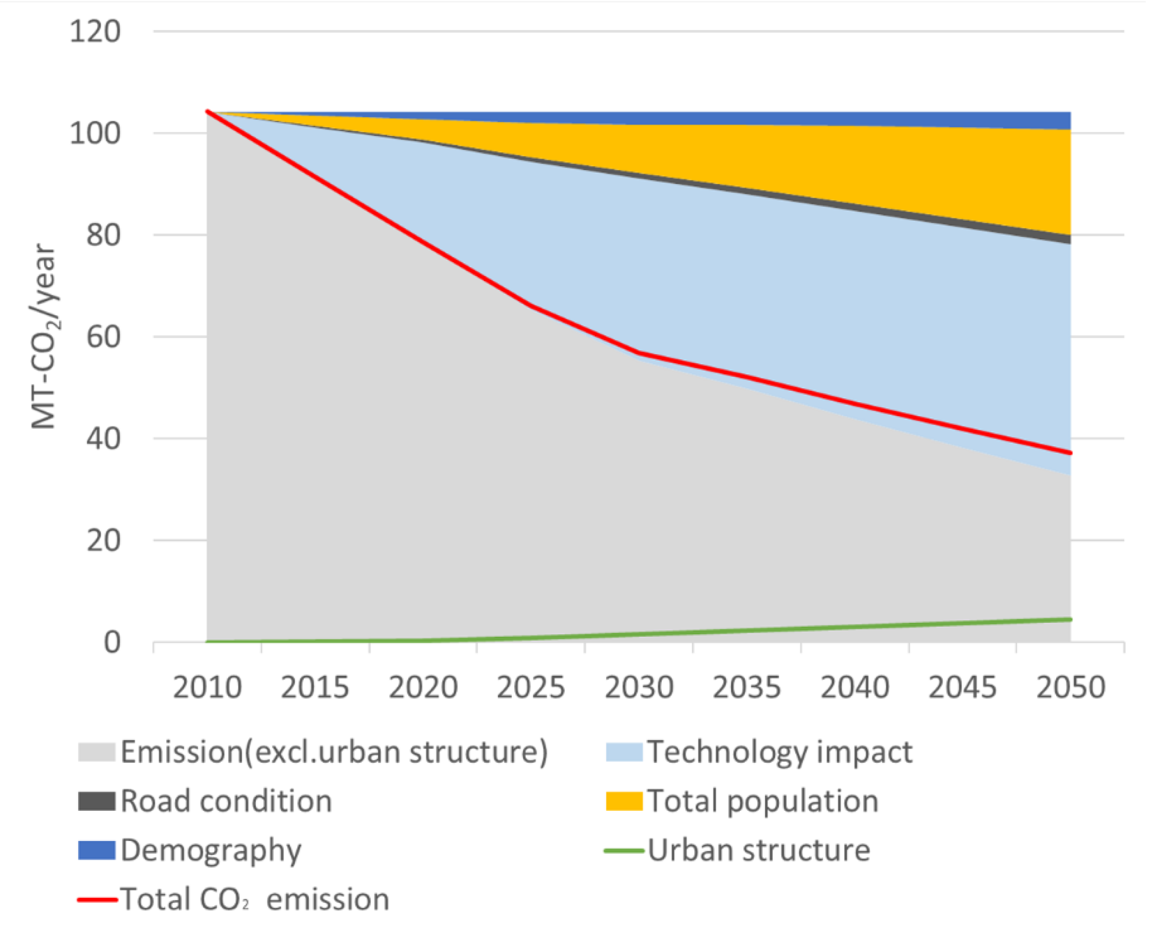
Figure 9 shows the estimated national total CO₂ emission from 2010 to 2050 and the contribution of various factors to emission changes. In the figure, the red line shows the trajectory of estimated total CO₂ emissions, which begin at 104 MTCO₂ in 2010 and are estimated to fall to 32.7 MTCO₂ in 2050, a 64% reduction. The technology factor contributes most to this decline, accounting for 43.6% of the reduction in emissions in 2050. The second largest contributor is the total population, which accounts for 19.7% of the emissions reduction, followed by demography, which contributes 3.4%. The urban structure factor, shown by the green line, is estimated to result in a 4.3% increase in total emissions. This means that, under the baseline scenario, suburbanization induces longer trips and greater car usage, both of which increase emissions. The dark gray area indicates the speed factor, which, by reducing congestion, decreases emissions by 1.9%.

Figure 10 shows the estimated CO₂ emissions and the contribution of the factors under the compact scenario. The total CO₂ emissions are estimated at 30.6 MTCO₂ in 2050, which is a 70% reduction from the 2010 level. The reduction rate under the compact scenario is 6% higher than that of the baseline scenario. In 2050, the technology factor contributes the largest share of this reduction at 40.6%, followed by the total population factor (17.8%), the urban structure (6.6%), the demography (3.1%), and the road speed factor (2.6%). Under the baseline scenario, the urban structure results in a 4.3% increase in emissions and, thus, the urban compaction scenario results in a substantial reduction in the emissions caused by the urban structure factor. Furthermore, the road speed factor reduces emissions more under the compact scenario than under the baseline scenario. In this study, urban compaction reduces the share of car usage and the vehicle travel length, while the road provision is assumed to be fixed. Therefore, there is less average lane traffic and a higher road speed under the compact scenario. It should be noted that the result would differ if urban compaction resulted in road traffic concentrating at certain links and inducing congestion.

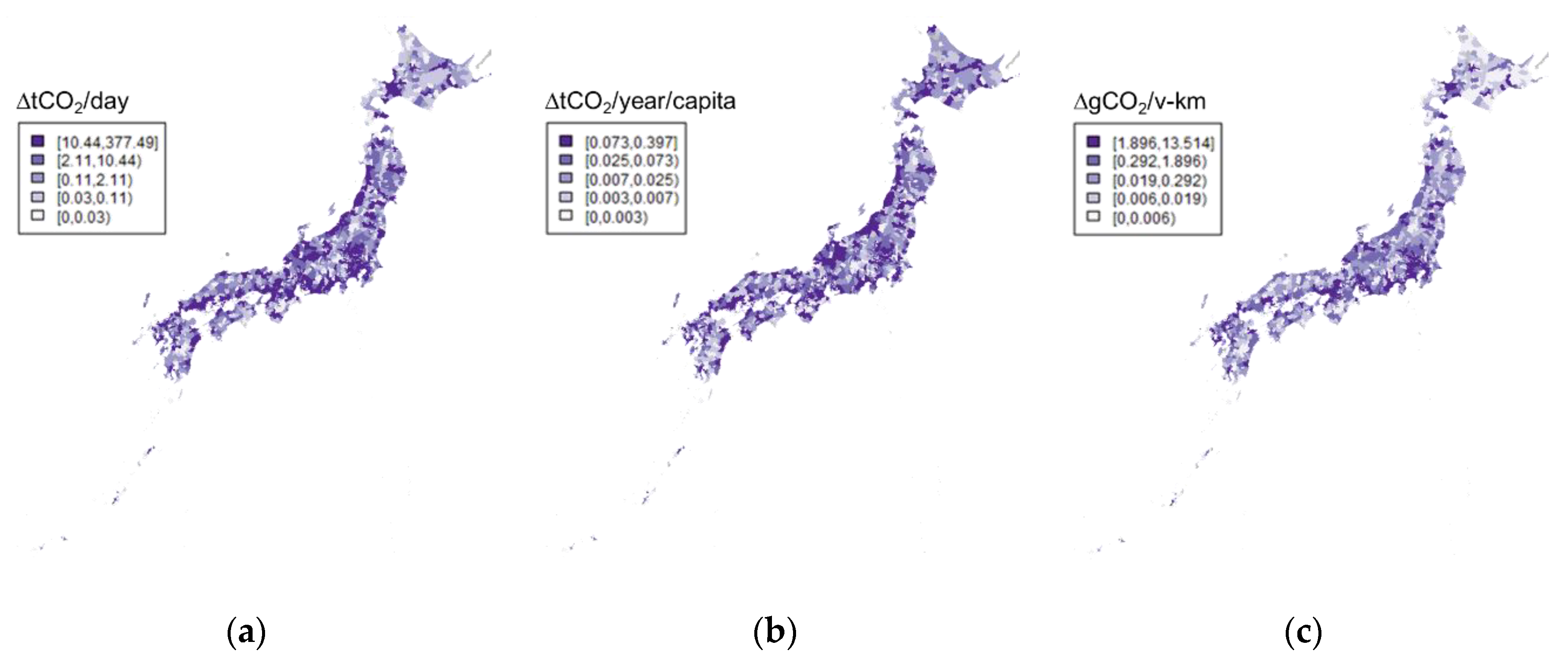
Figure 11 shows the change in the spatial distribution of CO₂ emissions under the baseline scenario between 2010 and 2050. The darker color indicates that the reduction in emissions is higher in the figure. The large cities and the small cities are shown to achieve large reductions in total CO₂ emissions, whereas municipalities in mountain areas have small reductions.

The municipalities in mountain areas have smaller populations and emit fewer emissions compared with urban municipalities in 2010, and the total volumes of emissions reduction is smaller in the future. The per capita reductions in volume of CO₂ emissions are smaller in large cities and larger in small cities. In small cities, the share of car usage is high, making the impact of emission reduction technologies high. Conversely, in large cities where the modal share of public transport is relatively high, the impact of automobile emission reduction technologies on per capita CO₂ emissions is relatively small. The volume of CO₂ emission reductions per vehicle-km is high in large cities. The road speed in large cities is relatively slow as a result of congestion and, therefore, technological improvements have a stronger effect in terms of reducing the absolute volume of emissions. At the same time, road speed will be faster and the emissions factor will be improved when traffic is reduced. Combined with these factors, the CO₂ emission per vehicle-km is reduced more in large cities than in small cities. In summary, the impact of CO₂ emission reduction differs by region, and different indices of emission changes correspond to different regional features. Details of these regional differences are provided in the Supplementary Materials.

Figure 12 shows the differences in the three indices between baseline and compact scenarios in 2050. The compact scenario derives lower CO₂ emissions than does the baseline scenario, and its impact is higher in large cities and lower in small cities. In other words, urban compaction is effective in reducing CO₂ emissions in urban areas but less effective in rural areas. The effect of urban compaction in reducing CO₂ emissions per capita is relatively weak at the center of large cities, but it is strong in local cities and in the suburbs of large cities. Population density in the center of large cities is already high, and the effect of urban compaction may be limited there. Local cities or suburbs of large cities have more capacity to reduce emissions per capita by urban compaction. The difference of emissions per vehicle-km indicates that urban compaction boosts reductions in emissions. In this study, urban compaction reduces the traffic volume by more than the baseline scenario and, as a result, traffic congestion is alleviated further. Therefore, the emissions per vehicle-km are reduced more in a compact scenario.

6. Discussion and Conclusions

In this study, we estimated that CO₂ emissions from passenger cars in 2050 are reduced by 64% and 70% under baseline and compact scenarios, respectively, compared with 2010 emissions. In 2016, the Japanese government set a long-term target of an 80% reduction in GHG emissions by 2050 in the Plan for Global Warming Countermeasures [34]. In this plan, the sectoral reduction targets are not determined. However, if we apply this target to passenger cars, an additional 10–14% reduction in emissions is required. Depopulation and aging in Japan reduce transport sector activities and consequently reduce CO₂ emissions, with the impact of these changes estimated to be about half of the reduction achieved via technological progress. To achieve the 2050 target, further emissions reduction measures are required.

We demonstrated that the expected population reduction will reduce the population density, which in turn will induce higher car dependency and longer car trip lengths. As a result, the urban structure factor increases the CO₂ emissions in the baseline scenario. Therefore, we need a measure to increase population density under the depopulating situation. As shown in our analysis, even an extremely drastic urban compaction scenario would reduce emissions by only 6%. This result clarifies that control of the urban space solely has a quite limited effect on CO₂ emissions reductions.

Reducing traffic volumes alleviates road congestion in the urban areas, which contributes to reducing CO₂ emissions, but the estimated impact is only 2%. In this study, urban compaction is estimated to reduce vehicle-kms and CO₂ emissions. However, if compaction and the resulting concentration of traffic aggravate congestion, then part of the emission reduction expected from urban compaction would not be achieved. Thus, urban compaction measures need to be combined with other countermeasures, including traffic control, land use management, and public transport provision, to alleviate road traffic concentration.

Our spatial analysis indicated that the per capita CO₂ emission reduction rate is higher for the local cities where the modal share of passenger cars is high. In these cities, improvements in automobile technologies will have a higher impact. The emission reduction effect of urban compaction is high in local cities and in the suburban municipalities of large cities but smaller at the center of large cities and very minor in municipalities in mountainous regions. These results indicate that the effects of emission reduction measures differ by regions. Therefore, the countermeasures of transport demand management should reflect regional features rather than applying uniform national measures. For instance, the combination of road speed improvements and road pricing to curb car traffic demand can be effective in reducing CO₂ emission in large cities. However, they may not be effective in small towns and low-density cities, where people are more dependent on cars and have fewer alternatives and therefore cannot change their travel behavior in response to these measures. In this case, road pricing simply increases user costs but may not reduce CO₂ emissions. Urban compaction may have a small effect in the center of large cities, which are already high density, and in mountainous areas, urban compaction has only a marginal effect owing to the sparse development patterns and low population density. Conversely, urban compaction in local cities or suburbs of large cities that have urban sprawl patterns will be effective in increasing population density and in reducing automobile dependency and car trip length. Demand management measures, including urban compaction policies, impose burdens on people to induce them to alter their behavior. Therefore, it is important to determine an effective framework for emission reduction measures that consider differences in impacts by regions.

In this study, we did not analyze the effect of a carbon intensity reduction by energy source and other demand side management measures, such as teleworking. The emissions factor for electricity is assumed to be fixed after 2030. If the share of renewable energy is increased substantially, then the emissions from using electricity will be reduced. As assumed in this study, if electric vehicles are widely disseminated, then a reduction in the emissions factor for electricity will have a considerable effect on CO₂ emissions from automobiles. Furthermore, if synthetic fuels derived from bioenergy or by a Fischer–Tropsch process can be delivered at a reasonable cost, then the internal combustion engine cars achieve zero well-to-wheel emissions. However, although these technologies may have a substantial impact, their progress is highly uncertain. Transport demand management measures such as teleworking and modal shifts, which may have a large impact on CO₂ emissions reductions, are not fully considered in this study because the feasibility of these measures is also very uncertain. Teleworking is becoming popular among private companies owing to the current infectious disease epidemic, but it is unclear whether this working style will continue. We need to carefully understand the impact of people’s behaviors, including their commuting patterns and location choices, that may affect travel behavior.

It should also be noted that our projections of car usage are based on the individual level, not the household level. Some studies use household-level projection because the purchase and the usage of cars are usually the decision by the household [38,39]. Household attributes, such as size, number of children, and income, affect the decision in purchasing cars and usage of cars, especially for accompanied travel. Households are composed of individuals, thus households have a wider variety of types than individuals. The projection of the future composition of household types for all municipalities is another big challenge. In Japan, depopulation and aging are expected to reduce the average household size, but it is unclear how the future shift of household composition affects car usage besides the aging of individual people. It should be addressed in future studies. Additionally, our demography scenario is based on IPSS and MLIT projections, which assumes a relatively conservative number of foreign immigrants (about 70 thousand net immigration annually in 2035). It is also possible to increase the foreign immigrants by the change of the Japanese immigration policy in the future, however, it is unpredictable. Our approach can be applied to the cases of the other demographic scenarios, and the increase of immigration will of course multiply the CO2 emission from passenger cars.

In summary, even with the assumption of substantial diffusion of CO₂ emissions reduction technologies, we find that the emissions reductions from passenger cars will not reach 80% in 2050. We need an additional 10–14% reduction to achieve the 80% target. In addition to the countermeasures considered in this study, we need to apply other measures to achieve the reduction target. There is no panacea of mitigation measures for climate change and all possible measures must be considered simultaneously. This maxim is also applicable in the CO₂ emissions reduction in the passenger car sector.

References

1. Sims, R.; Schaeffer, R.; Creutzig, F.; Cruz-Núñez, X.; D’Agosto, M.; Dimitriu, D.; Figueroa Meza, M.J.; Fulton, L.; Kobayashi, S.; Lah, O.; et al. Transport. In Climate Change 2014: Mitigation of Climate Change. Contribution of Working Group III to the Fifth Assessment Report of the Intergovernmental Panel on Climate Change; Edenhofer, O., Pichs-Madruga, R., Sokona, Y., Farahani, E., Kadner, S., Seyboth, K., Adler, A., Baum, I., Brunner, S., et al., Eds.; Cambridge University Press: Cambridge, UK, 2014; pp. 599–670. [Google Scholar]
2. Japan Automobile Manufacturers Association. Reducing CO2 Emissions in the Global Road Transport Sector. 2008. Available online: http://www.jama-english.jp/publications/2008_CO2_RoadTransport.pdf (accessed on 19 July 2020).
3. Creutzig, F.; Mühlhoff, R.; Römer, J. Decarbonizing urban transport in European cities: Four cases show possibly high co-benefits. Environ. Res. Lett. 2012, 7, 044042. [Google Scholar]
4. Pietzcker, R.; Longden, T.; Chen, W.; Fu, S.; Kriegler, E.; Kyle, P.; Luderer, G. Long-Term Transport Energy Demand and Climate Policy: Alternative Visions on Transport Decarbonization in Energy Economy Models. Energy 2014, 64, 95–108. [Google Scholar]
5. National Research Council. Transitions to Alternative Vehicles and Fuels; National Academies Press: Washington, DC, USA, 2013; p. 170. [Google Scholar]
6. European Environment Agency. Monitoring the CO2 Emissions from New Passenger Cars in the EU: Summary of Data for 2011; European Environment Agency: Copenhagen, Denmark, 2012. [Google Scholar]
7. Bandivadekar, A.; Bodek, K.; Cheah, L.; Evans, C.; Groode, T.; Heywood, J.; Kasseris, E.; Kromer, M.; Weiss, M. On the Road in 2035: Reducing Transportation’s Petroleum Consumption and GHG Emissions; Report No. LFEE 2008-05 RP; MIT Laboratory for Energy and the Environment: Cambridge, MA, USA, 2008; p. 196. Available online: http://web.mit.edu/sloan-auto-lab/research/beforeh2/otr2035/ (accessed on 19 July 2020).
8. Eads, G. 50by50 Prospects and Progress Report for Global Fuel Economy Initiative; Global Fuel Economy Initiative: London, UK, 2010; p. 64. Available online: https://www.globalfueleconomy.org/media/44119/50by50-prospects-and-progress-2011.pdf (accessed on 19 July 2020).
9. Kromer, M.A.; Heywood, J.B. Electric Powertrains: Opportunities and Challenges in the U.S. Light-Duty Vehicle Fleet; Massachusetts Institute of Technology: Cambridge, MA, USA, 2007; p. 157. Available online: http://web.mit.edu/sloan-auto-lab/research/beforeh2/files/kromer_electric_powertrains.pdf (accessed on 19 July 2020).
10. Greene, D.L.; Plotkin, S.E. Reducing Greenhouse Gas Emissions from U.S. Transportation; Pew Center on Global Climate Change: Arlington, VA, USA, 2011. [Google Scholar]
11. European Environment Agency. Monitoring CO2 Emissions from New Passenger Cars and Vans in 2017; European Environment Agency Report No. 15; Publications Office of the European Union: Luxembourg, 2019. [Google Scholar]
12. Barter, P.; Kenworthy, J.; Laube, F. Lessons from Asia on Sustainable Urban Transport. In Making Urban Transport Sustainable; Low, N., Gleeson, B., Eds.; Palgrave-Macmillan: Basingstoke, UK, 2003; pp. 252–270. [Google Scholar]
13. Litman, T. Parking Management: Strategies, Evaluation and Planning; Victoria Transport Policy Institute: Victoria, BC, Canada, 2016; Available online: https://www.vtpi.org/park_man.pdf (accessed on 19 July 2020).
14. Ribeiro, S.K.; Figueroa, M.J.; Creutzig, F.; Dubeux, C.; Hupe, J.; Kobayashi, S.; de Brettas, L.A.M.; Thrasher, T.; Webb, S.; Zou, J.; et al. Energy End-Use: Transport. In Global Energy Assessment: Toward a Sustainable Future; Johansson, T.B., Patwardhan, A., Nakicenovic, N., Gomez-Echeverri, L., Eds.; Cambridge University Press: Cambridge, UK, 2012; pp. 575–648. [Google Scholar]
15. Creutzig, F.; He, D. Climate change mitigation and co-benefits of feasible transport demand policies in Beijing. Transp. Res. Part D Transp. Environ. 2009, 14, 120–131. [Google Scholar]
16. Newman, P.; Kenworthy, J. The land use—transport connection. Land Use Policy 1996, 13, 1–22. [Google Scholar]
17. Cervero, R. Transit-Oriented Development in the United States: Experiences, Challenges, and Prospects; The National Academies Press: Washington, DC, USA, 2004. [Google Scholar]
18. Olaru, D.; Smith, B.; Taplin, J.H.E. Residential location and transit-oriented development in a new rail corridor. Transp. Res. Part A Policy Pr. 2011, 45, 219–237. [Google Scholar]
19. Banister, D. The sustainable mobility paradigm. Transp. Policy 2008, 15, 73–80. [Google Scholar]
20. Santos, G.; Behrendt, H.; Maconi, L.; Shirvani, T.; Teytelboym, A. Part I: Externalities and economic policies in road transport. Res. Transp. Econ. 2010, 28, 2–45. [Google Scholar]
21. Bongardt, D.; Creutzig, F.; Hüging, H.; Sakamoto, K.; Bakker, S.; Gota, S.; Böhler-Baedeker, S. Low-Carbon Land Transport: Policy Handbook; Routledge: New York, NY, USA, 2013; p. 264. [Google Scholar]
22. IEA. Energy Technology Perspectives; IEA: Paris, France, 2017; Available online: https://www.iea.org/reports/energy-technology-perspectives-2017 (accessed on 19 July 2020).
23. Cuenot, F.; Fulton, L.; Staub, J. The prospect for modal shifts in passenger transport worldwide and impacts on energy use and CO2. Energy Policy 2012, 41, 98–106. [Google Scholar]
24. Matsuhashi, K.; Ariga, T. Estimation of passenger car CO2 emissions with urban population density scenarios for low carbon transportation in Japan. IATSS Res. 2016, 39, 117–120. [Google Scholar]
25. Schipper, L.; Marie-Lilliu, C.; Gorham, R. Flexing the Link between Transport and Greenhouse Gas Emissions; International Energy Agency: Paris, France, 2000; p. 86. [Google Scholar]
26. Kamakaté, F.; Schipper, L. Trends in truck freight energy use and carbon emissions in selected OECD countries from 1973 to 2005. Energy Policy 2009, 37, 3743–3751. [Google Scholar]
27. Ministry of Land, Infrastructure and Transport of Japan. Results from the 4th Nationwide Person Trip Survey. Available online: https://www.mlit.go.jp/crd/tosiko/zpt/pdf/zenkokupt_gaiyouban_english.pdf (accessed on 18 July 2020).
28. National Land Information Division; National Spatial Planning and Regional Policy Bureau; Ministry of Land. Infrastructure and Transport of Japan, Kokudo Suuchi Jouhou. Available online: https://nlftp.mlit.go.jp/ksj/ (accessed on 18 July 2020). (In Japanese)
29. Ministry of Land, Infrastructure and Transport of Japan. National Road Census. Available online: https://www.mlit.go.jp/road/census/h27/index.html (accessed on 19 July 2020). (In Japanese)
30. National Institute of Population and Social Security Research. Population Projection for Japan: 2016–2065. 2017. Available online: http://www.ipss.go.jp/index-e.asp (accessed on 19 July 2020).
31. Ministry of Economy, Trade and Industry. Compilation of the Road Map for EVs and PHVs toward the Dissemination of Electric Vehicles and Plug-in Hybrid Vehicles. 2016. Available online: https://warp.da.ndl.go.jp/info:ndljp/pid/11253807/www.meti.go.jp/english/press/2016/0323_01.html (accessed on 19 July 2020).
32. Ministry of Economy, Trade and Industry. Formulation of a New Strategic Roadmap for Hydrogen and Fuel Cells. 2019. Available online: https://www.meti.go.jp/english/press/2019/0312_002.html (accessed on 19 July 2020).
33. International Energy Agency. Energy Technology Perspectives; IEA: Paris, France, 2012; Available online: https://www.iea.org/reports/energy-technology-perspectives-2012 (accessed on 19 July 2020).
34. Ministry of the Environment. Cabinet Decision on the Plan for Global Warming Countermeasures. 2016. Available online: https://www.env.go.jp/en/headline/2238.html (accessed on 19 July 2020).
35. Federation of Electric Power Companies of Japan. Addressing to Climate Change Issue Brief. 2015. Available online: https://www.fepc.or.jp/english/environment/annualreview/icsFiles/afieldfile/2016/03/01/actionplan_e_20151.pdf (accessed on 19 July 2020).
36. Namikawa, Y.; Takai, Y.; Ohshiro, N. Calculation Base of Motor Vehicle Emission Factors; Technical Note of National Institute of Land and Infrastructure Management; National Institute of Land and Infrastructure Management: Ibaraki, Japan, 2003. (In Japanese) [Google Scholar]
37. Ministry of the Environment. CO2 Emission Estimation Data for Transport Sector. Available online: https://www.env.go.jp/policy/local_keikaku/tools/car.html (accessed on 19 July 2020). (In Japanese)
38. Prskawetz, A.; Leiwen, J.; O’Neill, B.C. Demographic composition and projections of car use in Austria. Vienna Yearb. Popul. Res. 2004, 2, 175–201. [Google Scholar]
39. Meurs, H.; Haaijer, R.; Geurs, K.T. Modeling the effects of environmentally differentiated distance-based car-use charges in the Netherlands. Transp. Res. Part D Transp. Environ. 2013, 22, 1–9. [Google Scholar]
Figure 1. Analytical framework for the estimation of CO2 emissions from passenger cars.
Sustainability 12 06919 g001
Figure 2. Population trajectory in Japan (observed before 2015 using national census data, estimated after 2015 using National Institute of Population and Social Security Research (IPSS) data).
Sustainability 12 06919 g002
Figure 3. Example of a public transport catchment area.
Sustainability 12 06919 g003
Figure 4. Population distribution for 2010 and baseline and compact scenarios for 2050.
Sustainability 12 06919 g004
Figure 5. Automobile technology diffusion scenario (left: sales shares, right: shares of in-use vehicles).
Sustainability 12 06919 g005
Figure 6. CO2 emissions factor over the average travel speed by gasoline vehicles. Source: prepared by authors based on the Ministry of Land, Infrastructure, and Transport (MLIT) report.
Sustainability 12 06919 g006
Figure 7. Speed distribution of selected municipalities.
Sustainability 12 06919 g007
Figure 8. Relationship between lane traffic and log-normal distribution parameters (left: μ, right: σ).
Sustainability 12 06919 g008
Figure 9. Estimation of future CO2 emissions and contribution of the factors (the baseline scenario).
Sustainability 12 06919 g009
Figure 10. Estimation of future CO2 emissions and contribution of the factors (the compact scenario).
Sustainability 12 06919 g010
Figure 11. Differences in the spatial distribution of emission indices for 2010–2050 under the baseline scenario: (a) total CO2 emissions; (b) annual CO2 emissions per capita; and (c) CO2 emissions per vehicle-km.
Sustainability 12 06919 g011
Figure 12. Differences in emission indices between baseline and compact scenarios in 2050: (a) total CO2 emissions; (b) annual CO2 emissions per capita; (c) CO2 emissions per vehicle-km.
Sustainability 12 06919 g012