A Methodology to Increase the Accuracy of Particulate Matter Predictors Based on Time Decomposition


 ,
,  ,
,  ,
,  , and
, and
Abstract
:
1. Introduction
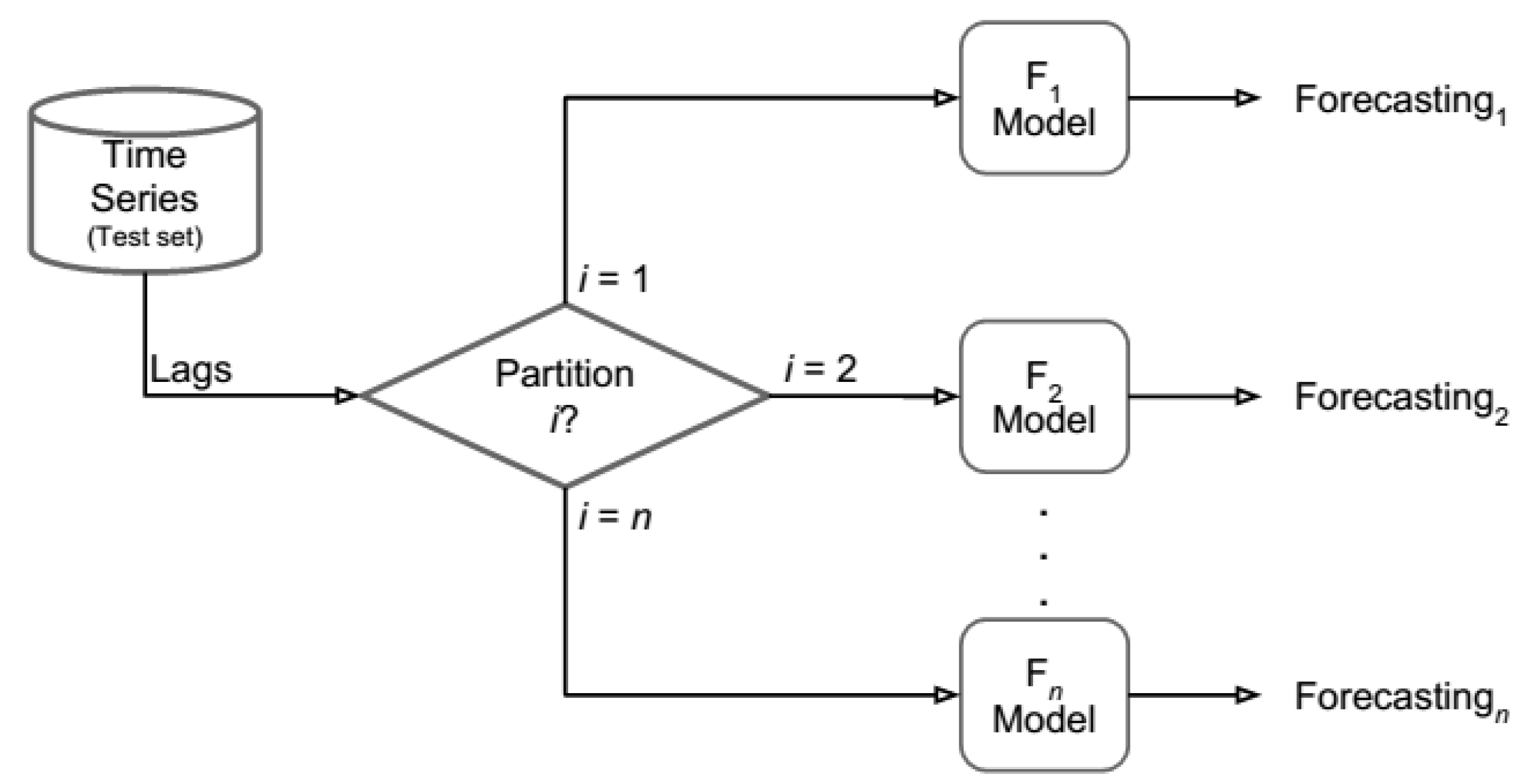
2. Proposed Methodology
- A seasonality test is conducted to find a suitable seasonal period for the series;
- The calculation of the CV is employed to determine which partitions present similar patterns;
- MLP, RBF, ESN, and ELM are used to assess the proposed methodology.
2.1. Partition Creation and Calculation of the Coefficient of Variation
2.2. Forecasting Models Used in the Proposed Approach
2.2.1. Multilayer Perceptron
- Input layer: transmits the input signal to the hidden layers;
- Hidden (intermediate) layers: these set of neurons performs a nonlinear transformation, mapping the input signal to another space;
- Output layer: this layer receives the signal from the hidden layers and generates a combination to form the network’s output. Often this process is based on linear combinations.
2.2.2. Radial Basis Function Network
2.2.3. Extreme Learning Machines
2.2.4. Echo State Networks
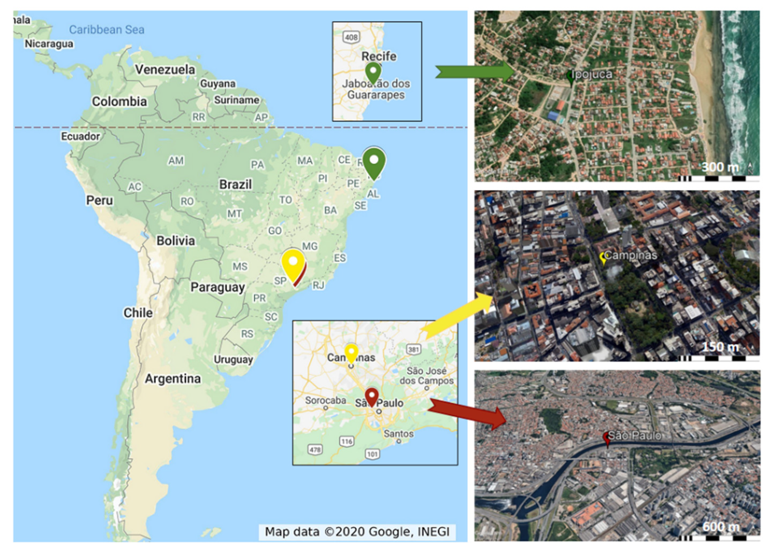
3. Case Studies
4. Computational Simulations
- Test set, for performance evaluation: it is composed of the last 10 samples of each month (for example, in January, we used the data from 22nd to 31st);
- Validation set, to avoid the excessive adjustment (only to the MLP): formed by the last 10 samples of the remainders of each month, excepting the test (in January, we used the data from 12nd to 21st);
- Training, to adjust the free parameters of the neural models: the remainder samples.
- Mean squared error (MSE):where is the observed sample in time t, is the prediction, and Ns the number of predicted samples.
- Mean absolute error (MAE):
- Mean absolute percentage error (MAPE):
- Root mean squared error (RMSE):
- Index of agreement (IA):in which is the average of the observed series.
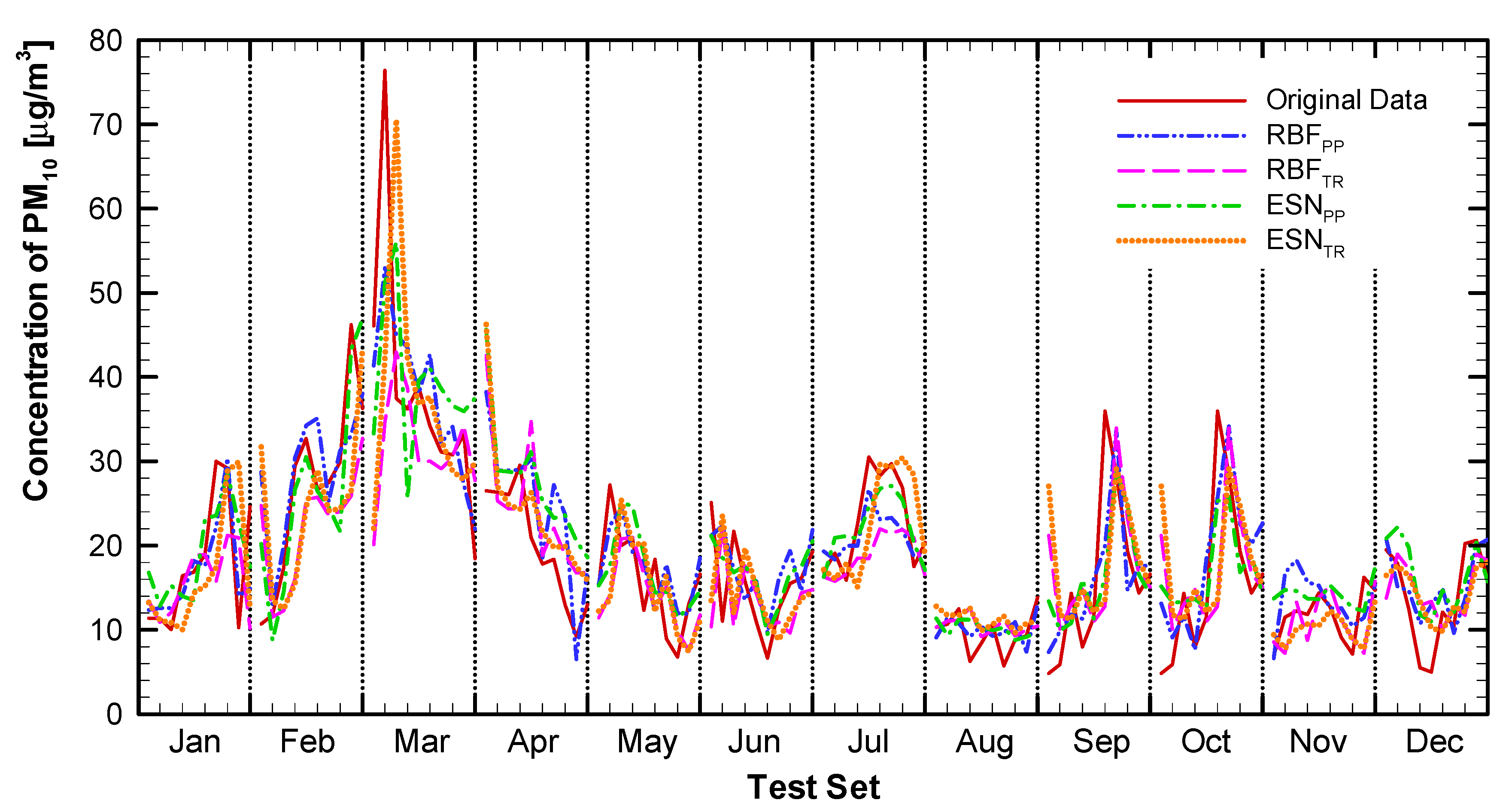
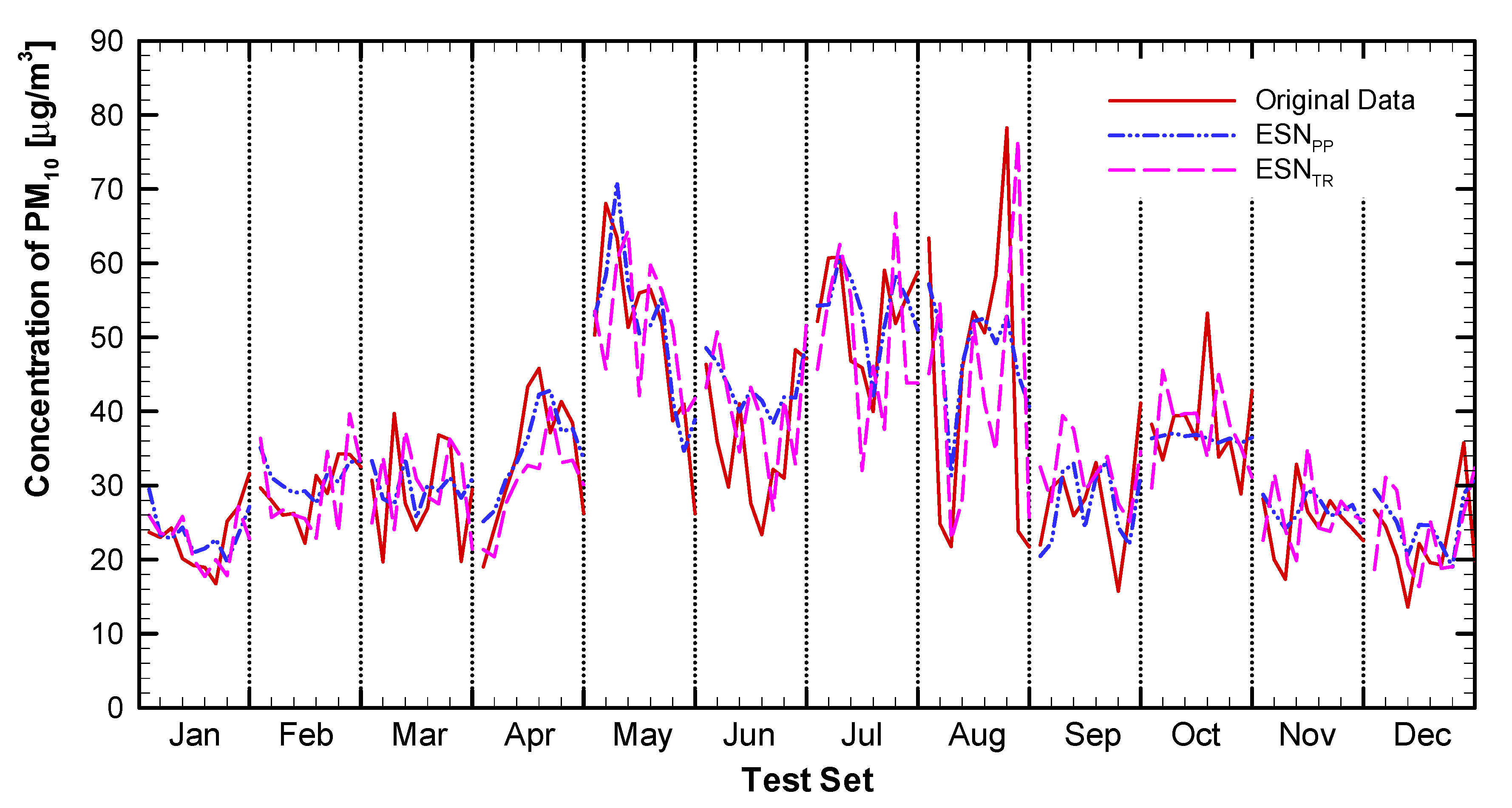
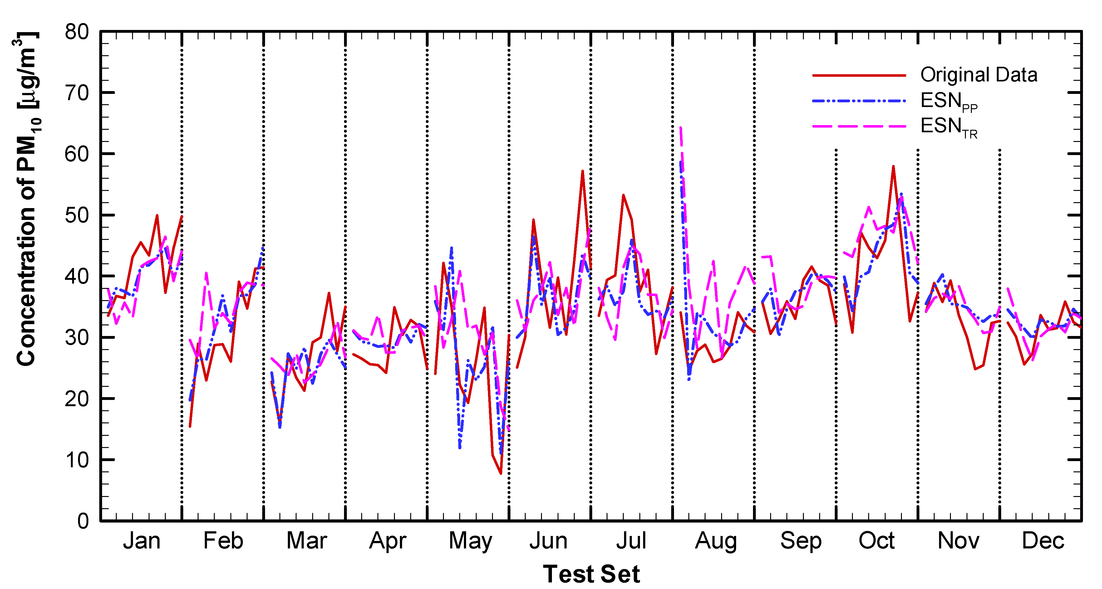
4.1. Results
4.2. Discussion
5. Conclusions
Author Contributions
Funding
Acknowledgments
Conflicts of Interest
Appendix A

| Metric | Jan | Feb | Mar | Apr | May | Jun | Jul | Aug | Sep | Oct | Nov | Dec | |
|---|---|---|---|---|---|---|---|---|---|---|---|---|---|
| MLPPP | MSE | 33.79 | 54.96 | 53.72 | 27.25 | 38.33 | 10.82 | 29.72 | 7.69 | 5.20 | 54.47 | 8.24 | 15.19 |
| MAE | 4.10 | 6.10 | 5.81 | 4.04 | 4.90 | 2.35 | 4.39 | 2.20 | 1.38 | 3.51 | 2.08 | 3.01 | |
| MAPE | 27.72 | 17.70 | 48.69 | 37.98 | 28.64 | 16.00 | 16.52 | 30.19 | 13.31 | 17.89 | 25.94 | 27.18 | |
| RMSE | 5.81 | 7.41 | 7.33 | 5.22 | 6.19 | 3.29 | 5.45 | 2.77 | 2.28 | 7.38 | 2.87 | 3.90 | |
| IA | 0.78 | 0.91 | 0.72 | 0.94 | 0.63 | 0.79 | 0.82 | 0.96 | 0.82 | 0.70 | 0.59 | 0.78 | |
| RBFPP | MSE | 21.41 | 35.13 | 38.06 | 24.47 | 30.08 | 9.08 | 31.14 | 4.65 | 4.73 | 34.21 | 6.83 | 15.68 |
| MAE | 3.44 | 5.49 | 4.60 | 3.94 | 4.03 | 2.30 | 4.28 | 1.90 | 1.82 | 3.65 | 2.11 | 3.46 | |
| MAPE | 20.86 | 18.45 | 24.54 | 35.91 | 23.76 | 17.03 | 18.69 | 21.11 | 14.08 | 18.57 | 22.68 | 39.49 | |
| RMSE | 4.63 | 5.93 | 6.17 | 4.95 | 5.48 | 3.01 | 5.58 | 2.16 | 2.18 | 5.85 | 2.61 | 3.96 | |
| IA | 0.86 | 0.96 | 0.88 | 0.94 | 0.73 | 0.83 | 0.88 | 0.98 | 0.89 | 0.87 | 0.79 | 0.74 | |
| ELMPP | MSE | 29.42 | 79.28 | 59.10 | 31.86 | 39.42 | 15.09 | 46.66 | 14.10 | 9.09 | 42.57 | 7.58 | 20.39 |
| MAE | 4.16 | 7.70 | 6.30 | 4.70 | 5.03 | 2.81 | 5.94 | 3.02 | 2.81 | 2.98 | 1.92 | 3.58 | |
| MAPE | 23.70 | 23.62 | 51.07 | 44.61 | 30.57 | 19.99 | 25.82 | 46.80 | 23.86 | 12.10 | 25.34 | 43.85 | |
| RMSE | 5.42 | 8.90 | 7.69 | 5.64 | 6.28 | 3.89 | 6.83 | 3.75 | 3.01 | 6.52 | 2.75 | 4.52 | |
| IA | 0.70 | 0.86 | 0.69 | 0.92 | 0.60 | 0.70 | 0.59 | 0.90 | 0.62 | 0.75 | 0.63 | 0.60 | |
| ESNPP | MSE | 23.59 | 56.50 | 45.52 | 32.84 | 27.31 | 8.88 | 37.14 | 7.57 | 5.24 | 36.39 | 7.48 | 16.81 |
| MAE | 3.87 | 6.50 | 5.42 | 4.89 | 4.40 | 2.36 | 4.61 | 2.18 | 1.60 | 2.85 | 1.95 | 3.24 | |
| MAPE | 25.60 | 19.90 | 49.98 | 41.49 | 23.37 | 17.60 | 23.06 | 32.30 | 14.20 | 15.61 | 24.98 | 39.44 | |
| RMSE | 4.86 | 7.52 | 6.75 | 5.73 | 5.23 | 2.98 | 6.09 | 2.75 | 2.29 | 6.03 | 2.74 | 4.10 | |
| IA | 0.78 | 0.92 | 0.78 | 0.93 | 0.78 | 0.81 | 0.81 | 0.96 | 0.85 | 0.81 | 0.65 | 0.69 | |
| ARPP | MSE | 24.37 | 33.48 | 76.04 | 30.05 | 34.31 | 11.86 | 37.25 | 11.61 | 8.16 | 41.06 | 7.27 | 20.95 |
| MAE | 3.60 | 4.98 | 6.98 | 4.59 | 5.09 | 2.64 | 4.54 | 2.61 | 2.29 | 4.33 | 1.88 | 3.73 | |
| MAPE | 26.18 | 15.20 | 67.26 | 36.45 | 33.53 | 22.09 | 27.20 | 35.93 | 20.58 | 32.84 | 23.64 | 43.16 | |
| RMSE | 4.94 | 5.79 | 8.72 | 5.48 | 5.86 | 3.44 | 6.10 | 3.41 | 2.86 | 6.41 | 2.70 | 4.58 | |
| IA | 0.80 | 0.96 | 0.58 | 0.95 | 0.73 | 0.78 | 0.85 | 0.94 | 0.78 | 0.79 | 0.71 | 0.57 | |
| MLPTR | MSE | 36.37 | 75.82 | 53.34 | 25.55 | 44.51 | 13.80 | 35.55 | 10.85 | 10.26 | 52.37 | 11.11 | 25.56 |
| MAE | 4.96 | 7.38 | 6.57 | 4.26 | 5.23 | 2.67 | 5.30 | 2.51 | 2.77 | 3.71 | 3.05 | 4.14 | |
| MAPE | 29.19 | 22.18 | 44.70 | 38.42 | 28.59 | 18.02 | 25.83 | 37.12 | 23.93 | 19.71 | 30.29 | 41.97 | |
| RMSE | 6.03 | 8.71 | 7.30 | 5.05 | 6.67 | 3.71 | 5.96 | 3.29 | 3.20 | 7.24 | 3.33 | 5.06 | |
| IA | 0.63 | 0.87 | 0.73 | 0.95 | 0.59 | 0.75 | 0.79 | 0.94 | 0.59 | 0.68 | 0.72 | 0.59 | |
| RBFTR | MSE | 38.82 | 78.13 | 46.95 | 22.37 | 47.54 | 15.40 | 32.90 | 12.90 | 12.28 | 57.20 | 13.45 | 26.61 |
| MAE | 5.03 | 7.49 | 6.45 | 4.00 | 5.03 | 2.86 | 4.81 | 2.83 | 3.12 | 3.83 | 3.37 | 4.29 | |
| MAPE | 29.45 | 22.51 | 41.27 | 35.57 | 27.14 | 20.14 | 23.87 | 42.50 | 26.45 | 19.06 | 32.94 | 44.71 | |
| RMSE | 6.23 | 8.84 | 6.85 | 4.73 | 6.89 | 3.92 | 5.74 | 3.59 | 3.50 | 7.56 | 3.67 | 5.16 | |
| IA | 0.62 | 0.86 | 0.79 | 0.95 | 0.55 | 0.72 | 0.82 | 0.92 | 0.53 | 0.68 | 0.67 | 0.51 | |
| ELMTR | MSE | 31.62 | 74.93 | 39.17 | 16.79 | 38.90 | 14.18 | 35.60 | 9.09 | 7.50 | 52.72 | 9.94 | 22.00 |
| MAE | 4.33 | 7.25 | 5.61 | 3.51 | 4.67 | 2.72 | 5.07 | 2.21 | 2.14 | 3.37 | 2.68 | 3.75 | |
| MAPE | 23.73 | 21.80 | 34.52 | 29.79 | 25.59 | 18.57 | 23.09 | 36.00 | 18.20 | 17.14 | 27.52 | 38.47 | |
| RMSE | 5.62 | 8.66 | 6.26 | 4.10 | 6.24 | 3.77 | 5.97 | 3.01 | 2.74 | 7.26 | 3.15 | 4.69 | |
| IA | 0.69 | 0.87 | 0.83 | 0.97 | 0.63 | 0.75 | 0.78 | 0.94 | 0.73 | 0.71 | 0.73 | 0.61 | |
| ESNTR | MSE | 31.48 | 76.61 | 49.01 | 22.46 | 51.36 | 14.15 | 33.70 | 11.19 | 7.93 | 54.40 | 10.39 | 22.07 |
| MAE | 4.19 | 7.51 | 6.39 | 3.84 | 5.87 | 2.61 | 4.82 | 2.70 | 2.60 | 4.04 | 2.66 | 3.77 | |
| MAPE | 26.05 | 22.73 | 39.04 | 35.03 | 31.75 | 17.53 | 23.21 | 40.63 | 21.91 | 21.78 | 26.34 | 42.46 | |
| RMSE | 5.61 | 8.75 | 7.00 | 4.74 | 7.17 | 3.76 | 5.81 | 3.35 | 2.82 | 7.38 | 3.22 | 4.70 | |
| IA | 0.75 | 0.87 | 0.81 | 0.95 | 0.59 | 0.77 | 0.81 | 0.93 | 0.69 | 0.68 | 0.73 | 0.62 | |
| ARTR | MSE | 103.18 | 116.57 | 173.42 | 107.56 | 113.79 | 33.00 | 51.40 | 23.00 | 20.84 | 83.75 | 32.82 | 27.27 |
| MAE | 8.24 | 9.50 | 11.50 | 8.56 | 8.84 | 4.27 | 6.02 | 3.63 | 4.02 | 5.03 | 4.74 | 4.34 | |
| MAPE | 37.94 | 25.70 | 57.66 | 52.68 | 32.98 | 22.49 | 30.27 | 56.51 | 36.02 | 24.16 | 29.04 | 46.94 | |
| RMSE | 10.16 | 10.80 | 13.17 | 10.37 | 10.67 | 5.74 | 7.17 | 4.80 | 4.57 | 9.15 | 5.73 | 5.22 | |
| IA | 0.83 | 0.90 | 0.88 | 0.58 | 0.86 | 0.88 | 0.83 | 0.84 | 0.51 | 0.72 | 0.87 | 0.65 | |
| PERS | MSE | 34.87 | 57.26 | 78.32 | 32.15 | 44.92 | 16.43 | 36.32 | 15.54 | 16.74 | 72.91 | 15.24 | 32.72 |
| MAE | 4.19 | 6.64 | 6.88 | 4.97 | 5.59 | 3.56 | 5.09 | 3.40 | 3.45 | 5.57 | 3.41 | 4.70 | |
| MAPE | 27.95 | 21.59 | 41.53 | 38.95 | 33.02 | 25.18 | 26.46 | 45.94 | 28.12 | 30.32 | 35.67 | 40.43 | |
| RMSE | 5.90 | 7.57 | 8.85 | 5.67 | 6.70 | 4.05 | 6.03 | 3.94 | 4.09 | 8.54 | 3.90 | 5.72 | |
| IA | 0.76 | 0.92 | 0.76 | 0.94 | 0.68 | 0.79 | 0.85 | 0.92 | 0.54 | 0.73 | 0.57 | 0.62 |
| Metric | Jan | Feb | Mar | Apr | May | Jun | Jul | Aug | Sep | Oct | Nov | Dec | |
|---|---|---|---|---|---|---|---|---|---|---|---|---|---|
| MLPPP | MSE | 6.41 | 13.51 | 29.91 | 12.90 | 7.03 | 1.76 | 14.24 | 1.32 | 2.55 | 32.71 | 0.99 | 14.01 |
| MAE | 1.75 | 2.99 | 4.23 | 2.22 | 2.17 | 1.08 | 3.28 | 0.91 | 1.32 | 3.28 | 0.84 | 3.21 | |
| MAPE | 21.69 | 17.09 | 46.94 | 19.36 | 30.25 | 19.27 | 20.73 | 19.70 | 19.68 | 44.55 | 13.94 | 81.17 | |
| RMSE | 2.53 | 3.68 | 5.47 | 3.59 | 2.65 | 1.33 | 3.77 | 1.15 | 1.60 | 5.72 | 0.99 | 3.74 | |
| IA | 0.91 | 0.95 | 0.47 | 0.81 | 0.56 | 0.85 | 0.78 | 0.98 | 0.87 | 0.70 | 0.86 | 0.49 | |
| RBFPP | MSE | 6.43 | 17.22 | 29.86 | 10.82 | 4.84 | 2.23 | 16.10 | 1.40 | 6.27 | 8.17 | 1.49 | 9.18 |
| MAE | 2.18 | 3.23 | 3.98 | 2.73 | 1.85 | 1.29 | 3.16 | 1.01 | 2.23 | 2.22 | 0.98 | 2.29 | |
| MAPE | 26.76 | 17.26 | 40.83 | 30.80 | 24.95 | 21.94 | 19.61 | 21.70 | 35.53 | 45.83 | 14.32 | 60.88 | |
| RMSE | 2.54 | 4.15 | 5.46 | 3.29 | 2.20 | 1.49 | 4.01 | 1.18 | 2.50 | 2.86 | 1.22 | 3.03 | |
| IA | 0.84 | 0.93 | 0.62 | 0.81 | 0.77 | 0.79 | 0.72 | 0.98 | 0.41 | 0.95 | 0.83 | 0.73 | |
| ELMPP | MSE | 5.06 | 25.50 | 27.43 | 18.22 | 6.95 | 3.63 | 12.08 | 3.41 | 7.69 | 33.36 | 1.94 | 16.64 |
| MAE | 1.95 | 4.17 | 3.83 | 3.31 | 2.26 | 1.51 | 2.97 | 1.39 | 2.13 | 3.13 | 1.11 | 3.56 | |
| MAPE | 25.47 | 27.13 | 45.15 | 32.67 | 30.41 | 28.04 | 18.33 | 34.90 | 32.29 | 45.73 | 18.97 | 87.76 | |
| RMSE | 2.25 | 5.05 | 5.24 | 4.27 | 2.64 | 1.90 | 3.48 | 1.85 | 2.77 | 5.78 | 1.39 | 4.08 | |
| IA | 0.90 | 0.90 | 0.44 | 0.65 | 0.61 | 0.57 | 0.85 | 0.94 | 0.50 | 0.70 | 0.65 | 0.42 | |
| ESNPP | MSE | 8.45 | 15.02 | 24.61 | 11.34 | 6.75 | 2.20 | 4.82 | 2.99 | 5.50 | 28.27 | 1.95 | 12.93 |
| MAE | 2.44 | 3.16 | 3.62 | 2.38 | 2.07 | 1.12 | 1.72 | 1.24 | 1.74 | 3.25 | 1.27 | 2.96 | |
| MAPE | 32.46 | 22.20 | 39.22 | 23.44 | 27.79 | 18.75 | 10.75 | 29.01 | 30.70 | 44.02 | 21.27 | 71.69 | |
| RMSE | 2.91 | 3.88 | 4.96 | 3.37 | 2.60 | 1.48 | 2.20 | 1.73 | 2.35 | 5.32 | 1.40 | 3.60 | |
| IA | 0.83 | 0.95 | 0.51 | 0.83 | 0.76 | 0.81 | 0.95 | 0.96 | 0.62 | 0.79 | 0.71 | 0.66 | |
| ARPP | MSE | 11.39 | 16.73 | 56.51 | 22.50 | 7.17 | 2.73 | 11.29 | 2.16 | 7.28 | 30.48 | 1.85 | 14.34 |
| MAE | 2.70 | 2.87 | 5.48 | 3.47 | 2.10 | 1.42 | 2.80 | 1.17 | 2.19 | 3.42 | 1.14 | 3.29 | |
| MAPE | 37.10 | 21.83 | 66.79 | 35.85 | 30.48 | 24.19 | 17.56 | 28.11 | 34.59 | 58.32 | 20.12 | 70.35 | |
| RMSE | 3.38 | 4.09 | 7.52 | 4.74 | 2.68 | 1.65 | 3.36 | 1.47 | 2.70 | 5.52 | 1.36 | 3.79 | |
| IA | 0.78 | 0.94 | 0.37 | 0.70 | 0.73 | 0.73 | 0.85 | 0.97 | 0.48 | 0.75 | 0.64 | 0.62 | |
| MLPTR | MSE | 9.35 | 36.07 | 43.18 | 20.21 | 7.58 | 4.09 | 20.30 | 2.58 | 9.59 | 37.35 | 2.12 | 20.92 |
| MAE | 2.35 | 5.20 | 4.58 | 3.37 | 2.04 | 1.73 | 3.44 | 1.27 | 2.41 | 3.44 | 0.90 | 4.13 | |
| MAPE | 26.07 | 31.45 | 53.36 | 32.38 | 23.56 | 27.21 | 20.62 | 31.77 | 34.39 | 46.31 | 12.54 | 94.29 | |
| RMSE | 3.06 | 6.01 | 6.57 | 4.50 | 2.75 | 2.02 | 4.51 | 1.61 | 3.10 | 6.11 | 1.45 | 4.57 | |
| IA | 0.80 | 0.83 | 0.42 | 0.65 | 0.54 | 0.73 | 0.68 | 0.95 | 0.44 | 0.68 | 0.77 | 0.42 | |
| RBFTR | MSE | 11.22 | 227.99 | 162.36 | 379.87 | 9748.12 | 3.76 | 29977.90 | 3.25 | 17.72 | 45.03 | 3.37 | 23.05 |
| MAE | 2.56 | 11.06 | 7.61 | 9.99 | 32.88 | 1.48 | 81.32 | 1.36 | 3.33 | 4.08 | 1.43 | 4.39 | |
| MAPE | 27.34 | 86.81 | 108.48 | 109.85 | 405.43 | 22.21 | 564.63 | 34.17 | 49.45 | 54.56 | 20.62 | 102.25 | |
| RMSE | 3.35 | 15.10 | 12.74 | 19.49 | 98.73 | 1.94 | 173.14 | 1.80 | 4.21 | 6.71 | 1.83 | 4.80 | |
| IA | 0.73 | 0.24 | 0.16 | 0.27 | 0.01 | 0.77 | 0.00 | 0.94 | 0.51 | 0.50 | 0.71 | 0.35 | |
| ELMTR | MSE | 4.95 | 31.75 | 42.73 | 17.92 | 7.33 | 3.56 | 12.72 | 2.23 | 8.06 | 34.14 | 2.15 | 18.79 |
| MAE | 1.95 | 4.72 | 4.63 | 2.87 | 2.03 | 1.58 | 3.00 | 1.16 | 2.27 | 3.10 | 0.96 | 3.86 | |
| MAPE | 21.98 | 29.21 | 53.01 | 25.83 | 23.95 | 24.33 | 19.16 | 29.37 | 33.43 | 45.43 | 13.52 | 89.46 | |
| RMSE | 2.23 | 5.64 | 6.54 | 4.23 | 2.71 | 1.89 | 3.57 | 1.50 | 2.84 | 5.84 | 1.47 | 4.34 | |
| IA | 0.88 | 0.88 | 0.41 | 0.68 | 0.66 | 0.76 | 0.83 | 0.96 | 0.49 | 0.71 | 0.81 | 0.47 | |
| ESNTR | MSE | 11.86 | 25.83 | 40.35 | 21.53 | 7.98 | 4.15 | 11.88 | 3.51 | 9.16 | 35.85 | 1.84 | 21.25 |
| MAE | 2.59 | 4.01 | 4.27 | 3.49 | 2.25 | 1.63 | 2.79 | 1.51 | 2.46 | 3.29 | 0.77 | 3.96 | |
| MAPE | 33.95 | 27.46 | 49.92 | 33.25 | 27.98 | 23.93 | 18.58 | 38.15 | 37.56 | 47.22 | 10.83 | 93.57 | |
| RMSE | 3.44 | 5.08 | 6.35 | 4.64 | 2.82 | 2.04 | 3.45 | 1.87 | 3.03 | 5.99 | 1.36 | 4.61 | |
| IA | 0.81 | 0.91 | 0.41 | 0.67 | 0.70 | 0.76 | 0.87 | 0.93 | 0.43 | 0.71 | 0.84 | 0.44 | |
| ARTR | MSE | 58.30 | 188.61 | 217.16 | 92.71 | 30.99 | 17.01 | 79.73 | 7.10 | 60.99 | 106.93 | 10.98 | 34.32 |
| MAE | 5.91 | 10.89 | 10.48 | 7.38 | 5.17 | 3.45 | 7.52 | 2.14 | 6.02 | 5.94 | 2.61 | 5.06 | |
| MAPE | 47.51 | 30.60 | 122.91 | 47.20 | 41.33 | 34.82 | 22.86 | 69.88 | 62.43 | 78.85 | 24.03 | 333.31 | |
| RMSE | 7.64 | 13.73 | 14.74 | 9.63 | 5.57 | 4.12 | 8.93 | 2.67 | 7.81 | 10.34 | 3.31 | 5.86 | |
| IA | 0.87 | 0.95 | 0.11 | 0.79 | 0.89 | 0.78 | 0.96 | 0.88 | 0.75 | 0.78 | 0.93 | 0.62 | |
| PERS | MSE | 16.40 | 22.77 | 67.26 | 29.09 | 9.08 | 4.76 | 16.15 | 3.02 | 14.46 | 44.13 | 2.47 | 33.33 |
| MAE | 2.73 | 3.90 | 6.05 | 4.00 | 2.54 | 1.72 | 3.31 | 1.48 | 2.98 | 4.57 | 1.18 | 4.87 | |
| MAPE | 32.16 | 28.30 | 75.79 | 41.74 | 33.83 | 28.28 | 22.63 | 33.82 | 48.57 | 66.59 | 18.14 | 93.74 | |
| RMSE | 4.05 | 4.77 | 8.20 | 5.39 | 3.01 | 2.18 | 4.02 | 1.74 | 3.80 | 6.64 | 1.57 | 5.77 | |
| IA | 0.78 | 0.93 | 0.33 | 0.63 | 0.62 | 0.66 | 0.83 | 0.96 | 0.43 | 0.75 | 0.72 | 0.43 |
| Metric | Jan | Feb | Mar | Apr | May | Jun | Jul | Aug | Sep | Oct | Nov | Dec | |
|---|---|---|---|---|---|---|---|---|---|---|---|---|---|
| MLPPP | MSE | 42.06 | 76.13 | 75.64 | 30.58 | 27.42 | 23.16 | 17.79 | 6.40 | 74.74 | 73.58 | 16.43 | 22.69 |
| MAE | 5.05 | 6.36 | 6.55 | 4.70 | 4.39 | 3.68 | 3.37 | 1.93 | 6.03 | 6.09 | 3.39 | 4.21 | |
| MAPE | 28.39 | 30.44 | 15.77 | 28.15 | 38.05 | 29.09 | 14.31 | 23.03 | 52.15 | 57.99 | 36.69 | 37.35 | |
| RMSE | 6.49 | 8.73 | 8.70 | 5.53 | 5.24 | 4.81 | 4.22 | 2.53 | 8.65 | 8.58 | 4.05 | 4.76 | |
| IA | 0.58 | 0.78 | 0.90 | 0.96 | 0.77 | 0.61 | 0.78 | 0.98 | 0.69 | 0.62 | 0.75 | 0.83 | |
| RBFPP | MSE | 18.75 | 59.08 | 80.90 | 45.65 | 22.84 | 23.91 | 14.08 | 4.33 | 37.84 | 35.48 | 12.67 | 17.96 |
| MAE | 3.21 | 5.15 | 6.60 | 5.42 | 4.02 | 4.06 | 3.28 | 1.79 | 4.71 | 5.17 | 2.88 | 3.50 | |
| MAPE | 17.96 | 28.04 | 15.92 | 30.75 | 31.83 | 31.63 | 13.99 | 23.34 | 31.36 | 45.27 | 25.87 | 39.08 | |
| RMSE | 4.33 | 7.69 | 8.99 | 6.76 | 4.78 | 4.89 | 3.75 | 2.08 | 6.15 | 5.96 | 3.56 | 4.24 | |
| IA | 0.88 | 0.89 | 0.88 | 0.94 | 0.81 | 0.72 | 0.83 | 0.98 | 0.84 | 0.87 | 0.87 | 0.82 | |
| ELMPP | MSE | 47.77 | 86.75 | 180.87 | 68.37 | 20.55 | 25.88 | 21.18 | 11.39 | 75.77 | 75.67 | 7.85 | 27.25 |
| MAE | 5.45 | 6.73 | 8.84 | 6.69 | 3.68 | 4.14 | 3.46 | 2.20 | 5.62 | 5.54 | 2.57 | 4.35 | |
| MAPE | 31.24 | 32.82 | 22.98 | 39.09 | 28.37 | 35.37 | 14.47 | 31.01 | 51.98 | 52.45 | 24.10 | 49.00 | |
| RMSE | 6.91 | 9.31 | 13.45 | 8.27 | 4.53 | 5.09 | 4.60 | 3.38 | 8.70 | 8.70 | 2.80 | 5.22 | |
| IA | 0.53 | 0.78 | 0.62 | 0.90 | 0.86 | 0.58 | 0.80 | 0.95 | 0.69 | 0.68 | 0.92 | 0.70 | |
| ESNPP | MSE | 34.15 | 31.77 | 176.27 | 83.43 | 25.28 | 13.41 | 9.92 | 7.13 | 59.59 | 34.95 | 14.92 | 17.91 |
| MAE | 4.21 | 4.52 | 10.58 | 7.54 | 4.06 | 2.98 | 2.55 | 1.99 | 5.45 | 4.83 | 2.95 | 3.45 | |
| MAPE | 29.16 | 17.82 | 28.85 | 46.04 | 30.34 | 22.84 | 11.30 | 25.34 | 48.74 | 43.30 | 32.54 | 38.72 | |
| RMSE | 5.84 | 5.64 | 13.28 | 9.13 | 5.03 | 3.66 | 3.15 | 2.67 | 7.72 | 5.91 | 3.86 | 4.23 | |
| IA | 0.80 | 0.95 | 0.75 | 0.87 | 0.81 | 0.81 | 0.91 | 0.97 | 0.72 | 0.82 | 0.78 | 0.82 | |
| ARPP | MSE | 48.33 | 74.74 | 199.81 | 58.92 | 31.84 | 44.52 | 10.63 | 8.01 | 84.54 | 84.54 | 15.19 | 26.91 |
| MAE | 5.41 | 6.18 | 10.70 | 5.59 | 4.37 | 5.39 | 2.66 | 2.14 | 6.66 | 6.66 | 3.22 | 4.10 | |
| MAPE | 34.39 | 30.93 | 32.54 | 26.61 | 35.15 | 40.44 | 12.53 | 27.62 | 73.17 | 73.17 | 32.47 | 43.21 | |
| RMSE | 6.95 | 8.65 | 14.14 | 7.68 | 5.64 | 6.67 | 3.26 | 2.83 | 9.19 | 9.19 | 3.90 | 5.19 | |
| IA | 0.61 | 0.84 | 0.68 | 0.94 | 0.70 | 0.47 | 0.91 | 0.97 | 0.53 | 0.53 | 0.80 | 0.73 | |
| MLPTR | MSE | 60.01 | 107.66 | 260.43 | 38.51 | 34.04 | 40.02 | 26.00 | 7.54 | 75.85 | 75.85 | 9.72 | 21.69 |
| MAE | 5.45 | 7.82 | 11.27 | 4.98 | 4.95 | 5.12 | 4.28 | 1.81 | 5.59 | 5.59 | 2.15 | 4.01 | |
| MAPE | 30.03 | 34.39 | 27.31 | 29.65 | 31.94 | 33.95 | 18.00 | 24.54 | 55.45 | 55.45 | 18.04 | 39.34 | |
| RMSE | 7.75 | 10.38 | 16.14 | 6.21 | 5.83 | 6.33 | 5.10 | 2.75 | 8.71 | 8.71 | 3.12 | 4.66 | |
| IA | 0.53 | 0.68 | 0.45 | 0.95 | 0.80 | 0.60 | 0.69 | 0.97 | 0.62 | 0.62 | 0.93 | 0.80 | |
| RBFTR | MSE | 58.16 | 84.31 | 242.66 | 59.80 | 23.17 | 56.10 | 30.12 | 8.30 | 90.22 | 90.22 | 12.79 | 21.92 |
| MAE | 5.45 | 6.63 | 9.74 | 5.97 | 3.96 | 6.00 | 4.40 | 1.87 | 6.50 | 6.50 | 2.71 | 4.04 | |
| MAPE | 29.81 | 29.83 | 21.02 | 33.69 | 27.49 | 39.76 | 17.58 | 25.62 | 62.21 | 62.21 | 23.07 | 41.10 | |
| RMSE | 7.63 | 9.18 | 15.58 | 7.73 | 4.81 | 7.49 | 5.49 | 2.88 | 9.50 | 9.50 | 3.58 | 4.68 | |
| IA | 0.56 | 0.77 | 0.41 | 0.92 | 0.85 | 0.46 | 0.59 | 0.96 | 0.62 | 0.62 | 0.90 | 0.79 | |
| ELMTR | MSE | 138.81 | 77.37 | 1208.77 | 35.64 | 98.83 | 78.60 | 143.61 | 7.13 | 88.22 | 88.22 | 15.82 | 13.04 |
| MAE | 8.77 | 7.01 | 21.17 | 4.09 | 8.59 | 6.34 | 9.29 | 1.81 | 6.45 | 6.45 | 3.09 | 2.95 | |
| MAPE | 50.80 | 27.96 | 74.37 | 24.01 | 57.49 | 45.14 | 40.00 | 23.81 | 67.45 | 67.45 | 28.01 | 27.19 | |
| RMSE | 11.78 | 8.80 | 34.77 | 5.97 | 9.94 | 8.87 | 11.98 | 2.67 | 9.39 | 9.39 | 3.98 | 3.61 | |
| IA | 0.48 | 0.79 | 0.32 | 0.96 | 0.65 | 0.59 | 0.66 | 0.97 | 0.61 | 0.61 | 0.89 | 0.89 | |
| ESNTR | MSE | 71.34 | 115.27 | 239.23 | 50.10 | 44.84 | 49.51 | 25.52 | 8.67 | 98.79 | 98.79 | 11.26 | 20.20 |
| MAE | 5.87 | 8.44 | 10.93 | 5.27 | 5.81 | 6.07 | 3.74 | 2.07 | 6.67 | 6.67 | 2.50 | 3.79 | |
| MAPE | 37.37 | 38.91 | 28.02 | 30.08 | 38.71 | 41.80 | 17.33 | 27.85 | 71.10 | 71.10 | 20.29 | 40.06 | |
| RMSE | 8.45 | 10.74 | 15.47 | 7.08 | 6.70 | 7.04 | 5.05 | 2.94 | 9.94 | 9.94 | 3.36 | 4.49 | |
| IA | 0.60 | 0.76 | 0.66 | 0.94 | 0.75 | 0.50 | 0.83 | 0.96 | 0.55 | 0.55 | 0.92 | 0.80 | |
| ARTR | MSE | 340.26 | 390.36 | 1562.82 | 223.77 | 170.67 | 176.45 | 126.24 | 29.43 | 158.63 | 158.63 | 36.32 | 43.24 |
| MAE | 14.14 | 15.08 | 28.68 | 12.33 | 11.01 | 10.87 | 8.66 | 3.90 | 8.53 | 8.53 | 4.66 | 5.70 | |
| MAPE | 52.31 | 44.46 | 34.82 | 48.39 | 35.63 | 50.34 | 19.68 | 63.15 | 218.30 | 218.30 | 23.13 | 59.52 | |
| RMSE | 18.45 | 19.76 | 39.53 | 14.96 | 13.06 | 13.28 | 11.24 | 5.42 | 12.59 | 12.59 | 6.03 | 6.58 | |
| IA | 0.81 | 0.89 | 0.89 | 0.65 | 0.89 | 0.69 | 0.96 | 0.86 | 0.58 | 0.58 | 0.84 | 0.69 | |
| PERS | MSE | 73.55 | 105.38 | 332.57 | 56.22 | 46.08 | 58.54 | 23.38 | 10.83 | 135.86 | 135.86 | 13.34 | 29.02 |
| MAE | 5.70 | 7.89 | 12.35 | 4.94 | 5.93 | 6.44 | 3.91 | 2.73 | 8.93 | 8.93 | 2.67 | 4.43 | |
| MAPE | 36.23 | 38.82 | 32.03 | 26.35 | 41.46 | 45.73 | 18.04 | 33.70 | 82.36 | 82.36 | 22.24 | 37.55 | |
| RMSE | 8.58 | 10.27 | 18.24 | 7.50 | 6.79 | 7.65 | 4.84 | 3.29 | 11.66 | 11.66 | 3.65 | 5.39 | |
| IA | 0.62 | 0.80 | 0.56 | 0.94 | 0.73 | 0.46 | 0.84 | 0.96 | 0.59 | 0.59 | 0.90 | 0.80 |
| Metric | Jan | Feb | Mar | Apr | May | Jun | Jul | Aug | Sep | Oct | Nov | Dec | |
|---|---|---|---|---|---|---|---|---|---|---|---|---|---|
| MLPPP | MSE | 83.18 | 25.43 | 35.11 | 40.66 | 88.37 | 86.17 | 96.45 | 75.08 | 226.37 | 19.76 | 55.82 | 18.78 |
| MAE | 8.08 | 4.58 | 4.75 | 4.72 | 7.63 | 8.20 | 8.54 | 7.87 | 8.88 | 2.87 | 6.13 | 3.06 | |
| MAPE | 24.78 | 17.86 | 20.37 | 13.93 | 27.07 | 17.34 | 18.34 | 32.28 | 85.16 | 9.70 | 22.85 | 17.52 | |
| RMSE | 9.12 | 5.04 | 5.93 | 6.38 | 9.40 | 9.28 | 9.82 | 8.66 | 15.05 | 4.45 | 7.47 | 4.33 | |
| IA | 0.84 | 0.71 | 0.87 | 0.95 | 0.84 | 0.85 | 0.87 | 0.95 | 0.86 | 0.93 | 0.61 | 0.77 | |
| RBFPP | MSE | 99.12 | 7.27 | 34.05 | 43.42 | 78.31 | 98.97 | 39.80 | 61.14 | 370.70 | 25.03 | 38.71 | 9.96 |
| MAE | 8.19 | 2.15 | 4.54 | 5.68 | 7.22 | 7.66 | 5.33 | 6.57 | 11.99 | 3.98 | 5.08 | 2.76 | |
| MAPE | 23.26 | 7.64 | 20.21 | 17.16 | 22.83 | 17.66 | 9.88 | 26.51 | 133.30 | 11.65 | 18.38 | 15.01 | |
| RMSE | 9.96 | 2.70 | 5.84 | 6.59 | 8.85 | 9.95 | 6.31 | 7.82 | 19.25 | 5.00 | 6.22 | 3.16 | |
| IA | 0.76 | 0.92 | 0.81 | 0.92 | 0.85 | 0.81 | 0.95 | 0.96 | 0.72 | 0.87 | 0.64 | 0.90 | |
| ELMPP | MSE | 88.20 | 16.73 | 34.62 | 62.27 | 107.28 | 93.21 | 101.08 | 135.57 | 241.65 | 27.67 | 51.69 | 16.74 |
| MAE | 8.21 | 3.37 | 4.12 | 6.17 | 8.98 | 8.06 | 8.51 | 10.38 | 10.72 | 3.78 | 6.20 | 3.02 | |
| MAPE | 24.44 | 13.69 | 14.91 | 17.48 | 32.09 | 21.22 | 15.26 | 40.43 | 108.52 | 10.73 | 22.04 | 17.21 | |
| RMSE | 9.39 | 4.09 | 5.88 | 7.89 | 10.36 | 9.65 | 10.05 | 11.64 | 15.55 | 5.26 | 7.19 | 4.09 | |
| IA | 0.82 | 0.73 | 0.81 | 0.86 | 0.78 | 0.82 | 0.88 | 0.89 | 0.82 | 0.86 | 0.64 | 0.77 | |
| ESNPP | MSE | 73.61 | 9.31 | 21.02 | 68.25 | 87.18 | 96.13 | 71.79 | 39.88 | 260.88 | 48.37 | 35.96 | 15.69 |
| MAE | 7.18 | 2.58 | 3.66 | 6.89 | 7.12 | 8.75 | 6.71 | 5.12 | 10.70 | 5.61 | 4.61 | 2.87 | |
| MAPE | 21.37 | 11.62 | 14.34 | 19.26 | 28.41 | 19.03 | 13.34 | 18.49 | 96.85 | 16.38 | 17.52 | 16.72 | |
| RMSE | 8.58 | 3.05 | 4.58 | 8.26 | 9.34 | 9.80 | 8.47 | 6.32 | 16.15 | 6.95 | 6.00 | 3.96 | |
| IA | 0.87 | 0.91 | 0.90 | 0.88 | 0.88 | 0.81 | 0.92 | 0.97 | 0.80 | 0.68 | 0.72 | 0.79 | |
| ARPP | MSE | 75.76 | 13.27 | 25.09 | 81.89 | 95.36 | 131.43 | 126.04 | 103.74 | 304.84 | 46.40 | 39.04 | 17.09 |
| MAE | 7.61 | 2.66 | 3.88 | 6.70 | 7.83 | 9.90 | 9.85 | 8.58 | 11.67 | 5.40 | 5.20 | 3.51 | |
| MAPE | 24.57 | 12.03 | 15.83 | 20.27 | 31.44 | 22.02 | 19.94 | 38.09 | 110.48 | 15.74 | 19.27 | 18.95 | |
| RMSE | 8.70 | 3.64 | 5.01 | 9.05 | 9.77 | 11.46 | 11.23 | 10.19 | 17.46 | 6.81 | 6.25 | 4.13 | |
| IA | 0.86 | 0.83 | 0.87 | 0.83 | 0.85 | 0.74 | 0.85 | 0.92 | 0.79 | 0.67 | 0.67 | 0.84 | |
| MLPTR | MSE | 115.94 | 27.97 | 31.68 | 139.21 | 125.65 | 136.33 | 231.53 | 170.03 | 284.37 | 120.30 | 100.27 | 17.80 |
| MAE | 9.42 | 4.44 | 4.53 | 10.11 | 9.42 | 8.27 | 13.52 | 11.16 | 10.91 | 8.13 | 8.68 | 3.75 | |
| MAPE | 29.88 | 17.28 | 17.92 | 27.95 | 34.94 | 16.91 | 24.17 | 45.27 | 109.31 | 23.71 | 32.66 | 19.73 | |
| RMSE | 10.77 | 5.29 | 5.63 | 11.80 | 11.21 | 11.68 | 15.22 | 13.04 | 16.86 | 10.97 | 10.01 | 4.22 | |
| IA | 0.78 | 0.58 | 0.86 | 0.69 | 0.77 | 0.68 | 0.62 | 0.86 | 0.79 | 0.28 | 0.46 | 0.85 | |
| RBFTR | MSE | 133.41 | 26.47 | 70.20 | 119.44 | 192.56 | 225.62 | 256.58 | 180.61 | 316.18 | 98.14 | 103.74 | 16.50 |
| MAE | 10.03 | 4.44 | 7.17 | 9.86 | 12.34 | 14.26 | 14.40 | 11.16 | 10.63 | 7.61 | 8.87 | 3.36 | |
| MAPE | 29.25 | 17.18 | 28.39 | 28.42 | 42.87 | 32.88 | 26.20 | 37.63 | 108.96 | 21.48 | 32.18 | 17.88 | |
| RMSE | 11.55 | 5.14 | 8.38 | 10.93 | 13.88 | 15.02 | 16.02 | 13.44 | 17.78 | 9.91 | 10.19 | 4.06 | |
| IA | 0.75 | 0.55 | 0.67 | 0.74 | 0.61 | 0.35 | 0.62 | 0.85 | 0.82 | 0.18 | 0.21 | 0.85 | |
| ELMTR | MSE | 124.15 | 28.85 | 32.10 | 135.68 | 118.77 | 125.79 | 207.64 | 151.44 | 266.64 | 110.73 | 92.64 | 14.38 |
| MAE | 9.52 | 4.66 | 4.69 | 9.68 | 9.56 | 7.50 | 12.94 | 10.57 | 8.93 | 7.55 | 8.25 | 3.41 | |
| MAPE | 30.23 | 18.24 | 18.23 | 27.39 | 33.14 | 13.98 | 23.75 | 42.93 | 96.96 | 21.75 | 31.15 | 17.45 | |
| RMSE | 11.14 | 5.37 | 5.67 | 11.65 | 10.90 | 11.22 | 14.41 | 12.31 | 16.33 | 10.52 | 9.62 | 3.79 | |
| IA | 0.77 | 0.61 | 0.86 | 0.71 | 0.79 | 0.75 | 0.64 | 0.88 | 0.83 | 0.34 | 0.50 | 0.89 | |
| ESNTR | MSE | 102.98 | 13.89 | 28.01 | 136.71 | 150.38 | 171.41 | 220.79 | 172.95 | 270.97 | 74.31 | 103.01 | 15.37 |
| MAE | 8.76 | 2.54 | 4.72 | 10.27 | 10.02 | 9.90 | 13.03 | 10.87 | 11.38 | 7.23 | 8.57 | 3.40 | |
| MAPE | 27.63 | 11.45 | 18.99 | 32.07 | 36.30 | 26.95 | 23.57 | 38.10 | 100.18 | 22.06 | 33.02 | 17.28 | |
| RMSE | 10.15 | 3.73 | 5.29 | 11.69 | 12.26 | 13.09 | 14.86 | 13.15 | 16.46 | 8.62 | 10.15 | 3.92 | |
| IA | 0.83 | 0.85 | 0.91 | 0.75 | 0.70 | 0.74 | 0.64 | 0.85 | 0.80 | 0.58 | 0.45 | 0.86 | |
| ARTR | MSE | 138.64 | 52.17 | 55.57 | 191.96 | 221.42 | 306.05 | 496.17 | 408.73 | 562.43 | 189.19 | 174.39 | 26.71 |
| MAE | 10.32 | 5.87 | 6.34 | 11.21 | 12.49 | 14.78 | 20.53 | 16.81 | 15.68 | 10.87 | 11.37 | 4.31 | |
| MAPE | 30.28 | 17.99 | 17.57 | 28.68 | 38.44 | 22.41 | 27.07 | 75.76 | 89.67 | 24.01 | 32.63 | 17.18 | |
| RMSE | 11.77 | 7.22 | 7.45 | 13.86 | 14.88 | 17.49 | 22.27 | 20.22 | 23.72 | 13.75 | 13.21 | 5.17 | |
| IA | 0.86 | 0.91 | 0.93 | 0.83 | 0.84 | 0.95 | 0.88 | 0.81 | 0.48 | 0.85 | 0.78 | 0.79 | |
| PERS | MSE | 131.44 | 32.44 | 60.26 | 148.14 | 215.47 | 183.56 | 231.51 | 127.88 | 435.96 | 138.17 | 119.08 | 21.86 |
| MAE | 10.30 | 5.25 | 6.82 | 9.86 | 12.06 | 11.67 | 12.01 | 8.97 | 12.57 | 8.74 | 8.64 | 3.81 | |
| MAPE | 33.01 | 20.60 | 30.08 | 29.94 | 48.25 | 29.56 | 24.08 | 29.47 | 117.95 | 27.07 | 35.06 | 20.77 | |
| RMSE | 11.46 | 5.70 | 7.76 | 12.17 | 14.68 | 13.55 | 15.22 | 11.31 | 20.88 | 11.75 | 10.91 | 4.68 | |
| IA | 0.81 | 0.67 | 0.82 | 0.76 | 0.74 | 0.69 | 0.75 | 0.92 | 0.79 | 0.32 | 0.46 | 0.80 |
| Metric | Jan | Feb | Mar | Apr | May | Jun | Jul | Aug | Sep | Oct | Nov | Dec | |
|---|---|---|---|---|---|---|---|---|---|---|---|---|---|
| MLPPP | MSE | 10.30 | 2.75 | 7.99 | 2.46 | 43.76 | 36.35 | 49.64 | 49.46 | 65.77 | 20.48 | 10.34 | 6.13 |
| MAE | 2.42 | 1.26 | 2.09 | 1.26 | 4.71 | 4.68 | 6.00 | 6.03 | 5.79 | 3.60 | 2.63 | 1.76 | |
| MAPE | 12.04 | 9.09 | 17.96 | 6.14 | 30.28 | 17.05 | 22.02 | 37.94 | 65.81 | 16.61 | 16.52 | 14.61 | |
| RMSE | 3.21 | 1.66 | 2.83 | 1.57 | 6.62 | 6.03 | 7.05 | 7.03 | 8.11 | 4.53 | 3.21 | 2.48 | |
| IA | 0.96 | 0.88 | 0.89 | 0.99 | 0.81 | 0.59 | 0.83 | 0.91 | 0.92 | 0.64 | 0.86 | 0.81 | |
| RBFPP | MSE | 27.55 | 3.16 | 10.34 | 8.82 | 34.71 | 21.27 | 46.34 | 47.50 | 96.53 | 13.56 | 17.09 | 4.80 |
| MAE | 3.55 | 1.46 | 2.50 | 2.44 | 4.67 | 3.99 | 5.30 | 5.57 | 7.92 | 2.87 | 3.61 | 1.64 | |
| MAPE | 16.13 | 10.78 | 20.59 | 12.40 | 27.59 | 15.16 | 22.95 | 37.20 | 100.39 | 14.79 | 24.54 | 14.14 | |
| RMSE | 5.25 | 1.78 | 3.22 | 2.97 | 5.89 | 4.61 | 6.81 | 6.89 | 9.82 | 3.68 | 4.13 | 2.19 | |
| IA | 0.89 | 0.88 | 0.85 | 0.94 | 0.84 | 0.80 | 0.83 | 0.89 | 0.78 | 0.83 | 0.59 | 0.83 | |
| ELMPP | MSE | 15.71 | 4.26 | 9.18 | 20.40 | 59.60 | 53.02 | 40.52 | 54.93 | 36.99 | 21.25 | 18.95 | 6.26 |
| MAE | 3.23 | 1.67 | 2.21 | 2.79 | 6.23 | 5.84 | 5.64 | 5.75 | 4.80 | 3.26 | 3.60 | 1.83 | |
| MAPE | 15.43 | 12.47 | 18.57 | 15.84 | 37.19 | 21.53 | 19.69 | 37.65 | 53.99 | 14.98 | 22.98 | 16.54 | |
| RMSE | 3.96 | 2.06 | 3.03 | 4.52 | 7.72 | 7.28 | 6.37 | 7.41 | 6.08 | 4.61 | 4.35 | 2.50 | |
| IA | 0.93 | 0.81 | 0.86 | 0.85 | 0.74 | 0.53 | 0.87 | 0.88 | 0.94 | 0.61 | 0.52 | 0.76 | |
| ESNPP | MSE | 26.91 | 2.58 | 10.56 | 18.69 | 30.11 | 36.65 | 34.22 | 39.47 | 67.48 | 16.16 | 15.20 | 7.35 |
| MAE | 4.34 | 1.29 | 2.74 | 3.49 | 4.30 | 5.31 | 4.43 | 4.05 | 5.58 | 3.17 | 3.09 | 1.80 | |
| MAPE | 21.27 | 8.73 | 23.19 | 17.55 | 27.69 | 22.35 | 19.22 | 26.16 | 60.82 | 14.33 | 21.69 | 17.44 | |
| RMSE | 5.19 | 1.61 | 3.25 | 4.32 | 5.49 | 6.05 | 5.85 | 6.28 | 8.21 | 4.02 | 3.90 | 2.71 | |
| IA | 0.87 | 0.90 | 0.86 | 0.86 | 0.90 | 0.70 | 0.91 | 0.93 | 0.90 | 0.75 | 0.73 | 0.67 | |
| ARPP | MSE | 26.65 | 2.82 | 12.17 | 18.55 | 45.33 | 52.59 | 58.11 | 61.25 | 100.75 | 19.41 | 16.53 | 6.99 |
| MAE | 4.22 | 1.40 | 3.07 | 3.66 | 4.98 | 6.02 | 6.31 | 6.58 | 7.32 | 3.64 | 3.40 | 1.96 | |
| MAPE | 22.10 | 10.12 | 26.45 | 19.49 | 28.69 | 25.11 | 26.46 | 42.02 | 78.81 | 16.80 | 22.97 | 17.49 | |
| RMSE | 5.16 | 1.68 | 3.49 | 4.31 | 6.73 | 7.25 | 7.62 | 7.83 | 10.04 | 4.41 | 4.07 | 2.64 | |
| IA | 0.87 | 0.86 | 0.80 | 0.87 | 0.81 | 0.57 | 0.72 | 0.88 | 0.85 | 0.67 | 0.71 | 0.74 | |
| MLPTR | MSE | 39.48 | 5.36 | 14.21 | 38.17 | 61.94 | 70.72 | 131.36 | 78.94 | 108.48 | 30.30 | 40.51 | 10.96 |
| MAE | 4.97 | 1.96 | 2.86 | 4.86 | 6.23 | 7.16 | 9.14 | 6.98 | 6.20 | 4.52 | 5.40 | 2.34 | |
| MAPE | 25.39 | 13.91 | 20.64 | 25.32 | 34.64 | 28.21 | 37.59 | 42.84 | 78.91 | 21.65 | 38.34 | 20.30 | |
| RMSE | 6.28 | 2.32 | 3.77 | 6.18 | 7.87 | 8.41 | 11.46 | 8.89 | 10.42 | 5.50 | 6.36 | 3.31 | |
| IA | 0.81 | 0.79 | 0.85 | 0.66 | 0.75 | 0.26 | 0.53 | 0.83 | 0.83 | 0.59 | 0.41 | 0.70 | |
| RBFTR | MSE | 39.14 | 6.52 | 19.48 | 31.39 | 83.84 | 55.69 | 107.52 | 67.57 | 100.25 | 38.46 | 46.33 | 9.52 |
| MAE | 5.18 | 2.12 | 3.62 | 4.61 | 7.22 | 6.15 | 8.62 | 6.30 | 5.86 | 4.63 | 6.26 | 2.57 | |
| MAPE | 24.47 | 15.16 | 26.46 | 23.73 | 41.62 | 22.57 | 33.56 | 35.82 | 75.62 | 21.95 | 42.80 | 21.49 | |
| RMSE | 6.26 | 2.55 | 4.41 | 5.60 | 9.16 | 7.46 | 10.37 | 8.22 | 10.01 | 6.20 | 6.81 | 3.08 | |
| IA | 0.79 | 0.66 | 0.77 | 0.72 | 0.67 | 0.49 | 0.61 | 0.86 | 0.86 | 0.34 | 0.21 | 0.71 | |
| ELMTR | MSE | 33.93 | 5.48 | 13.55 | 39.54 | 45.88 | 54.51 | 109.71 | 64.24 | 104.51 | 33.89 | 40.00 | 10.29 |
| MAE | 4.67 | 1.77 | 2.70 | 5.01 | 5.64 | 6.28 | 8.35 | 6.77 | 5.40 | 4.33 | 5.36 | 2.62 | |
| MAPE | 22.98 | 12.85 | 18.96 | 26.10 | 31.49 | 23.86 | 33.27 | 39.05 | 70.19 | 19.90 | 37.18 | 21.12 | |
| RMSE | 5.82 | 2.34 | 3.68 | 6.29 | 6.77 | 7.38 | 10.47 | 8.02 | 10.22 | 5.82 | 6.32 | 3.21 | |
| IA | 0.84 | 0.77 | 0.84 | 0.64 | 0.83 | 0.54 | 0.57 | 0.87 | 0.86 | 0.50 | 0.44 | 0.75 | |
| ESNTR | MSE | 27.69 | 5.54 | 13.17 | 40.31 | 59.88 | 90.64 | 116.58 | 76.05 | 95.36 | 35.81 | 41.80 | 11.45 |
| MAE | 4.21 | 1.94 | 2.96 | 4.52 | 5.78 | 7.85 | 9.28 | 6.41 | 6.65 | 4.53 | 5.63 | 2.64 | |
| MAPE | 20.97 | 12.72 | 22.71 | 24.13 | 33.27 | 32.62 | 35.17 | 39.68 | 79.91 | 21.70 | 39.66 | 22.75 | |
| RMSE | 5.26 | 2.35 | 3.63 | 6.35 | 7.74 | 9.52 | 10.80 | 8.72 | 9.77 | 5.98 | 6.46 | 3.38 | |
| IA | 0.88 | 0.83 | 0.87 | 0.67 | 0.74 | 0.43 | 0.53 | 0.83 | 0.84 | 0.59 | 0.46 | 0.69 | |
| ARTR | MSE | 33.36 | 6.75 | 19.42 | 58.86 | 89.82 | 97.71 | 291.64 | 153.85 | 241.77 | 74.66 | 79.37 | 16.97 |
| MAE | 4.62 | 2.17 | 3.39 | 5.55 | 7.76 | 8.02 | 13.53 | 9.55 | 10.10 | 6.90 | 7.44 | 3.05 | |
| MAPE | 22.47 | 13.30 | 21.86 | 24.89 | 35.50 | 26.22 | 34.59 | 61.07 | 100.09 | 23.75 | 38.96 | 19.22 | |
| RMSE | 5.78 | 2.60 | 4.41 | 7.67 | 9.48 | 9.88 | 17.08 | 12.40 | 15.55 | 8.64 | 8.91 | 4.12 | |
| IA | 0.87 | 0.91 | 0.81 | 0.82 | 0.82 | 0.71 | 0.83 | 0.79 | 0.51 | 0.87 | 0.73 | 0.75 | |
| PERS | MSE | 30.93 | 8.21 | 22.38 | 42.97 | 100.33 | 79.20 | 127.24 | 75.87 | 146.63 | 48.68 | 56.56 | 11.55 |
| MAE | 4.38 | 2.20 | 3.91 | 4.67 | 7.52 | 7.63 | 8.86 | 6.79 | 6.59 | 5.09 | 6.34 | 2.58 | |
| MAPE | 23.70 | 16.31 | 31.09 | 26.19 | 45.59 | 29.33 | 38.32 | 30.89 | 82.71 | 25.28 | 47.25 | 22.36 | |
| RMSE | 5.56 | 2.87 | 4.73 | 6.56 | 10.02 | 8.90 | 11.28 | 8.71 | 12.11 | 6.98 | 7.52 | 3.40 | |
| IA | 0.88 | 0.74 | 0.80 | 0.71 | 0.72 | 0.40 | 0.64 | 0.88 | 0.83 | 0.42 | 0.32 | 0.64 |
| Metric | Jan | Feb | Mar | Apr | May | Jun | Jul | Aug | Sep | Oct | Nov | Dec | |
|---|---|---|---|---|---|---|---|---|---|---|---|---|---|
| MLPPP | MSE | 14.87 | 11.50 | 64.03 | 33.67 | 91.46 | 59.00 | 76.03 | 302.27 | 42.71 | 37.54 | 32.52 | 43.23 |
| MAE | 3.01 | 2.57 | 6.92 | 4.86 | 7.38 | 6.26 | 6.93 | 14.58 | 5.46 | 4.71 | 4.57 | 5.67 | |
| MAPE | 13.97 | 8.71 | 23.62 | 15.23 | 15.92 | 18.70 | 12.43 | 43.74 | 20.18 | 12.19 | 17.59 | 27.07 | |
| RMSE | 3.86 | 3.39 | 8.00 | 5.80 | 9.56 | 7.68 | 8.72 | 17.39 | 6.54 | 6.13 | 5.70 | 6.57 | |
| IA | 0.84 | 0.80 | 0.76 | 0.81 | 0.89 | 0.90 | 0.37 | 0.59 | 0.98 | 0.70 | 0.82 | 0.83 | |
| RBFPP | MSE | 7.84 | 9.42 | 31.84 | 28.78 | 104.30 | 74.89 | 44.87 | 276.74 | 94.13 | 33.39 | 32.20 | 67.83 |
| MAE | 2.33 | 2.71 | 4.61 | 5.02 | 8.15 | 7.55 | 5.02 | 13.92 | 7.63 | 4.38 | 4.55 | 6.97 | |
| MAPE | 11.02 | 9.29 | 16.94 | 15.85 | 15.55 | 23.94 | 9.49 | 41.24 | 32.22 | 11.30 | 21.09 | 35.39 | |
| RMSE | 2.80 | 3.07 | 5.64 | 5.36 | 10.21 | 8.65 | 6.70 | 16.64 | 9.70 | 5.78 | 5.67 | 8.24 | |
| IA | 0.91 | 0.74 | 0.84 | 0.82 | 0.86 | 0.85 | 0.67 | 0.64 | 0.93 | 0.77 | 0.65 | 0.62 | |
| ELMPP | MSE | 10.61 | 9.48 | 47.14 | 36.83 | 88.62 | 97.08 | 43.59 | 359.92 | 38.84 | 59.05 | 29.68 | 47.04 |
| MAE | 2.64 | 2.22 | 5.65 | 4.94 | 6.93 | 8.50 | 4.92 | 15.71 | 5.26 | 6.37 | 4.16 | 5.88 | |
| MAPE | 11.51 | 7.91 | 21.46 | 15.38 | 15.57 | 27.52 | 9.24 | 48.03 | 20.88 | 16.50 | 19.73 | 28.88 | |
| RMSE | 3.26 | 3.08 | 6.87 | 6.07 | 9.41 | 9.85 | 6.60 | 18.97 | 6.23 | 7.68 | 5.45 | 6.86 | |
| IA | 0.89 | 0.70 | 0.73 | 0.77 | 0.92 | 0.77 | 0.64 | 0.56 | 0.98 | 0.66 | 0.67 | 0.81 | |
| ESNPP | MSE | 16.19 | 14.89 | 43.80 | 20.99 | 46.39 | 107.17 | 38.97 | 238.39 | 39.71 | 40.45 | 17.74 | 36.03 |
| MAE | 3.42 | 3.43 | 5.68 | 3.81 | 5.77 | 8.69 | 5.01 | 12.09 | 5.28 | 4.31 | 3.52 | 5.13 | |
| MAPE | 16.05 | 12.45 | 20.56 | 12.04 | 12.93 | 28.54 | 8.81 | 39.28 | 19.88 | 10.59 | 15.23 | 24.07 | |
| RMSE | 4.02 | 3.86 | 6.62 | 4.58 | 6.81 | 10.35 | 6.24 | 15.44 | 6.30 | 6.36 | 4.21 | 6.00 | |
| IA | 0.79 | 0.49 | 0.77 | 0.89 | 0.96 | 0.77 | 0.77 | 0.65 | 0.98 | 0.72 | 0.86 | 0.85 | |
| ARPP | MSE | 14.82 | 12.04 | 79.41 | 21.58 | 71.48 | 118.86 | 56.20 | 384.12 | 79.95 | 60.59 | 27.02 | 45.84 |
| MAE | 3.58 | 3.13 | 6.74 | 4.16 | 6.00 | 8.97 | 5.89 | 15.74 | 7.64 | 6.39 | 4.36 | 5.87 | |
| MAPE | 15.95 | 11.35 | 23.74 | 13.22 | 14.04 | 28.60 | 11.40 | 53.87 | 29.58 | 16.88 | 18.56 | 28.87 | |
| RMSE | 3.85 | 3.47 | 8.91 | 4.65 | 8.45 | 10.90 | 7.50 | 19.60 | 8.94 | 7.78 | 5.20 | 6.77 | |
| IA | 0.78 | 0.57 | 0.65 | 0.90 | 0.93 | 0.73 | 0.65 | 0.43 | 0.95 | 0.48 | 0.79 | 0.79 | |
| MLPTR | MSE | 12.00 | 12.01 | 75.01 | 36.68 | 122.75 | 91.17 | 56.64 | 354.30 | 51.96 | 72.35 | 26.60 | 39.30 |
| MAE | 2.81 | 2.72 | 7.43 | 5.39 | 8.86 | 7.86 | 6.26 | 15.98 | 5.55 | 6.69 | 3.95 | 5.35 | |
| MAPE | 12.29 | 9.17 | 26.74 | 16.20 | 18.07 | 23.82 | 11.72 | 42.90 | 23.66 | 16.86 | 15.90 | 24.67 | |
| RMSE | 3.46 | 3.46 | 8.66 | 6.06 | 11.08 | 9.55 | 7.53 | 18.82 | 7.21 | 8.51 | 5.16 | 6.27 | |
| IA | 0.86 | 0.72 | 0.66 | 0.81 | 0.81 | 0.84 | 0.57 | 0.54 | 0.96 | 0.57 | 0.84 | 0.87 | |
| RBFTR | MSE | 13.47 | 16.47 | 94.06 | 48.51 | 265.75 | 71.91 | 68.07 | 320.24 | 63.64 | 82.74 | 28.48 | 41.46 |
| MAE | 2.78 | 2.96 | 8.18 | 6.22 | 14.29 | 7.06 | 6.43 | 15.41 | 6.24 | 7.46 | 4.42 | 5.52 | |
| MAPE | 11.53 | 9.84 | 30.29 | 18.04 | 27.24 | 20.85 | 11.78 | 39.17 | 26.87 | 19.20 | 17.76 | 25.17 | |
| RMSE | 3.67 | 4.06 | 9.70 | 6.97 | 16.30 | 8.48 | 8.25 | 17.90 | 7.98 | 9.10 | 5.34 | 6.44 | |
| IA | 0.86 | 0.66 | 0.57 | 0.72 | 0.27 | 0.88 | 0.47 | 0.56 | 0.95 | 0.51 | 0.82 | 0.87 | |
| ELMTR | MSE | 13.85 | 13.33 | 75.25 | 36.34 | 105.96 | 80.75 | 51.02 | 212.47 | 48.42 | 63.18 | 27.62 | 38.44 |
| MAE | 2.94 | 2.76 | 7.06 | 5.01 | 8.90 | 7.03 | 6.14 | 13.40 | 5.74 | 6.18 | 3.93 | 5.57 | |
| MAPE | 12.83 | 9.23 | 25.80 | 14.43 | 17.35 | 20.98 | 11.57 | 33.45 | 24.46 | 15.59 | 15.53 | 25.46 | |
| RMSE | 3.72 | 3.65 | 8.67 | 6.03 | 10.29 | 8.99 | 7.14 | 14.58 | 6.96 | 7.95 | 5.26 | 6.20 | |
| IA | 0.84 | 0.72 | 0.67 | 0.81 | 0.90 | 0.87 | 0.54 | 0.72 | 0.97 | 0.59 | 0.84 | 0.87 | |
| ESNTR | MSE | 8.75 | 17.38 | 57.54 | 35.75 | 78.01 | 49.80 | 52.17 | 380.44 | 39.54 | 63.29 | 21.21 | 48.57 |
| MAE | 2.21 | 3.21 | 6.49 | 4.89 | 6.44 | 6.70 | 5.77 | 14.99 | 5.40 | 6.48 | 3.66 | 5.87 | |
| MAPE | 10.00 | 10.96 | 23.45 | 13.20 | 14.21 | 19.98 | 10.67 | 41.49 | 22.61 | 16.14 | 14.37 | 27.96 | |
| RMSE | 2.96 | 4.17 | 7.59 | 5.98 | 8.83 | 7.06 | 7.22 | 19.50 | 6.29 | 7.96 | 4.61 | 6.97 | |
| IA | 0.92 | 0.71 | 0.75 | 0.82 | 0.93 | 0.91 | 0.75 | 0.64 | 0.97 | 0.54 | 0.88 | 0.85 | |
| ARTR | MSE | 47.70 | 30.00 | 200.80 | 188.40 | 340.38 | 219.91 | 127.13 | 993.01 | 119.35 | 269.66 | 85.60 | 103.41 |
| MAE | 6.03 | 4.81 | 11.77 | 11.52 | 13.82 | 12.89 | 9.65 | 25.08 | 9.32 | 12.92 | 7.44 | 9.00 | |
| MAPE | 18.83 | 12.05 | 33.93 | 24.79 | 20.92 | 34.20 | 13.61 | 50.76 | 39.72 | 26.60 | 24.68 | 30.82 | |
| RMSE | 6.91 | 5.48 | 14.17 | 13.73 | 18.45 | 14.83 | 11.28 | 31.51 | 10.92 | 16.42 | 9.25 | 10.17 | |
| IA | 0.83 | 0.94 | 0.36 | 0.89 | 0.97 | 0.53 | 0.95 | 0.75 | 0.92 | 0.11 | 0.30 | 0.35 | |
| PERS | MSE | 14.13 | 20.62 | 116.89 | 42.52 | 96.52 | 85.77 | 76.56 | 578.28 | 74.19 | 105.49 | 40.91 | 60.30 |
| MAE | 2.89 | 3.45 | 9.05 | 5.72 | 8.07 | 7.67 | 6.72 | 17.50 | 7.63 | 8.23 | 4.90 | 6.50 | |
| MAPE | 12.21 | 11.79 | 33.44 | 17.98 | 18.34 | 21.91 | 12.80 | 54.16 | 29.50 | 21.37 | 18.98 | 29.60 | |
| RMSE | 3.76 | 4.54 | 10.81 | 6.52 | 9.82 | 9.26 | 8.75 | 24.05 | 8.61 | 10.27 | 6.40 | 7.77 | |
| IA | 0.86 | 0.64 | 0.53 | 0.85 | 0.92 | 0.88 | 0.59 | 0.53 | 0.96 | 0.44 | 0.77 | 0.83 |
| Metric | Jan | Feb | Mar | Apr | May | Jun | Jul | Aug | Sep | Oct | Nov | Dec | |
|---|---|---|---|---|---|---|---|---|---|---|---|---|---|
| MLPPP | MSE | 41.26 | 81.25 | 19.32 | 20.55 | 176.04 | 72.43 | 53.04 | 21.50 | 19.38 | 43.25 | 20.11 | 6.56 |
| MAE | 5.35 | 7.51 | 3.58 | 4.14 | 11.02 | 7.30 | 4.95 | 4.23 | 3.71 | 5.44 | 3.56 | 1.97 | |
| MAPE | 12.13 | 32.17 | 13.06 | 15.26 | 58.20 | 19.43 | 12.96 | 14.76 | 10.73 | 13.83 | 10.68 | 6.58 | |
| RMSE | 6.42 | 9.01 | 4.40 | 4.53 | 13.27 | 8.51 | 7.28 | 4.64 | 4.40 | 6.58 | 4.48 | 2.56 | |
| IA | 0.80 | 0.29 | 0.81 | 0.32 | 0.55 | 0.78 | 0.68 | 0.91 | 0.84 | 0.75 | 0.88 | 0.89 | |
| RBFPP | MSE | 97.72 | 38.99 | 22.46 | 21.20 | 137.01 | 62.80 | 33.18 | 79.39 | 9.88 | 53.88 | 31.14 | 11.34 |
| MAE | 8.60 | 5.55 | 4.14 | 3.98 | 9.86 | 6.57 | 4.59 | 7.25 | 2.62 | 5.87 | 4.52 | 2.93 | |
| MAPE | 19.31 | 21.24 | 14.98 | 14.72 | 58.08 | 16.43 | 10.92 | 25.38 | 7.57 | 14.81 | 15.49 | 9.83 | |
| RMSE | 9.89 | 6.24 | 4.74 | 4.60 | 11.71 | 7.92 | 5.76 | 8.91 | 3.14 | 7.34 | 5.58 | 3.37 | |
| IA | 0.04 | 0.77 | 0.74 | 0.43 | 0.50 | 0.67 | 0.78 | 0.63 | 0.93 | 0.39 | 0.61 | 0.75 | |
| ELMPP | MSE | 102.74 | 33.55 | 33.03 | 24.10 | 176.59 | 58.18 | 34.86 | 49.75 | 21.46 | 44.68 | 11.47 | 8.12 |
| MAE | 8.72 | 5.28 | 5.27 | 4.43 | 11.53 | 5.98 | 4.65 | 6.29 | 3.90 | 5.14 | 2.39 | 2.06 | |
| MAPE | 19.48 | 19.20 | 21.16 | 16.63 | 62.69 | 15.46 | 11.98 | 22.41 | 11.34 | 12.79 | 7.98 | 7.04 | |
| RMSE | 10.14 | 5.79 | 5.75 | 4.91 | 13.29 | 7.63 | 5.90 | 7.05 | 4.63 | 6.68 | 3.39 | 2.85 | |
| IA | 0.03 | 0.83 | 0.47 | 0.21 | 0.52 | 0.80 | 0.82 | 0.70 | 0.81 | 0.57 | 0.92 | 0.89 | |
| ESNPP | MSE | 23.11 | 16.03 | 26.33 | 16.35 | 108.81 | 46.49 | 40.17 | 73.25 | 11.57 | 30.73 | 19.35 | 7.63 |
| MAE | 3.90 | 3.63 | 3.84 | 3.56 | 9.13 | 5.05 | 4.49 | 5.43 | 2.58 | 4.31 | 3.49 | 2.30 | |
| MAPE | 8.95 | 13.38 | 13.36 | 12.87 | 47.20 | 12.17 | 10.90 | 17.62 | 7.75 | 9.37 | 11.91 | 7.68 | |
| RMSE | 4.81 | 4.00 | 5.13 | 4.04 | 10.43 | 6.82 | 6.34 | 8.56 | 3.40 | 5.54 | 4.40 | 2.76 | |
| IA | 0.86 | 0.93 | 0.72 | 0.57 | 0.73 | 0.84 | 0.75 | 0.81 | 0.92 | 0.85 | 0.83 | 0.86 | |
| ARPP | MSE | 21.98 | 20.80 | 26.80 | 15.74 | 87.27 | 48.01 | 45.54 | 127.38 | 20.42 | 52.57 | 23.03 | 3.80 |
| MAE | 3.97 | 3.75 | 4.28 | 3.20 | 8.04 | 5.54 | 5.09 | 8.66 | 3.70 | 5.68 | 3.94 | 1.46 | |
| MAPE | 9.36 | 14.63 | 16.33 | 11.42 | 41.53 | 14.44 | 12.85 | 29.92 | 10.86 | 14.00 | 13.59 | 4.89 | |
| RMSE | 4.69 | 4.56 | 5.18 | 3.97 | 9.34 | 6.93 | 6.75 | 11.29 | 4.52 | 7.25 | 4.80 | 1.95 | |
| IA | 0.87 | 0.89 | 0.58 | 0.76 | 0.78 | 0.76 | 0.75 | 0.50 | 0.81 | 0.54 | 0.74 | 0.94 | |
| MLPTR | MSE | 34.84 | 44.61 | 38.83 | 15.46 | 147.92 | 100.06 | 57.74 | 89.10 | 13.78 | 72.92 | 14.47 | 8.24 |
| MAE | 5.13 | 5.57 | 5.36 | 2.98 | 10.84 | 7.89 | 6.26 | 7.87 | 2.98 | 7.20 | 3.36 | 2.32 | |
| MAPE | 11.80 | 22.45 | 19.70 | 10.50 | 60.17 | 18.61 | 15.79 | 27.74 | 8.62 | 18.39 | 11.02 | 7.57 | |
| RMSE | 5.90 | 6.68 | 6.23 | 3.93 | 12.16 | 10.00 | 7.60 | 9.44 | 3.71 | 8.54 | 3.80 | 2.87 | |
| IA | 0.74 | 0.73 | 0.47 | 0.68 | 0.51 | 0.48 | 0.60 | 0.62 | 0.90 | 0.39 | 0.89 | 0.87 | |
| RBFTR | MSE | 31.00 | 147.25 | 37.94 | 19.70 | 126.84 | 89.11 | 63.83 | 173.77 | 11.00 | 75.68 | 15.58 | 11.54 |
| MAE | 4.67 | 9.99 | 5.15 | 3.74 | 9.79 | 7.89 | 6.62 | 12.28 | 2.69 | 7.56 | 3.57 | 2.72 | |
| MAPE | 10.69 | 42.46 | 19.05 | 13.42 | 55.66 | 19.63 | 15.94 | 42.87 | 7.86 | 19.46 | 11.59 | 8.82 | |
| RMSE | 5.57 | 12.13 | 6.16 | 4.44 | 11.26 | 9.44 | 7.99 | 13.18 | 3.32 | 8.70 | 3.95 | 3.40 | |
| IA | 0.78 | 0.25 | 0.42 | 0.54 | 0.56 | 0.43 | 0.43 | 0.16 | 0.92 | 0.45 | 0.89 | 0.83 | |
| ELMTR | MSE | 33.24 | 61.78 | 32.99 | 14.70 | 126.62 | 104.05 | 59.12 | 41.04 | 15.78 | 78.06 | 13.62 | 8.44 |
| MAE | 4.93 | 6.30 | 4.69 | 2.69 | 9.28 | 7.99 | 6.14 | 5.43 | 3.28 | 6.96 | 2.95 | 2.38 | |
| MAPE | 11.43 | 22.94 | 17.79 | 9.43 | 59.67 | 18.70 | 15.43 | 18.52 | 9.56 | 18.07 | 9.48 | 7.77 | |
| RMSE | 5.77 | 7.86 | 5.74 | 3.83 | 11.25 | 10.20 | 7.69 | 6.41 | 3.97 | 8.84 | 3.69 | 2.90 | |
| IA | 0.77 | 0.76 | 0.61 | 0.72 | 0.52 | 0.58 | 0.59 | 0.87 | 0.88 | 0.47 | 0.90 | 0.87 | |
| ESNTR | MSE | 23.10 | 43.11 | 31.63 | 9.11 | 121.14 | 86.48 | 39.17 | 135.14 | 17.35 | 62.38 | 13.20 | 8.51 |
| MAE | 4.38 | 5.37 | 4.87 | 2.69 | 9.62 | 7.84 | 5.76 | 9.00 | 3.31 | 6.59 | 3.11 | 2.32 | |
| MAPE | 10.37 | 22.22 | 18.12 | 9.77 | 54.94 | 19.56 | 15.28 | 31.35 | 9.75 | 17.45 | 10.35 | 7.48 | |
| RMSE | 4.81 | 6.57 | 5.62 | 3.02 | 11.01 | 9.30 | 6.26 | 11.62 | 4.17 | 7.90 | 3.63 | 2.92 | |
| IA | 0.87 | 0.68 | 0.59 | 0.78 | 0.58 | 0.56 | 0.79 | 0.45 | 0.86 | 0.47 | 0.90 | 0.88 | |
| ARTR | MSE | 45.91 | 46.49 | 79.73 | 61.37 | 563.32 | 238.31 | 102.43 | 248.19 | 34.55 | 99.80 | 29.17 | 21.24 |
| MAE | 6.02 | 5.64 | 7.97 | 7.23 | 21.00 | 12.75 | 7.92 | 12.21 | 4.40 | 8.21 | 4.41 | 3.66 | |
| MAPE | 13.18 | 54.68 | 25.59 | 27.82 | 512.60 | 28.11 | 16.23 | 75.21 | 12.01 | 29.81 | 14.91 | 11.43 | |
| RMSE | 6.78 | 6.82 | 8.93 | 7.83 | 23.73 | 15.44 | 10.12 | 15.75 | 5.88 | 9.99 | 5.40 | 4.61 | |
| IA | 0.82 | 0.94 | 0.77 | 0.24 | 0.41 | 0.59 | 0.91 | 0.78 | 0.26 | 0.84 | 0.75 | 0.50 | |
| PERS | MSE | 37.05 | 49.25 | 46.55 | 19.90 | 227.81 | 141.80 | 66.80 | 213.59 | 18.60 | 84.85 | 16.96 | 16.98 |
| MAE | 5.12 | 5.31 | 6.09 | 3.13 | 12.87 | 11.21 | 7.05 | 7.26 | 3.80 | 7.65 | 3.59 | 3.41 | |
| MAPE | 12.33 | 17.07 | 23.33 | 10.59 | 61.79 | 28.93 | 19.10 | 23.17 | 10.86 | 18.44 | 11.10 | 10.90 | |
| RMSE | 6.09 | 7.02 | 6.82 | 4.46 | 15.09 | 11.91 | 8.17 | 14.61 | 4.31 | 9.21 | 4.12 | 4.12 | |
| IA | 0.81 | 0.84 | 0.53 | 0.70 | 0.52 | 0.52 | 0.75 | 0.59 | 0.88 | 0.55 | 0.91 | 0.79 |


| Acronym | Meaning |
|---|---|
| ANN | Artificial Neural Network |
| ELM | Extreme Learning Machines |
| ESN | Echo State Networks |
| IA | Index of Agreement |
| MAE | Mean Absolute Error |
| MAPE | Mean Absolute Percentage Error |
| MLP | Multilayer Perceptron |
| MSE | Mean Squared Error |
| PM10 | particulate matter with aerodynamic diameter less than or equal to 10 μm |
| PM2.5 | particulate matter with aerodynamic diameter less than or equal to 2.5 μm |
| PP | proposed forecasting method (which consider decomposition) |
| RBF | Radial Basis Function Networks |
| RMSE | Root Mean Squared Error |
| TR | Traditional forecasting method |
References
- World Health Organization. Available online: https://www.who.int/news-room/detail/02-05-2018-9-out-of-10-people-worldwide-breathe-polluted-air-but-more-countries-are-taking-action (accessed on 22 August 2019).
- Kryza, M.; Werner, M.; Dudek, J.; Dore, A.J. The effect of emission inventory on modelling of seasonal exposure metrics of particulate matter and ozone with the WRF-Chem model for Poland. Sustainability 2020, 12, 5414. [Google Scholar] [CrossRef]
- Langrish, J.P.; Li, X.; Wang, S.; Lee, M.M.; Barnes, G.D.; Miller, M.R.; Cassee, F.R.; Boon, N.A.; Donaldson, K.; Li, J. Reducing personal exposure to particulate air pollution improves cardiovascular health in patients with coronary heart disease. Environ. Health Perspect. 2012, 120, 367–372. [Google Scholar] [CrossRef] [PubMed] [Green Version]
- Wu, C.F.; Li, Y.R.; Kuo, I.C.; Hsu, S.C.; Lin, L.Y.; Su, T.C. Investigating the association of cardiovascular effects with personal exposure to particle components and sources. Sci. Total Environ. 2012, 431, 176–182. [Google Scholar] [CrossRef] [PubMed]
- Maestrelli, P.; Canova, C.; Scapellato, M.; Visentin, A.; Tessari, R.; Bartolucci, G.; Simonato, L.; Lotti, M. Personal exposure to particulate matter is associated with worse health perception in adult asthma. J. Investig. Allergol. Clin. Immunol. 2011, 21, 120–128. [Google Scholar] [PubMed]
- Maji, K.J.; Dikshit, A.K.; Arora, M.; Deshpande, A. Estimating premature mortality attributable to PM2.5 exposure and benefit of air pollution control policies in China for 2020. Sci. Total Environ. 2018, 612, 683–693. [Google Scholar] [CrossRef]
- Ardiles, L.G.; Tadano, Y.S.; Costa, S.; Urbina, V.; Capucim, M.N.; Silva, I.; Braga, A.; Martins, J.A.; Martins, L.D. Negative binomial regression model for analysis of the relationship between hospitalization and air pollution. Atmos. Pollut. Res. 2018, 9, 333–341. [Google Scholar] [CrossRef]
- Kukkonen, J.; Partanen, L.; Karppinen, A.; Ruuskanen, J.; Junninen, H.; Kolehmainen, M.; Niska, H.; Dorling, S.; Chatterton, T.; Foxall, R.; et al. Extensive evaluation of neural network models for the prediction of NO2 and PM10 concentrations, compared with a deterministic modelling system and measurements in central Helsinki. Atmos. Environ. 2003, 37, 4539–4550. [Google Scholar] [CrossRef]
- Niska, H.; Rantamaki, M.; Hiltunen, T.; Karppinen, A.; Kukkonen, J.; Ruuskanen, J.; Kolehmainen, M. Evaluation of an integrated modelling system containing a multilayer perceptron model and the numerical weather prediction model HIRLAM for the forecasting of urban airborne pollutant concentrations. Atmos. Environ. 2005, 39, 6524–6536. [Google Scholar] [CrossRef]
- Vlachogianni, A.; Kassomenos, P.; Karppinen, A.; Karakitsios, S.; Kukkonen, J. Evaluation of a multiple regression model for the forecasting of the concentrations of NOx and PM10 in Athens and Helsinki. Sci. Total Environ. 2011, 409, 1559–1571. [Google Scholar] [CrossRef]
- Siwek, K.; Osowski, S. Improving the accuracy of prediction of PM10 pollution by the wavelet transformation and an ensemble of neural predictors. Eng. Appl. Artif. Intell. 2012, 25, 1246–1258. [Google Scholar] [CrossRef]
- Albuquerque, F.; Madeiro, F.; Fernandes, S.M.M.; de Mattos Neto, P.S.O.; Ferreira, T.A.E. Time-series forecasting of pollutant concentration levels using particle swarm optimization and artificial neural networks. Quim. Nova 2013, 36, 783–789. [Google Scholar] [CrossRef] [Green Version]
- De Mattos Neto, P.S.G.; Madeiro, F.; Ferreira, T.A.E.; Cavalcanti, G.D.C. Hybrid intelligent system for air quality forecasting using phase adjustment. Eng. Appl. Artif. Intell. 2014, 32, 185–191. [Google Scholar] [CrossRef]
- Biancofiore, F.; Busilacchio, M.; Verdecchia, M.; Tomassetti, B.; Aruffo, E.; Bianco, S.; Di Tommaso, S.; Colangeli, C.; Rosatelli, G.; Di Carlo, P. Recursive neural network model for analysis and forecast of PM10 and PM2.5. Atmos. Pollut. Res. 2017, 8, 652–659. [Google Scholar] [CrossRef]
- Polezer, G.; Tadano, Y.S.; Siqueira, H.; Godoi, A.F.L.; Yamamoto, C.I.; de André, P.A.; Pauliquevis, T.; Andrade, M.F.; Oliveira, A.; Saldiva, P.H.N.; et al. Assessing the impact of PM2.5 on respiratory disease using artificial neural networks. Environ. Pollut. 2018, 235, 394–403. [Google Scholar] [CrossRef]
- De Mattos Neto, P.S.G.; Cavalcanti, G.D.C.; Madeiro, F.; Ferreira, T.A.E. An approach to improve the performance of PM forecasters. PLoS ONE 2015, 10, e0138507. [Google Scholar] [CrossRef] [Green Version]
- Garcia Nieto, P.J.; Lasheras, F.S.; Garcia-Gonzalo, E.; de Cos Juez, F.J. PM10 concentration forecasting in the metropolitan area of Oviedo (Northern Spain) using models based on SVM, MLP, VARMA and ARIMA: A case study. Sci. Total Environ. 2018, 621, 753–761. [Google Scholar] [CrossRef]
- Gennaro, G.; Trizio, L.; Di Gilio, A.; Pey, J.; Perez, N.; Cusack, M.; Alastuey, A.; Querol, X. Neural network model for the prediction of PM10 daily concentrations in two sites in the Western Mediterranean. Sci. Total Environ. 2013, 463, 875–883. [Google Scholar] [CrossRef]
- Antanasijevic, C.D.Z.; Pocajt, V.V.; Povrenovic, D.S.; Ristic, D.D.; Peric-Grujic, A.A. PM10 emission forecasting using artificial neural networks and genetic algorithm input variable optimization. Sci. Total Environ. 2013, 443, 511–519. [Google Scholar] [CrossRef]
- Zhou, Q.; Jiang, H.; Wang, J.; Zhou, J. A hybrid model for PM2.5 forecasting based on ensemble empirical mode decomposition and a general regression neural network. Sci. Total Environ. 2014, 496, 264–274. [Google Scholar] [CrossRef]
- Campos, D.S.; Tadano, Y.S.; Antonini Alves, T.; Siqueira, H.V.; Marino, M.H.d.N. Unorganized machines and linear multivariate regression model applied to atmospheric pollutants forecasting. Acta Sci. Technol. 2020, 42, e18203. [Google Scholar] [CrossRef]
- Dablemont, S.; Simon, G.; Lendasse, A.; Ruttiens, A.; Blayo, F.; Verleysen, M. Time series forecasting with SOM and local non-linear models—Application to the DAX30 index prediction. In Proceedings of the Workshop on Self-Organizing Maps, Workshop on Self-Organizing Maps, Kitakyushu, Japan, 11–14 September 2003. [Google Scholar]
- Ni, H.; Yin, H. Exchange rate prediction using hybrid neural networks and trading indicators. Neurocomputing 2009, 72, 2815–2823. [Google Scholar] [CrossRef]
- Ismail, S.; Shabri, A.; Samsudin, R.A. Hybrid model of self-organizing maps (SOM) and least square support vector machine (LSSVM) for time-series forecasting. Expert Syst. Appl. 2011, 38, 10574–10578. [Google Scholar] [CrossRef]
- Hsu, C.M.A. Hybrid procedure for stock price prediction by integrating self-organizing map and genetic programming. Expert Syst. Appl. 2011, 38, 14026–14036. [Google Scholar] [CrossRef]
- Miranian, A.; Abdollahzade, M. Developing a local least-squares support vector machines-based neuro-fuzzy model for nonlinear and chaotic time series prediction. IEEE Trans. Neural Netw. Learn. Syst. 2013, 24, 207–218. [Google Scholar] [CrossRef]
- Siqueira, H.V.; Boccato, L.; Attux, R.; Lyra, C. Unorganized machines for seasonal streamflow series forecasting. Int. J. Neural Syst. 2014, 24, 1430009–1430016. [Google Scholar] [CrossRef]
- Siqueira, H.V.; Boccato, L.; Luna, I.; Attux, R.; Lyra, C. Performance analysis of unorganized machines in streamflow forecasting of Brazilian plants. Appl. Soft Comput. 2018, 68, 494–506. [Google Scholar] [CrossRef]
- Paschalidou, A.K.; Karakitsios, S.; Kleanthous, S.; Kassomenos, P.A. Forecasting hourly PM10 concentration in Cyprus through artificial neural networks and multiple regression models: Implications to local environmental management. Environ. Sci. Pollut. Res. 2011, 18, 316–327. [Google Scholar] [CrossRef] [PubMed]
- Shekarrizfard, M.; Karimi-Jashni, A.; Hadad, K. Wavelet transform-based artificial neural networks (WT-ANN) in PM10 pollution level estimation, based on circular variables. Environ. Sci. Pollut. Res. 2012, 19, 256–268. [Google Scholar] [CrossRef] [PubMed]
- Arhami, M.; Kamali, N.; Rajabi, M. Predicting hourly air pollutant levels using artificial neural networks coupled with uncertainty analysis by Monte Carlo simulations. Environ. Sci. Pollut. Res. 2013, 20, 4777–4789. [Google Scholar] [CrossRef]
- Ding, W.; Zhang, J.; Leung, Y. Prediction of air pollutant concentration based on sparse response back-propagation training feedforward neural networks. Environ. Sci. Pollut. Res. 2016, 23, 19481–19494. [Google Scholar] [CrossRef]
- Li, S.; Griffith, D.A.; Shu, H. Temperature prediction based on the space-time regression-kriging model. J. Appl. Stat. 2020, 47, 1168–1190. [Google Scholar] [CrossRef]
- Ouaret, R.; Ionescu, A.; Petrehus, V.; Candau, Y.; Ramalho, O. Spectral band decomposition combined with nonlinear models: Application to indoor formaldehyde concentration forecasting. Stoch. Environ. Res. Risk Assess. 2018, 32, 985–997. [Google Scholar] [CrossRef]
- Zhu, J.; Wu, P.; Chen, H.; Zhou, L.; Tao, Z. A hybrid forecasting approach to air quality time series based on endpoint condition and combined forecasting model. Int. J. Environ. Res. Public Health 2018, 15, 1941. [Google Scholar] [CrossRef] [Green Version]
- Di, D.; Yang, X.; Wang, X. A four-stage hybrid model for hydrological time series forecasting. PLoS ONE 2014, 9, e104663. [Google Scholar] [CrossRef]
- Luna, I.; Ballini, R. Monthly electric energy demand forecasting by fuzzy inference system. Learn. Nonlinear Models Rev. Soc. Bras. Redes Neurais 2012, 10, 137–144. [Google Scholar] [CrossRef]
- Huertas, J.I.; Huertas, M.E.; Sols, D.A. Characterization of airborne particles in an open pit mining region. Sci. Total Environ. 2012, 423, 39–46. [Google Scholar] [CrossRef] [PubMed]
- Shi, W.; Wong, M.S.; Wang, J.; Zhao, Y. Analysis of airborne particulate matter (PM2.5) over Hong Kong using remote sensing and GIS. Sensors 2012, 12, 6825–6836. [Google Scholar] [CrossRef] [PubMed]
- Pouliot, G.; Pierce, T.; Van der Gon, H.D.; Schaap, M.; Moran, M.; Nopmongcol, U. Comparing emission inventories and model-ready emission datasets between Europe and North America for the AQMEII project. Atmos. Environ. 2012, 53, 04–14. [Google Scholar] [CrossRef]
- Javed, W.; Wexler, A.S.; Murtaza, G.; Ahmad, H.R.; Basra, S.M. Spatial, temporal and size distribution of particulate matter and its chemical constituents in Faisalabad, Pakistan. Atmosfera 2015, 28, 99–116. [Google Scholar] [CrossRef]
- Corder, G.W.; Foreman, D.I. Nonparametric Statistics for Non-Statisticians: A Step-by-Step Approach; John Wiley & Sons: New York, NY, USA, 2014. [Google Scholar]
- Silver, E.; Pyke, E.; Peterson, R. Inventory Management and Production Planning and Scheduling; John Wiley & Sons: New York, NY, USA, 1998. [Google Scholar]
- Kahn, K. In search of forecastability. In Proceedings of the Forecasting Summit Conference, International Institute of Forecasters, Orlando, FL, USA, 17 February 2006. [Google Scholar]
- Hill, A.V.; Zhang, W.; Burch, G.F. Forecasting the forecastability quotient for inventory management. Int. J. Forecast. 2015, 31, 651–663. [Google Scholar] [CrossRef]
- Ballini, R.; Luna, I.; Soares, S.; Filho, D.S. Fuzzy inference systems for synthetic monthly inflow time series generation. In Proceedings of the 7th Conference of the European Society for Fuzzy Logic and Technology, Aix-les-Bains, France, 18–22 July 2011; Atlantis Press: Paris, France, 2011. [Google Scholar]
- Koster, R.D.; Suarez, M.J.; Heiser, M. Variance and predictability of precipitation at seasonal-to- interannual time scales. J. Hydrometeorol. 2000, 1, 26–46. [Google Scholar] [CrossRef]
- Bahra, B. Implied risk-neutral probability density functions from option prices: A central bank perspective. In Forecasting Volatility in the Financial Markets; Knight, J., Satchell, S., Eds.; Butterworth-Heinemann: Oxford, UK, 2007; pp. 201–226. [Google Scholar]
- Fatichi, S.; Ivanov, V.Y.; Caporali, E. Investigating inter annual variability of precipitation at the global scale: Is there a connection with seasonality. J. Clim. 2012, 25, 5512–5523. [Google Scholar] [CrossRef]
- Xayasouk, T.; Lee, H.; Lee, G. Air pollution prediction using long short-term memory (LSTM) and deep autoencoder (DAE) models. Sustainability 2020, 12, 2570. [Google Scholar] [CrossRef] [Green Version]
- Oh, H.-J.; Kim, J. Monitoring air quality and estimation of personal exposure to particulate matter using an indoor model and artificial neural network. Sustainability 2020, 12, 3794. [Google Scholar] [CrossRef]
- Wang, P.; Feng, H.; Zhang, G.; Yu, D. A period-aware hybrid model applied for forecasting AQI time series. Sustainability 2020, 12, 4730. [Google Scholar] [CrossRef]
- Rahman, M.M.; Shafiullah, M.; Rahman, S.M.; Khondaker, A.N.; Amao, A.; Zahir, M.H. Soft computing applications in air quality modeling: Past, present, and future. Sustainability 2020, 12, 4045. [Google Scholar] [CrossRef]
- Chang, J.R.; Wei, L.Y.; Cheng, C.H. A hybrid ANFIS model based on AR and volatility for TAIEX forecasting. Appl. Soft Comput. 2011, 11, 1388–1395. [Google Scholar] [CrossRef]
- Huang, G.-B.; Zhu, Q.-Y.; Siew, C.-K. Extreme learning machine: Theory and applications. Neurocomputing 2006, 70, 489–501. [Google Scholar] [CrossRef]
- Jaeger, H. The Echo State Approach to Analyzing and Training Recurrent Neural Networks; Tech. Rep. GMD Report 148; German National Research Center for Information Technology: Bremem, Germany, 2001. [Google Scholar]
- Haykin, S. Neural Networks and Learning Machines; Pearson: Toronto, ON, Canada, 2009. [Google Scholar]
- Siqueira, H.; Luna, I. Performance comparison of feedforward neural networks applied to stream flow series forecasting. Math. Eng. Sci. Aerosp. 2019, 10, 41–53. [Google Scholar]
- Araujo, N.A.; Belotti, J.T.; Antonini Alves, T.; Tadano, Y.S.; Siqueira, H. Ensemble method based on Artificial Neural Networks to estimate air pollution health risks. Environ. Model. Softw. 2020, 123, 104567. [Google Scholar] [CrossRef]
- Siqueira, H.V.; Boccato, L.; Attux, R.R.F.; Lyra Filho, C. Echo state networks and extreme learning machines: A comparative study on seasonal streamflow series prediction. Lect. Notes Comput. Sci. 2012, 7664, 491–500. [Google Scholar]
- Siqueira, H.V.; Boccato, L.; Attux, R.R.F.; Lyra Filho, C. Echo state networks for seasonal streamflow series forecasting. Lect. Notes Comput. Sci. 2012, 7435, 226–236. [Google Scholar]
- IBGE—Brazilian Institute of Geography and Statistics (in Portuguese: Instituto Brasileiro de Geografia e Estatística). Censo 2010. 2019. Available online: https://censo2010.ibge.gov.br/ (accessed on 22 August 2019).
- Kachba, Y.; Chiroli, D.M.G.; Belotti, J.; Antonini Alves, T.; de Souza Tadano, Y.; Siqueira, H. Artificial neural networks to estimate the influence of vehicular emission variables on morbidity and mortality in the largest metropolis in South America. Sustainability 2020, 12, 2621. [Google Scholar] [CrossRef] [Green Version]
- Weather Spark. Mean meteorological conditions of Campinas, São Paulo, Ipojuca, Helsinki, and region (in Portuguese: Condições meteorológicas médias de Campinas, São Paulo, Ipojuca, Helsinki e região). 2020. Available online: https://pt.weatherspark.com (accessed on 22 August 2020).
- Voukantsis, D.; Karatzas, K.; Kukkonen, J.; Raanen, T.; Karppinen, A.; Kolehmainen, M. Intercomparison of air quality data using principal component analysis, and forecasting of PM10 and PM2.5 concentrations using artificial neural networks, in Thessaloniki and Helsinki. Sci. Total Environ. 2011, 409, 1266–1276. [Google Scholar] [CrossRef]
- Statistics Finland. Population Projection 2019: Vital Statistics by Sex and Area, 2019–2040. 2020. Available online: http://pxnet2.stat.fi/PXWeb/pxweb/en/StatFin/StatFin__vrm__vaenn/statfin_vaenn_pxt_128w.px/ (accessed on 15 May 2020).
- CETESB—Environmental Company of São Paulo State (in Portuguese: Companhia Ambiental do Estado de São Paulo). Qualidade do Ar. 2020. Available online: https://cetesb.sp.gov.br/ar/qualar/ (accessed on 15 May 2020).
- APAC—Environmental Agency of Pernambuco (in Portuguese: Agência Pernambucana de Águas e Clima). Meteorologia. 2019. Available online: http://www.apac.pe.gov.br/meteorologia/ (accessed on 16 July 2019).
- De Mattos Neto, P.S.G.; Silva, D.; Ferreira, T.; Cavalcanti, G.D.C. Market volatility modelling for short time window. Physica A 2001, 390, 3444–3453. [Google Scholar] [CrossRef] [Green Version]
- Rodrigues, A.L.J.; Silva, D.A.; de Mattos Neto, P.S.G.; Ferreira, T.A.E. An experimental study of fitness function and time series forecasting using artificial neural networks. In Proceedings of the Genetic and Evolutionary Computation Conference, Portland, OR, USA, 7–11 July 2010. [Google Scholar]
- Santana, C.J., Jr.; Macedo, M.; Siqueira, H.; Gokhale, A.; Bastos-Filho, C.J.A. A novel binary artificial bee colony algorithm. Future Gener. Comput. Syst. 2019, 98, 180–196. [Google Scholar] [CrossRef]
- Guyon, I.; Elisseeff, A. An introduction to variable and feature selection. J. Mach. Learn. Res. 2003, 3, 1157–1182. [Google Scholar]
- Siqueira, H.; Macedo, M.; Tadano, Y.S.; Antonini Alves, T.; Stevan, S.L., Jr.; Oliveira, D.S., Jr.; Marinho, M.H.N.; de Mattos Neto, P.S.G.; de Oliveira, J.F.L.; Luna, I.; et al. Selection of temporal lags for predicting riverflow series from hydroelectric plants using variable selection methods. Energies 2020, 13, 4236. [Google Scholar] [CrossRef]
- Box, G.E.P.; Jenkins, G.M.; Reinsel, G.C. Time Series Analysis, Forecasting and Control; John Wiley & Sons: New York, NY, USA, 2008. [Google Scholar]
- Tadano, Y.S.; Antonini Alves, T.; Siqueira, H.V. Unorganized machines to predict hospital admissions for respiratory diseases. In Proceedings of the IEEE Latin American Congress on Computational Intelligence, Cartagena de Las Índias, Colombia, 2–4 November 2016. [Google Scholar]
- Willmott, C.J.; Matsuura, K. Advantages of the mean absolute error (MAE) over the root mean square error (RMSE) in assessing average model performance. Clim. Res. 2005, 30, 79–82. [Google Scholar] [CrossRef]
- Girotto, S.B.F.T.; Simioni, F.J.; Tadano, Y.S.; Costa, V.J.; Alvarenga, R.A.F. Evaluation of characterization models for the photochemical smog impact category focused on the Brazilian reality. Rev. Lat. Am. Avaliação Ciclo Vida 2019, 3, e34263. [Google Scholar] [CrossRef]
- Potting, J.; Hertel, O.; Schöpp, W.; Bastrup-Birk, A. Spatial differentiation in the characterisation of photochemical ozone formation: The EDIP2003 methodology. Int. J. Life Cycle Assess. 2006, 11, 72–80. [Google Scholar] [CrossRef]
- United Nations. Sustainable Development Goals: Knowledge Platform. 2019. Available online: https://sustainabledevelopment.un.org/ (accessed on 25 August 2020).
- Cabaneros, S.M.; Calautit, J.K.; Hughes, B.R. A review of artificial neural network models for ambient air pollution prediction. Environ. Model. Softw. 2019, 119, 285–304. [Google Scholar] [CrossRef]


| Station | Number of Samples | Time Range | Data Source |
|---|---|---|---|
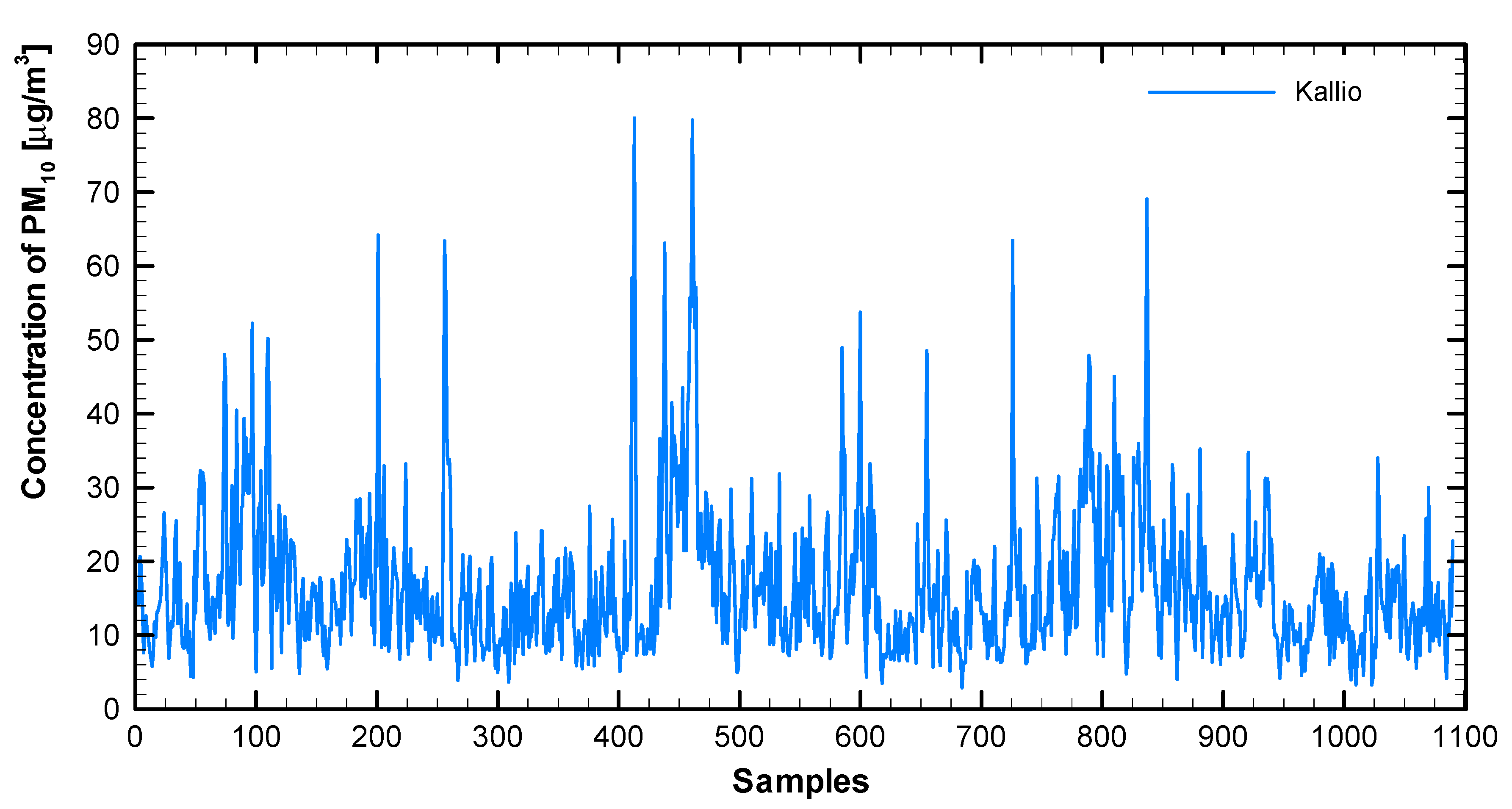
| Kallio–PM10 | 1090 | Jan 1st 2001 to Dec 31st 2003 | [66] |
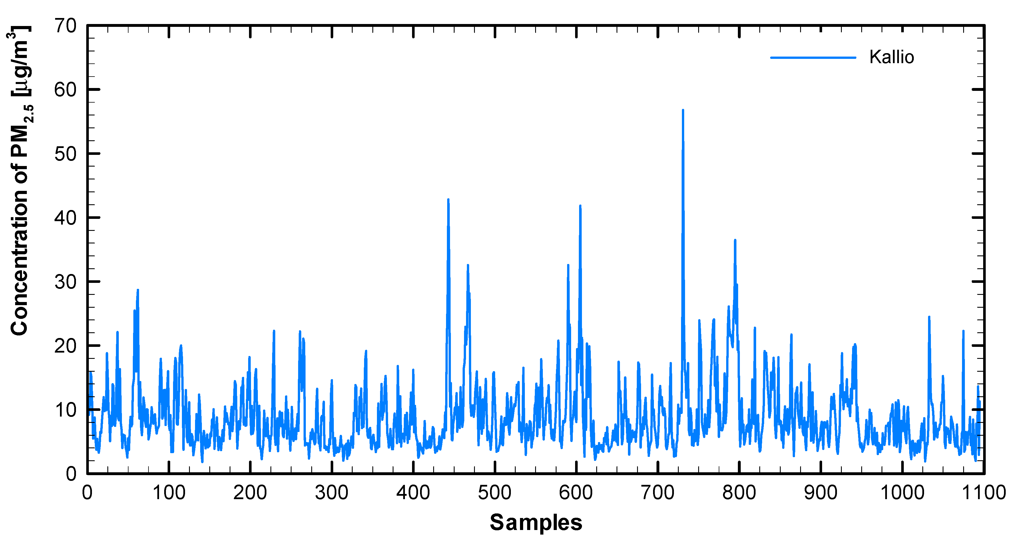
| Kallio–PM2.5 | 1095 | Jan 1st 2001 to Dec 31st 2003 | [66] |
| Vallila–PM10 | 1092 | Jan 1st 2001 to Dec 31st 2003 | [66] |
| São Paulo–PM10 | 1095 | Jan 1st 2017 to Dec 31st 2019 | [67] |
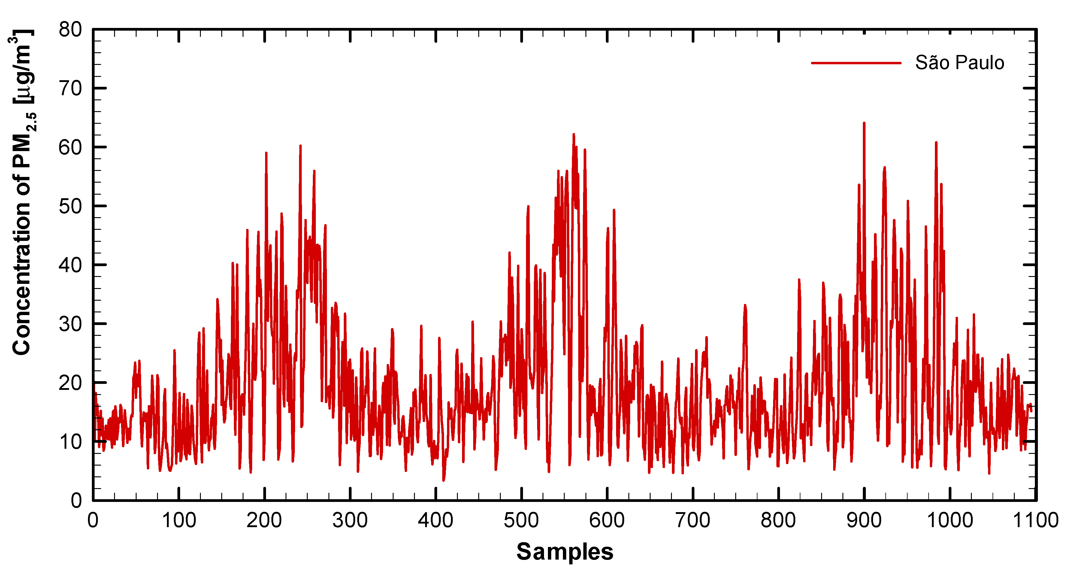
| São Paulo–PM2.5 | 1095 | Jan 1st 2017 to Dec 31st 2019 | [67] |
| Campinas–PM10 | 731 | Jan 1st 2007 to Dec 31st 2008 | [67] |
| Ipojuca–PM10 | 632 | Jul 17th 2015 to Apr 9th 2017 | [68] |
| Pollutant | Station | Mean | S. Deviation | Max | Min |
|---|---|---|---|---|---|
| PM10 [µg/m3] | Kallio | 16.7 | 9.91 | 80.0 | 2.9 |
| Vallila | 20.3 | 12.69 | 138.0 | 3.1 | |
| São Paulo | 32.1 | 17.30 | 102.4 | 5.5 | |
| Campinas | 38.0 | 15.25 | 128.7 | 12.2 | |
| Ipojuca | 35.8 | 11.13 | 78.7 | 2.8 | |
| PM2.5 [µg/m3] | Kallio | 8.8 | 5.48 | 56.8 | 1.8 |
| São Paulo | 19.7 | 11.37 | 64.1 | 3.4 |
| Partition | Coefficient of Variation (CV) | Mean CV | ||||||||||||
|---|---|---|---|---|---|---|---|---|---|---|---|---|---|---|
| Kallio PM10 | Without Partition (whole series) | 0.60 | 0.60 | |||||||||||
| Annual Partition | 0.55 | 0.68 | 0.54 | 0.59 | ||||||||||
| Monthly Partition | 0.44 | 0.69 | 0.49 | 0.53 | 0.40 | 0.36 | 0.48 | 0.57 | 0.68 | 0.56 | 0.39 | 0.54 | 0.51 | |
| Kallio PM2.5 | Without Partition (whole series) | 0.62 | 0.62 | |||||||||||
| Annual Partition | 0.54 | 0.69 | 0.60 | 0.61 | ||||||||||
| Monthly Partition | 0.52 | 0.64 | 0.71 | 0.48 | 0.48 | 0.37 | 0.39 | 0.74 | 0.60 | 0.57 | 0.48 | 0.80 | 0.57 | |
| Vallila PM10 | Without Partition (whole series) | 0.63 | 0.63 | |||||||||||
| Annual Partition | 0.52 | 0.71 | 0.58 | 0.60 | ||||||||||
| Monthly Partition | 0.43 | 0.65 | 0.53 | 0.60 | 0.40 | 0.35 | 0.32 | 0.59 | 0.55 | 0.71 | 0.46 | 0.57 | 0.51 | |
| S Paulo PM10 | Without Partition (whole series) | 0.52 | 0.52 | |||||||||||
| Annual Partition | 0.54 | 0.56 | 0.51 | 0.53 | ||||||||||
| Monthly Partition | 0.33 | 0.4 | 0.37 | 0.45 | 0.46 | 0.44 | 0.46 | 0.59 | 0.50 | 0.42 | 0.36 | 0.37 | 0.43 | |
| S Paulo PM2.5 | Without Partition (whole series) | 0.57 | 0.57 | |||||||||||
| Annual Partition | 0.56 | 0.60 | 0.56 | 0.57 | ||||||||||
| Monthly Partition | 0.34 | 0.38 | 0.39 | 0.45 | 0.47 | 0.48 | 0.47 | 0.59 | 0.52 | 0.42 | 0.37 | 0.35 | 0.44 | |
| Campinas PM10 | Without Partition (whole series) | 0.41 | 0.41 | |||||||||||
| Annual Partition | 0.41 | 0.37 | 0.39 | |||||||||||
| Monthly Partition | 0.28 | 0.22 | 0.30 | 0.27 | 0.35 | 0.38 | 0.35 | 0.32 | 0.44 | 0.35 | 0.24 | 0.26 | 0.31 | |
| Ipojuca PM10 | Without Partition (whole series) | 0.31 | 0.31 | |||||||||||
| Annual Partition | 0.28 | 0.32 | 0.27 | 0.29 | ||||||||||
| Monthly Partition | 0.32 | 0.31 | 0.31 | 0.24 | 0.48 | 0.24 | 0.35 | 0.30 | 0.23 | 0.21 | 0.18 | 0.22 | 0.28 | |
| Method | Jan | Feb | Mar | Apr | May | Jun | Jul | Aug | Sep | Oct | Nov | Dec |
|---|---|---|---|---|---|---|---|---|---|---|---|---|
| MLPPP | 33.79 | 54.96 | 53.72 | 27.25 | 38.33 | 10.82 | 29.72 | 7.69 | 5.20 | 54.47 | 8.24 | 15.19 |
| RBFPP | 21.41 | 35.13 | 38.06 | 24.47 | 30.08 | 9.08 | 31.14 | 4.65 | 4.73 | 34.21 | 6.83 | 15.68 |
| ELMPP | 29.42 | 79.28 | 59.10 | 31.86 | 39.42 | 15.09 | 46.66 | 14.10 | 9.09 | 42.57 | 7.58 | 20.39 |
| ESNPP | 23.59 | 56.50 | 45.52 | 32.84 | 27.31 | 8.88 | 37.14 | 7.57 | 5.24 | 36.39 | 7.48 | 16.81 |
| ARPP | 24.37 | 33.48 | 76.04 | 30.05 | 34.31 | 11.86 | 37.25 | 11.61 | 8.16 | 41.06 | 7.27 | 20.95 |
| MLPTR | 36.37 | 75.82 | 53.34 | 25.55 | 44.51 | 13.80 | 35.55 | 10.85 | 10.26 | 52.37 | 11.11 | 25.56 |
| RBFTR | 38.82 | 78.13 | 46.95 | 22.37 | 47.54 | 15.40 | 32.90 | 12.90 | 12.28 | 57.20 | 13.45 | 26.61 |
| ELMTR | 31.62 | 74.93 | 39.17 | 16.79 | 38.90 | 14.18 | 35.60 | 9.09 | 7.50 | 52.72 | 9.94 | 22.00 |
| ESNTR | 31.48 | 76.61 | 49.01 | 22.46 | 51.36 | 14.15 | 33.70 | 11.19 | 7.93 | 54.40 | 10.39 | 22.07 |
| ARTR | 103.18 | 116.57 | 173.42 | 107.56 | 113.79 | 33.00 | 51.40 | 23.00 | 20.84 | 83.75 | 32.82 | 27.27 |
| PERS | 34.87 | 57.26 | 78.32 | 32.15 | 44.92 | 16.43 | 36.32 | 15.54 | 16.74 | 72.91 | 15.24 | 32.72 |
| Method | Jan | Feb | Mar | Apr | May | Jun | Jul | Aug | Sep | Oct | Nov | Dec |
|---|---|---|---|---|---|---|---|---|---|---|---|---|
| MLPPP | 6.41 | 13.51 | 29.91 | 12.90 | 7.03 | 1.76 | 14.24 | 1.32 | 2.55 | 32.71 | 0.99 | 14.01 |
| RBFPP | 6.43 | 17.22 | 29.86 | 10.82 | 4.84 | 2.23 | 16.10 | 1.40 | 6.27 | 8.17 | 1.49 | 9.18 |
| ELMPP | 5.06 | 25.50 | 27.43 | 18.22 | 6.95 | 3.63 | 12.08 | 3.41 | 7.69 | 33.36 | 1.94 | 16.64 |
| ESNPP | 8.45 | 15.02 | 24.61 | 11.34 | 6.75 | 2.20 | 4.82 | 2.99 | 5.50 | 28.27 | 1.95 | 12.93 |
| ARPP | 11.39 | 16.73 | 56.51 | 22.50 | 7.17 | 2.73 | 11.29 | 2.16 | 7.28 | 30.48 | 1.85 | 14.34 |
| MLPTR | 9.35 | 36.07 | 43.18 | 20.21 | 7.58 | 4.09 | 20.30 | 2.58 | 9.59 | 37.35 | 2.12 | 20.92 |
| RBFTR | 39.13 | 46.18 | 46.49 | 52.77 | 20.02 | 6.78 | 22.89 | 3.73 | 26.26 | 31.27 | 10.69 | 36.23 |
| ELMTR | 4.95 | 31.75 | 42.73 | 17.92 | 7.33 | 3.56 | 12.72 | 2.23 | 8.06 | 34.14 | 2.15 | 18.79 |
| ESNTR | 11.86 | 25.83 | 40.35 | 21.53 | 7.98 | 4.15 | 11.88 | 3.51 | 9.16 | 35.85 | 1.84 | 21.25 |
| ARTR | 58.30 | 188.61 | 217.16 | 92.71 | 30.99 | 17.01 | 79.73 | 7.10 | 60.99 | 106.93 | 10.98 | 34.32 |
| PERS | 16.40 | 22.77 | 67.26 | 29.09 | 9.08 | 4.76 | 16.15 | 3.02 | 14.46 | 44.13 | 2.47 | 33.33 |
| Method | Jan | Feb | Mar | Apr | May | Jun | Jul | Aug | Sep | Oct | Nov | Dec |
|---|---|---|---|---|---|---|---|---|---|---|---|---|
| MLPPP | 42.06 | 76.13 | 75.64 | 30.58 | 27.42 | 23.16 | 17.79 | 6.40 | 74.74 | 73.58 | 16.43 | 22.69 |
| RBFPP | 18.75 | 59.08 | 80.90 | 45.65 | 22.84 | 23.91 | 14.08 | 4.33 | 37.84 | 35.48 | 12.67 | 17.96 |
| ELMPP | 47.77 | 86.75 | 180.87 | 68.37 | 20.55 | 25.88 | 21.18 | 11.39 | 75.77 | 75.67 | 7.85 | 27.25 |
| ESNPP | 34.15 | 31.77 | 176.27 | 83.43 | 25.28 | 13.41 | 9.92 | 7.13 | 59.59 | 34.95 | 14.92 | 17.91 |
| ARPP | 48.33 | 74.74 | 199.81 | 58.92 | 31.84 | 44.52 | 10.63 | 8.01 | 84.54 | 84.54 | 15.19 | 26.91 |
| MLPTR | 60.01 | 107.66 | 260.43 | 38.51 | 34.04 | 40.02 | 26.00 | 7.54 | 75.85 | 75.85 | 9.72 | 21.69 |
| RBFTR | 58.16 | 84.31 | 242.66 | 59.80 | 23.17 | 56.10 | 30.12 | 8.30 | 90.22 | 90.22 | 12.79 | 21.92 |
| ELMTR | 59.38 | 102.80 | 228.67 | 42.17 | 36.35 | 36.13 | 24.36 | 8.16 | 84.25 | 84.25 | 9.53 | 22.17 |
| ESNTR | 71.34 | 115.27 | 239.23 | 50.10 | 44.84 | 49.51 | 25.52 | 8.67 | 98.79 | 98.79 | 11.26 | 20.20 |
| ARTR | 340.26 | 390.36 | 1562.82 | 223.77 | 170.67 | 176.45 | 126.24 | 29.43 | 158.63 | 158.63 | 36.32 | 43.24 |
| PERS | 73.55 | 105.38 | 332.57 | 56.22 | 46.08 | 58.54 | 23.38 | 10.83 | 135.86 | 135.86 | 13.34 | 29.02 |
| Method | Jan | Feb | Mar | Apr | May | Jun | Jul | Aug | Sep | Oct | Nov | Dec |
|---|---|---|---|---|---|---|---|---|---|---|---|---|
| MLPPP | 83.18 | 25.43 | 35.11 | 40.66 | 88.37 | 86.17 | 96.45 | 75.08 | 226.37 | 19.76 | 55.82 | 18.78 |
| RBFPP | 99.12 | 7.27 | 34.05 | 43.42 | 78.31 | 98.97 | 39.80 | 61.14 | 370.70 | 25.03 | 38.71 | 9.96 |
| ELMPP | 88.20 | 16.73 | 34.62 | 62.27 | 107.28 | 93.21 | 101.08 | 135.57 | 241.65 | 27.67 | 51.69 | 16.74 |
| ESNPP | 73.61 | 9.31 | 21.02 | 68.25 | 87.18 | 96.13 | 71.79 | 39.88 | 260.88 | 48.37 | 35.96 | 15.69 |
| ARPP | 75.76 | 13.27 | 25.09 | 81.89 | 95.36 | 131.43 | 126.04 | 103.74 | 304.84 | 46.40 | 39.04 | 17.09 |
| MLPTR | 115.94 | 27.97 | 31.68 | 139.21 | 125.65 | 136.33 | 231.53 | 170.03 | 284.37 | 120.30 | 100.27 | 17.80 |
| RBFTR | 133.41 | 26.47 | 70.20 | 119.44 | 192.56 | 225.62 | 256.58 | 180.61 | 316.18 | 98.14 | 103.74 | 16.50 |
| ELMTR | 124.15 | 28.85 | 32.10 | 135.68 | 118.77 | 125.79 | 207.64 | 151.44 | 266.64 | 110.73 | 92.64 | 14.38 |
| ESNTR | 102.98 | 13.89 | 28.01 | 136.71 | 150.38 | 171.41 | 220.79 | 172.95 | 270.97 | 74.31 | 103.01 | 15.37 |
| ARTR | 138.64 | 52.17 | 55.57 | 191.96 | 221.42 | 306.05 | 496.17 | 408.73 | 562.43 | 189.19 | 174.39 | 26.71 |
| PERS | 131.44 | 32.44 | 60.26 | 148.14 | 215.47 | 183.56 | 231.51 | 127.88 | 435.96 | 138.17 | 119.08 | 21.86 |
| Method | Jan | Feb | Mar | Apr | May | Jun | Jul | Aug | Sep | Oct | Nov | Dec |
|---|---|---|---|---|---|---|---|---|---|---|---|---|
| MLPPP | 10.30 | 2.75 | 7.99 | 2.46 | 43.76 | 36.35 | 49.64 | 49.46 | 65.77 | 20.48 | 10.34 | 6.13 |
| RBFPP | 27.55 | 3.16 | 10.34 | 8.82 | 34.71 | 21.27 | 46.34 | 47.50 | 96.53 | 13.56 | 17.09 | 4.80 |
| ELMPP | 15.71 | 4.26 | 9.18 | 20.40 | 59.60 | 53.02 | 40.52 | 54.93 | 36.99 | 21.25 | 18.95 | 6.26 |
| ESNPP | 26.91 | 2.58 | 10.56 | 18.69 | 30.11 | 36.65 | 34.22 | 39.47 | 67.48 | 16.16 | 15.20 | 7.35 |
| ARPP | 26.65 | 2.82 | 12.17 | 18.55 | 45.33 | 52.59 | 58.11 | 61.25 | 100.75 | 19.41 | 16.53 | 6.99 |
| MLPTR | 39.48 | 5.36 | 14.21 | 38.17 | 61.94 | 70.72 | 131.36 | 78.94 | 108.48 | 30.30 | 40.51 | 10.96 |
| RBFTR | 39.14 | 6.52 | 19.48 | 31.39 | 83.84 | 55.69 | 107.52 | 67.57 | 100.25 | 38.46 | 46.33 | 9.52 |
| ELMTR | 33.93 | 5.48 | 13.55 | 39.54 | 45.88 | 54.51 | 109.71 | 64.24 | 104.51 | 33.89 | 40.00 | 10.29 |
| ESNTR | 27.69 | 5.54 | 13.17 | 40.31 | 59.88 | 90.64 | 116.58 | 76.05 | 95.36 | 35.81 | 41.80 | 11.45 |
| ARTR | 33.36 | 6.75 | 19.42 | 58.86 | 89.82 | 97.71 | 291.64 | 153.85 | 241.77 | 74.66 | 79.37 | 16.97 |
| PERS | 30.93 | 8.21 | 22.38 | 42.97 | 100.33 | 79.20 | 127.24 | 75.87 | 146.63 | 48.68 | 56.56 | 11.55 |
| Method | Jan | Feb | Mar | Apr | May | Jun | Jul | Aug | Sep | Oct | Nov | Dec |
|---|---|---|---|---|---|---|---|---|---|---|---|---|
| MLPPP | 14.87 | 11.50 | 64.03 | 33.67 | 91.46 | 59.00 | 76.03 | 302.27 | 42.71 | 37.54 | 32.52 | 43.23 |
| RBFPP | 7.84 | 9.42 | 31.84 | 28.78 | 104.30 | 74.89 | 44.87 | 276.74 | 94.13 | 33.39 | 32.20 | 67.83 |
| ELMPP | 10.61 | 9.48 | 47.14 | 36.83 | 88.62 | 97.08 | 43.59 | 359.92 | 38.84 | 59.05 | 29.68 | 47.04 |
| ESNPP | 16.19 | 14.89 | 43.80 | 20.99 | 46.39 | 107.17 | 38.97 | 238.39 | 39.71 | 40.45 | 17.74 | 36.03 |
| ARPP | 14.82 | 12.04 | 79.41 | 21.58 | 71.48 | 118.86 | 56.20 | 384.12 | 79.95 | 60.59 | 27.02 | 45.84 |
| MLPTR | 12.00 | 12.01 | 75.01 | 36.68 | 122.75 | 91.17 | 56.64 | 354.30 | 51.96 | 72.35 | 26.60 | 39.30 |
| RBFTR | 13.47 | 16.47 | 94.06 | 48.51 | 265.75 | 71.91 | 68.07 | 320.24 | 63.64 | 82.74 | 28.48 | 41.46 |
| ELMTR | 13.85 | 13.33 | 75.25 | 36.34 | 105.96 | 80.75 | 51.02 | 212.47 | 48.42 | 63.18 | 27.62 | 38.44 |
| ESNTR | 8.75 | 17.38 | 57.54 | 35.75 | 78.01 | 49.80 | 52.17 | 380.44 | 39.54 | 63.29 | 21.21 | 48.57 |
| ARTR | 47.70 | 30.00 | 200.80 | 188.40 | 340.38 | 219.91 | 127.13 | 993.01 | 119.35 | 269.66 | 85.60 | 103.41 |
| PERS | 14.13 | 20.62 | 116.89 | 42.52 | 96.52 | 85.77 | 76.56 | 578.28 | 74.19 | 105.49 | 40.91 | 60.30 |
| Method | Jan | Feb | Mar | Apr | May | Jun | Jul | Aug | Sep | Oct | Nov | Dec |
|---|---|---|---|---|---|---|---|---|---|---|---|---|
| MLPPP | 41.26 | 81.25 | 19.32 | 20.55 | 176.04 | 72.43 | 53.04 | 21.50 | 19.38 | 43.25 | 20.11 | 6.56 |
| RBFPP | 97.72 | 38.99 | 22.46 | 21.20 | 137.01 | 62.80 | 33.18 | 79.39 | 9.88 | 53.88 | 31.14 | 11.34 |
| ELMPP | 102.74 | 33.55 | 33.03 | 24.10 | 176.59 | 58.18 | 34.86 | 49.75 | 21.46 | 44.68 | 11.47 | 8.12 |
| ESNPP | 23.09 | 16.03 | 26.33 | 16.35 | 108.81 | 46.49 | 40.17 | 73.25 | 11.57 | 30.73 | 19.35 | 7.63 |
| ARPP | 21.98 | 20.80 | 26.80 | 15.74 | 87.27 | 48.01 | 45.54 | 127.38 | 20.42 | 52.57 | 23.03 | 3.80 |
| MLPTR | 34.84 | 44.61 | 38.83 | 15.46 | 147.92 | 100.06 | 57.74 | 89.10 | 13.78 | 72.92 | 14.47 | 8.24 |
| RBFTR | 31.00 | 147.25 | 37.94 | 19.70 | 126.84 | 89.11 | 63.83 | 173.77 | 11.00 | 75.68 | 15.58 | 11.54 |
| ELMTR | 33.24 | 61.78 | 32.99 | 14.70 | 126.62 | 104.05 | 59.12 | 41.04 | 15.78 | 78.06 | 13.62 | 8.44 |
| ESNTR | 23.10 | 43.11 | 31.63 | 9.11 | 121.14 | 86.48 | 39.17 | 135.14 | 17.35 | 62.38 | 13.20 | 8.51 |
| ARTR | 45.91 | 46.49 | 79.73 | 61.37 | 563.32 | 238.31 | 102.43 | 248.19 | 34.55 | 99.80 | 29.17 | 21.24 |
| PERS | 37.05 | 49.25 | 46.55 | 19.90 | 227.81 | 141.80 | 66.80 | 213.59 | 18.60 | 84.85 | 16.96 | 16.98 |
| Jan | Feb | Mar | Apr | May | Jun | Jul | Aug | Sep | Oct | Nov | Dec | Total | |
|---|---|---|---|---|---|---|---|---|---|---|---|---|---|
| MLPPP | 1 | 1 | 3 | 3 | - | 1 | 1 | 2 | 2 | 1 | 2 | 1 | 18 |
| RBFPP | 3 | 2 | 2 | 1 | 2 | 1 | 2 | 2 | 3 | 3 | 2 | 4 | 27 |
| ELMPP | - | - | - | - | 1 | - | - | - | 2 | - | 2 | - | 5 |
| ESNPP | 1 | 3 | 2 | 1 | 3 | 4 | 4 | 2 | - | 3 | 1 | 1 | 25 |
| ARPP | 1 | 1 | - | - | 1 | - | - | - | - | - | - | 1 | 4 |
| MLPTR | - | - | - | - | - | - | - | - | - | - | - | - | - |
| RBFTR | - | - | - | - | - | - | - | - | - | - | - | - | - |
| ELMTR | 1 | - | - | 1 | - | - | - | 1 | - | - | - | - | 3 |
| ESNTR | - | - | - | 1 | - | 1 | - | - | - | - | - | - | 2 |
| ARTR | - | - | - | - | - | - | - | - | - | - | - | - | - |
| PERS | - | - | - | - | - | - | - | - | - | - | - | - | - |
© 2020 by the authors. Licensee MDPI, Basel, Switzerland. This article is an open access article distributed under the terms and conditions of the Creative Commons Attribution (CC BY) license (http://creativecommons.org/licenses/by/4.0/).
Share and Cite
de Mattos Neto, P.S.G.; Marinho, M.H.N.; Siqueira, H.; de Souza Tadano, Y.; Machado, V.; Antonini Alves, T.; de Oliveira, J.F.L.; Madeiro, F. A Methodology to Increase the Accuracy of Particulate Matter Predictors Based on Time Decomposition. Sustainability 2020, 12, 7310. https://doi.org/10.3390/su12187310
de Mattos Neto PSG, Marinho MHN, Siqueira H, de Souza Tadano Y, Machado V, Antonini Alves T, de Oliveira JFL, Madeiro F. A Methodology to Increase the Accuracy of Particulate Matter Predictors Based on Time Decomposition. Sustainability. 2020; 12(18):7310. https://doi.org/10.3390/su12187310
Chicago/Turabian Stylede Mattos Neto, Paulo S. G., Manoel H. N. Marinho, Hugo Siqueira, Yara de Souza Tadano, Vivian Machado, Thiago Antonini Alves, João Fausto L. de Oliveira, and Francisco Madeiro. 2020. "A Methodology to Increase the Accuracy of Particulate Matter Predictors Based on Time Decomposition" Sustainability 12, no. 18: 7310. https://doi.org/10.3390/su12187310
APA Stylede Mattos Neto, P. S. G., Marinho, M. H. N., Siqueira, H., de Souza Tadano, Y., Machado, V., Antonini Alves, T., de Oliveira, J. F. L., & Madeiro, F. (2020). A Methodology to Increase the Accuracy of Particulate Matter Predictors Based on Time Decomposition. Sustainability, 12(18), 7310. https://doi.org/10.3390/su12187310