Using Remote Sensing Data to Study the Coupling Relationship between Urbanization and Eco-Environment Change: A Case Study in the Guangdong-Hong Kong-Macao Greater Bay Area

Abstract

Promoting the coordinated development of urbanization and eco-environment is essential for the development of urban agglomerations. As an emerging economic growth pole in China, the Guangdong-Hong Kong-Macao Greater Bay Area (GBA) has become a research hotspot in recent years. However, relevant studies in this area have been largely constrained by the incomparability of statistical data between the inland part of the GBA and the two Special Administrative Regions (Hong Kong and Macao) of the GBA. This study used nighttime light data and the normalized difference vegetation index (NDVI) to evaluate the level of urbanization and eco-environment in the GBA, respectively. Then we adopted the gravity center model to analyze the overall coupling situation between urbanization and eco-environment change. We also adopted a coordination index to determine the spatial differentiation characteristics of this coupling in the GBA from 2000 to 2018. The results show that (1) the spatial pattern of urbanization and eco-environment both show an approximately circular structure, and the change rates of these two variables show significant spatiotemporal differentiation; (2) on the whole, urban development and eco-environment construction became more coupled in the GBA during 2000–2018, as indicated by the continuously decreasing distance between the gravity centers of urbanization and eco-environment; and (3) as for the spatial differentiation characteristic of this coupling, the GBA was generally dominated by slightly uncoupled units, while the spatial distribution of different coupling types transformed from a circular structure to a relatively random form.

1. Introduction

In the past few decades, China has experienced unprecedented urbanization and economic development. According to a blue paper report released by Morgan Stanley in 2019, titled “The Rise of China’s Supercities: New Era of Urbanization” [1], the country’s urbanization rate will reach 75% by 2030, driven by city clusters, smart cities, and agricultural modernization (the growth of China’s agricultural labor productivity over the next decade is expected to free up more rural population for further urbanization). This new era of urbanization (which is referred to as “Urbanization 2.0”) is expected to increase China’s urban population by 220 million by 2030, half of which are predicted to settle in China’s five largest city clusters, namely the Yangtze River Delta, the Jing-Jin-Ji Area, the Guangdong-Hong Kong-Macao Greater Bay Area, the Mid-Yangtze River Area, and the Chengdu-Chongqing Area. However, population aggregation in big cities is always accompanied by rising levels of environmental pollution, which poses the main threat to the sustainable development of urbanization and eco-environment.

The concept of coupling is derived from physics and refers to the phenomenon that two or more systems influence each other through various kinds of interactions [2]. Previous studies have shown that there is an objective interactive coupling relationship between urbanization and eco-environment [3,4]. This complex system, which is often called “the interactive coupling system of urbanization and ecological environment”, can be regarded as an on-limits and non-equilibrium dynamic fluctuating system with non-linear interaction and self-organization capability [5]. Fang et al. [6] proposed six major laws of this system, namely the coupling fission law, dynamic hierarchy law, stochastic fluctuations law, non-linear synergetic law, threshold value law, and forewarning law, which have important theoretical guiding significance to reveal the interactive coercing relationship and dynamic coupling relationship between urbanization and eco-environment. Different evaluation indices or models for coupling analyses have been proposed in studies of urbanization and eco-environment. These indices and models are also widely applied in relevant research. For example, Hu et al. [7] proposed a coordination index and conducted a quantitative analysis of the coordination of the three aspects of urbanization (the population urbanization, the land urbanization, and the economic urbanization), and Zhang et al. [8] used this index to conduct relevance analysis of the evolution of population urbanization and industrial urbanization in Qinghai Province, China. Fan et al. [9] proposed the gravity center model to determine the coupling process between economy and population by measuring the overlapping between the two gravity centers and the consistency of their movement tracks, and Yang et al. [10] employed this model to study the coupling relationship between construction land expansion and urban heat-island expansion in the Guangdong-Hong Kong-Macao Greater Bay Area (GBA).

The GBA is the fourth-largest bay area in the world after the New York Bay Area, the San Francisco Bay Area, and the Tokyo Bay Area. In recent decades, the development of the GBA has gone through an isolation stage (before 1978), a diffusion stage (1979–2014), and a symbiotic stage (after 2015) [11,12,13]. Since 1 July 2017, the GBA has officially been incorporated into China’s national strategies, which was marked by the signature of the “Framework Agreement on Deepening Guangdong-Hong Kong-Macao Cooperation in the Development of the Bay Area” in Hong Kong. It is planned to build the GBA into a world-class urban agglomeration in the form of “9 + 2”, namely nine cities in the Pearl River Delta and two Special Administrative Regions, which is expected to be an important driving force for global economic development and technological innovation. However, most studies of the GBA mainly focused on its function orientation [14,15], intra- and inter-regional relationships [16,17], and development strategies [18,19] but paid little attention to the coordinated development of its urbanization and eco-environment.

This lack of research may be partly due to the incomparability of statistics between the inland part of the GBA and the Hong Kong-Macao area. The main incomparability issue is that the economic statistics (e.g., economic growth factors and economic cycle) from the inland part of the GBA is not applicable to the Hong Kong-Macao area. Fortunately, the availability of multi-temporal remote sensing data with increasing spatial resolution and coverage has enabled more accurate and extensive monitoring of changes in urbanization and eco-environment, which allows the analysis of the social-economic-natural compound ecosystem across administrative boundaries. Nighttime light (NTL) data, including DMSP/OLS (Defense Meteorological Satellite Program Operational Linescan System, Department of Defense, USDOD, Arlington, VA, USA) data and NPP/VIIRS (National Polar-orbiting Partnership satellite’s Visible Infrared Imaging Radiometer Suite, Raytheon Technologies, Waltham, MA, USA) data, is one of the most common data types in such studies. NTL data has been widely used in studies of urban expansion [20,21,22], economic activity evaluation [23,24,25], population estimation [26,27,28,29], energy consumption and carbon emissions [30,31,32,33,34], light pollution [35], and disaster assessment [36], etc. Due to the discontinuity in the time series of DMSP/OLS data and NPP/VIIRS data, the combination of the two data types increases the utility of NTL data in these studies. Li et al. [37] proposed a method for integrating DMSP/OLS and NPP/VIIRS data to evaluate the city light dynamics in Syria during the civil war (2011–present), which effectively extended the temporal coverage of NTL data.

The normalized difference vegetation index (NDVI) is another widely used type of remote sensing data in the study of socio-economic activities and environmental change. It reflects the vegetation growth state and vegetation coverage, which can be used to effectively detect spatiotemporal patterns of above-ground vegetation dynamics [38,39]. In particular, the annual variation of the NDVI has been extensively used to assess the impacts of human activities on the urban eco-environment [40].

With the incorporation of GBA into China’s national strategies, this region has been recognized as a hotspot for future research. This study used NTL data and the NDVI to solve the problem of the incomparability of statistics between the inland part of the GBA and the Hong Kong-Macao area. The mean nighttime light (MNL) and the yearly maximum value of the NDVI were used to represent the level of urbanization and the level of eco-environment, respectively. Then, we adopted the gravity center model to analyze the overall coupling situation between urbanization and eco-environment and the coordination index to analyze the spatial differentiation characteristics of this coupling. This study was intended to (1) reveal the spatiotemporal patterns of urbanization and eco-environment in the GBA; (2) identify the overall coupling situation between urbanization and eco-environment change in the GBA; and (3) analyze the spatial differentiation characteristics of this coupling during different periods in the GBA. The results of this study are of important guiding significance to promote the coordinated development of urbanization and eco-environment in the GBA. Figure 1 is a flowchart showing the methodology of this study.

2. Study Area and Data

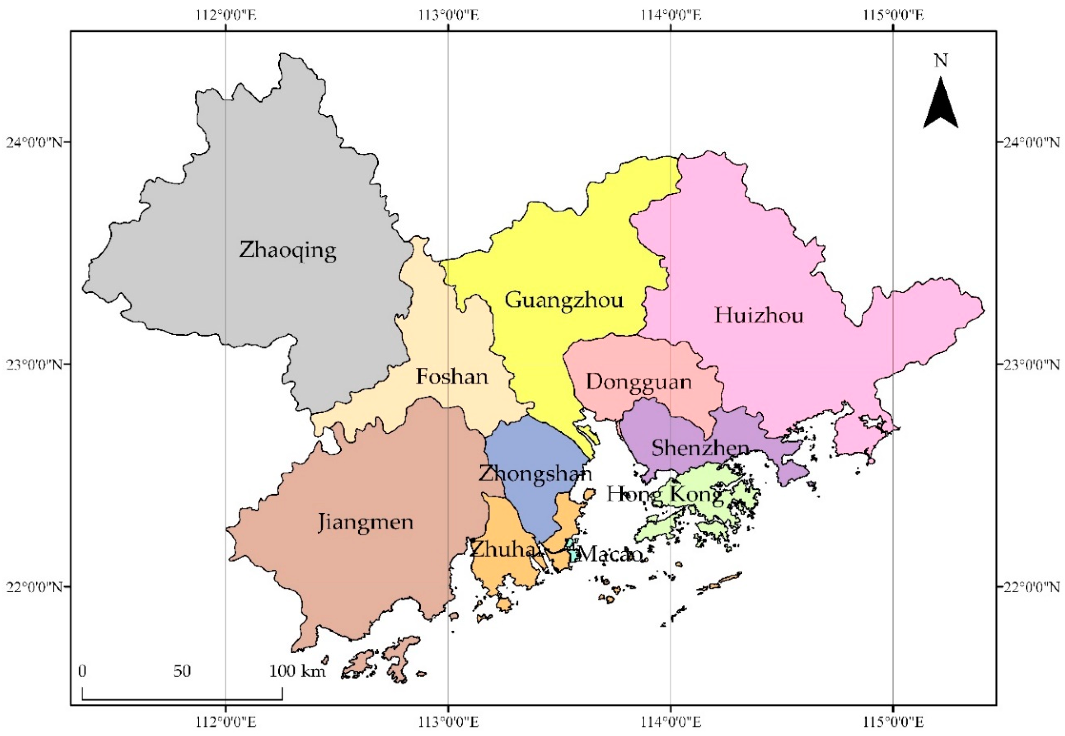
2.1. Study Area

The GBA is located at 111°12′–115°35′ E and 21°25′–24°30′ N and consists of nine cities in Guangdong Province (Guangzhou, Shenzhen, Foshan, Dongguan, Zhongshan, Zhuhai, Huizhou, Jiangmen, and Zhaoqing) and two Special Administrative Regions (Hong Kong and Macao) (Figure 2). Its total area is 56,000 km², and its population had reached 71.51 million by the end of 2018 [41].

As one of the most urbanized city agglomerations in the world, this region is expected to promote the cooperative development of the Pan-Pearl River Delta and construct a new open economic system for further integration into the world economy [16]. Up to now, two core areas—the Guangzhou-Foshan core area and the Hong Kong-Shenzhen core area, have emerged in the GBA, which will become new potential growth poles in the regional integration of the GBA. On the other hand, the boundary effect has reduced remarkably and border areas are growing rapidly in the GBA [42], especially the border regions of Shenzhen-Dongguan, Shenzhen-Huizhou, Dongguan-Huizhou, Guangzhou-Dongguan, and Guangzhou-Foshan. Under this development trend, the GBA will play a crucial role in the implementation of the national regional development strategy and the sustainable development of Hong Kong and Macao.

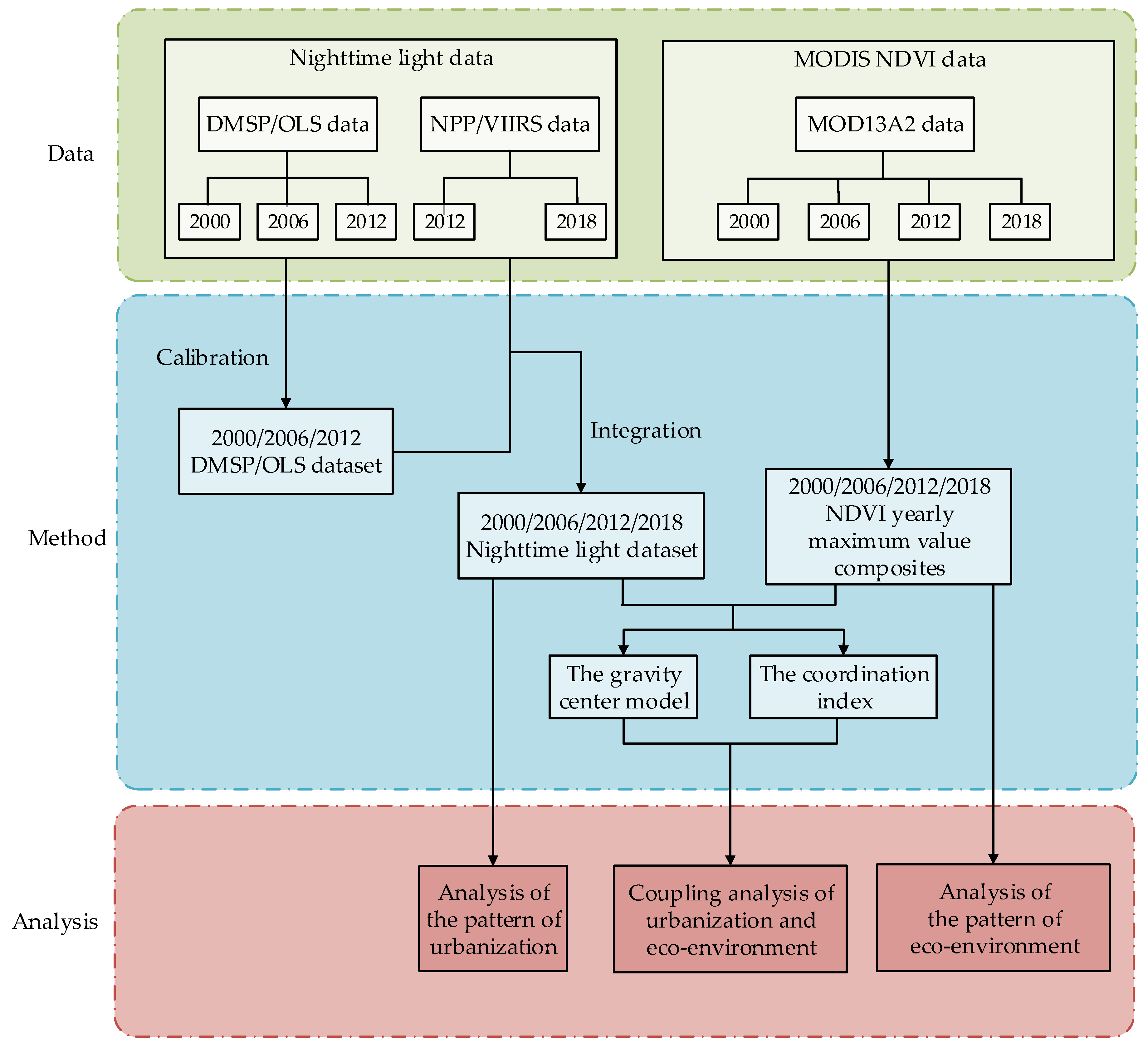
2.2. Data Sources and Pre-Processing

The data used in this study included remote sensing data and administrative border data. The remote sensing data included NTL data and MODIS (Moderate-Resolution Imaging Spectroradiometer) NDVI data. The administrative border data included the boundary of the GBA and the boundaries of the 620 township (street) units in the GBA. Both the NTL data and NDVI data were extracted according to the boundary of the GBA.

2.2.1. Nighttime Light Data

DMSP/OLS data are provided in 30-arc-second grids, with only one band containing a greyscale value. The visible band has 6-bit quantization, producing a digital number (DN) value ranging from 0 to 63 for each pixel [43]. These data can be used to detect artificial lights, such as those from human settlements, fires, gas flares, and fishing boats, as well as lightning and the aurora [36,44]. Currently, the products of DMSP/OLS include three kinds of annual average data: average visible, stable lights, and cloud-free coverage. The night stable light is an annual cloud-free composite of the average DN value for the detected lights (e.g., lights from cities, towns, and other sites with persistent lighting) with ephemeral lights and background noise removed [45]. Therefore, we chose stable light data in our study. The data were not available subsequent to February 2014 [37]. In 2011, NASA (National Aeronautics and Space Administration, Washington, DC, USA) and NOAA (National Oceanic and Atmospheric Administration, Silver Spring, MD, USA) launched the Suomi National Polar Partnership (NPP) satellite carrying the first Visible Infrared Imaging Radiometer Suite (VIIRS) instrument. NPP/VIIRS data, which have a spatial resolution of 15 arc-seconds, include two data types: VIIRS Cloud Mask Configuration (VCMCFG) and VIIRS Cloud Mask Stray-light Corrected Configuration (VCMSLCFG). NPP/VIIRS data offer substantial improvements in spatial resolution, radiometric calibration, and usable dynamic range compared to the DMSP/OLS data [46].

This study used data from the years 2000, 2006, 2012, and 2018. We chose nighttime stable light of DMSP/OLS and VCMCFG of NPP/VIIRS in December, both of which were obtained from NGDC (National Genomics Data Center; https://ngdc.noaa.gov) (

Table 1. Data types of nighttime light data. (VCMCFG: VIIRS Cloud Mask Configuration)

Data Types	Year
	2000	2006	2012	2018
DMSP/OLS	F14 1 F15	F15 F16	F18	-
NPP/VIIRS	-	-	VCMCFG	VCMCFG

¹ F14 represents the number of the satellite. There were two satellites in 2000 and 2006. (-) no data in the specific year.

). In order to match the spatial resolution of the two datasets, the DMSP/OLS data and NPP/VIIRS data were both resampled to a pixel size of 1km and projected into the Lambert Conformal Conic projection with reference to the WGS84 coordinate system. The negative radiation values in NPP/VIIRS images were set to 0.

2.2.2. MODIS NDVI Data

A MODIS data product (MOD13A2 data) in HDF format was acquired for 2000, 2006, 2012, and 2018 from the NASA Earth Observing System (EOS) data gateway (https://ladsweb.modaps.eosdis.nasa.gov/search/). This product is provided every 16 days at a 1-km spatial resolution. The strip number of the study area is h28v06. The NDVI data were projected into the Lambert Conformal Conic projection with reference to the WGS84 coordinate system and converted to TIFF format using the Modis Reprojection Tool (MRT).

3. Methods

3.1. Evaluation Indices of Urbanization and the Eco-Environment

We chose the MNL as the evaluation index of the level of urbanization. The MNL integrates information on the built-up area and the intensity of socio-economic activities, which reflects the average intensity of human activities in the study area [47]. The MNL was calculated as follows:

$$\mathrm{MNL}=\frac{{\sum }_{i=1}^{k}D{N}_i}{k},$$

(1)

where k represents the number of pixels in the analytical unit, DN_i represents the DN value of the ith pixel. The processing of NTL data included calibration and integration, which will be further discussed in Section 3.2.

For the evaluation of the eco-environment, the yearly maximum values of the NDVI were extracted to reduce the influence of the atmosphere, aerosols, and clouds [48,49] (Figure S1). Then the mean value of the NDVI in each analytical unit was calculated to represent the level of eco-environment.

3.2. Calibration and Integration of Nighttime Light Data

3.2.1. Calibration of DMSP/OLS Data

Since DMSP/OLS sensors have no onboard radiometric calibration for the visible band [50,51], the acquired data differ from each other in terms of radiometric performance. In this section, we followed the method proposed by Cao et al. [52] to achieve radiometric and saturation calibration of the DMSP/OLS data.

Firstly, we used the power function for intercalibration (Formula (2)):

$$D{N}_{\mathrm{cal}\left(n,i\right)}=a\times D{N}_{\mathrm{orig}\left(n,i\right)}^b,$$

(2)

where DN_orig(n,i) represents the original DN value of the ith pixel of the DMSP/OLS image in the nth year, DN_cal(n,i) represents the intercalibrated DN value, and a and b are intercalibration parameters, which are listed in

Table 2. Intercalibration model parameters for each image [52].

Satellite	Year	a1	b2
F14	2000	0.9913	1.1753
F15	2000	0.8093	1.183
	2006	1.2481	1.0738
F16	2006	0.8296	1.1883
F18	2012	0.4821	1.1866

¹a represents the coefficient of the power function; ² b represents the exponent of the power function.

.

Furthermore, in order to make full use of the DMSP/OLS data derived from multiple sensors in the same year, it was necessary to perform continuity calibration using Formula (3) if there were two images in the same year.

$$\begin{gathered} D{N}_{\mathrm{con}\left(n,i\right)}=\{\begin{array}{c}0,\hspace{1em}D{N}_{\mathrm{cal}\left(n,i\right)}^1=0 \mathrm{and} D{N}_{\mathrm{cal}\left(n,i\right)}^2=0\hfill \\ \frac{D{N}_{\mathrm{cal}\left(n,i\right)}^1+D{N}_{\mathrm{cal}\left(n,i\right)}^2}{2},\mathrm{otherwise}\hfill \end{array} \\ (n=2000,2006,2012) \end{gathered}$$

(3)

where $D{N}_{\mathrm{cal}\left(n,i\right)}^1$ and $D{N}_{\mathrm{cal}\left(n,i\right)}^2$ represent the intercalibrated DN values of the two NTL images, and $D{N}_{\mathrm{con}\left(n,i\right)}$ represents the DN value after continuity calibration.

Finally, considering the accelerating urbanization process in the GBA since the start of the 21st century, further continuity calibration steps were performed using Formula (4) to ensure that the DN value of the same pixel keeps increasing over time:

$$\begin{gathered} D{N}_{\left(n,i\right)}=\{\begin{array}{c}0,D{N}_{\mathrm{con}(n+6,i)}=0\hfill \\ D{N}_{\mathrm{con}\left(n-6,i\right)},D{N}_{\mathrm{con}\left(n+6,i\right)}<0\mathrm{and}D{N}_{\text{con}\left(n-6,i\right)}<D{N}_{\mathrm{con}\left(n,i\right)}\hfill \\ D{N}_{\mathrm{con}\left(n,i\right)},\mathrm{otherwise}\hfill \end{array} \\ (n=2000,2006,2012) \end{gathered}$$

(4)

where $D{N}_{\mathrm{con}\left(n,i\right)}$ represents the DN value after the first step of continuity calibration, and $D{N}_{\left(n,i\right)}$ represents the DN value after further continuity calibration. The above calibration processes effectively solved the problem of pixel saturation in the DMSP/OLS data and greatly improved their continuity and comparability [44].

3.2.2. Integration of Nighttime Light Data

This study referred to the integration method proposed by Li et al. [37], which was used to simulate DMSP/OLS data from NPP/VIIRS data using a power function based on the temporal overlap between the two datasets. The integration process included the following three steps:

(1)

For each DN value, all pixels in the DMSP/OLS image from 2012 and the corresponding pixels in the NPP/VIIRS image for the same year were extracted. Then, the average radiation value of the extracted NPP/VIIRS pixels was calculated (Table S1, Supplementary Material), and a scatterplot was generated with the average radiation value of NPP/VIIRS data as the independent variable (the unit is nW/cm²/s) and the DN value of DMSP/OLS data as the dependent variable. We selected the pixels whose DN value was equal to or less than 50 to reduce the influence of pixel saturation [37]. The fitted curve for 2012 is shown in Figure 3. The integration function is given in Formula (5):

DN = 15.519506 × radiance^0.5510601,

(5)

where radiance represents the radiation value of the NPP/VIIRS data, and DN represents the DN value simulated from the NPP/VIIRS data.

(2)

Formula (5) was used to simulate DMSP/OLS data for 2018. Then a Gaussian low-pass filter with a window size of 3 pixels was used to smooth the simulated image.

(3)

Finally, the continuity calibration was performed again using Formula (4) to ensure the continuity of the whole dataset.

After the above calibration and integration steps, 4 nighttime light images were generated (2000, 2006, 2012, and 2018) (Figure S2). The data for 2000, 2006, and 2012 were obtained by intercalibration and continuity calibration, and the data for 2018 were obtained by simulation, filtering, and continuity calibration.

3.3. The Gravity Center Model

The gravity center model [9] was adopted to analyze the overall coupling situation of the GBA. The calculation formulas for the gravity centers of urbanization and eco-environment are shown in Formulas (6) and (7), respectively:

$$C_U\left(X,Y\right)=\frac{{\sum }_{i=1}^n\left(U_{i}C\left(x_i,y_i\right)\right)}{{\sum }_{i=1}^n{U}_i},$$

(6)

$$C_E\left(X,Y\right)=\frac{{\sum }_{i=1}^n\left(E_{i}C\left(x_i,y_i\right)\right)}{{\sum }_{i=1}^n{E}_i},$$

(7)

where C_U and C_E represent the gravity centers of urbanization and eco-environment, respectively, U_i and E_i represent the value of MNL and NDVI of the ith township (street) unit, respectively, and C(x_i, y_i) are the coordinates of the gravity center of the ith township (street) unit. The gravity center model consists of two parts: the overlapping of gravity centers and the consistency of their movement tracks.

3.3.1. Overlapping of Gravity Centers

The overlapping of gravity centers was calculated by the distance between the two gravity centers, with a shorter distance implying a higher level of coordination. The distance was calculated using Formula (8):

$$D=\sqrt{{\left(x_U-x_E\right)}^2+{\left(y_U-y_E\right)}^2},$$

(8)

where x_U (x_E) and y_U (y_E) represent the x-coordinate and y-coordinate of the gravity center of urbanization (eco-environment), respectively.

3.3.2. The Consistency of Movements

The consistency of movements was defined as the cosine of the angle (θ) between the movement tracks of the two gravity centers, which was calculated using Formula (9) according to the cosine law:

$$\begin{gathered} C=\cos \theta =\frac{\left\{\left(\Delta x_U^2+\Delta y_U^2\right)+\left(\Delta x_E^2+\Delta y_E^2\right)-\left[{\left(\Delta x_U-\Delta x_E\right)}^2+{\left(\Delta y_U-\Delta y_E\right)}^2\right]\right\}}{\left[2\sqrt{\left(\Delta x_U^2+\Delta y_U^2\right)\left(\Delta x_E^2+\Delta y_E^2\right)}\right]} \\ =\frac{\Delta x_U\Delta x_E+\Delta y_U\Delta y_E}{\sqrt{\left(\Delta x_U^2+\Delta y_U^2\right)\left(\Delta x_E^2+\Delta y_E^2\right)}}, \end{gathered}$$

(9)

where Δ x_U (Δ x_E) and Δ y_U (yx_E) represent the variations of the x-coordinate and y-coordinate of the gravity center of urbanization (eco-environment), respectively, during the specific period. The range of C was [−1,1]; C = 1 implies consistent directions of the two movement tracks, and C = −1 implies opposite directions.

3.4. The Coordination Index

Aside from the gravity center model, we adopted the coordination index [7] to evaluate the spatial differentiation characteristics of the coupling relationship between urbanization and eco-environment in the GBA. The coordination index was defined as follows:

$$C_{UE}=\frac{\left|\left(UR+ER\right)/\sqrt{2}\right|}{\sqrt{{\left(UR\right)}^2+{\left(ER\right)}^2}},$$

(10)

where C_UE represents the coordination index of urbanization and eco-environment change, and UR and ER represent the average annual change rates of the MNL and NDVI, respectively. The range of C_UE was [0,1]. When UR was equal to ER, C_UE was 1, and urbanization and eco-environment change were maximally coupled; when the absolute value of UR was equal to ER but of opposite sign, C_UE was 0, and urbanization and eco-environment change were minimally uncoupled. The classification of C_UE and the relationship between UR and ER are shown in

Table 3. Classification of the coordination index of urbanization and eco-environment change (C_UE) and the relationship between the average annual change rate of the mean nighttime light (MNL) (UR) and the average annual change rate of the normalized difference vegetation index (NDVI) (ER).

CUE	Coupling Types	Relationship between UR and ER
(0.9,1]	Superiorly coupled
(0.8,0.9]	Barely coupled	UR − ER < 0.1	UR lagged
(0.7,0.8]	Slightly uncoupled	0 ≤ |UR − ER| ≤ 0.1	coordinated
(0.5,0.7]	Moderately uncoupled	UR − ER > 0.1	ER lagged
[0,0.5]	Seriously uncoupled

(adapted from [2,7], Table S2).

4. Results and Discussion

4.1. Analysis of the Pattern of Urbanization

The MNL was calculated for each township (street) unit using Formula (1). Figure 4 shows the spatial and temporal variations of the urbanization level in the GBA. Between 2000 and 2018, the urbanization pattern mainly presented the following two characteristics.

4.1.1. A Circular Structure

On the whole, there was a large spatial differentiation of the urbanization level in the GBA (Figure 4). The high-value units were concentrated in the central area, such as the border of Guangzhou and Foshan, northern Dongguan, and most parts of Shenzhen and Hong Kong, while the low-value units were mainly distributed at the periphery, which showed a circular structure following the gradient of urbanization level. This significant imbalance was caused by several factors. Firstly, the central area is conveniently connected to other cities of the Pearl River Delta by the efficient transportation system, while the mountainous western and eastern regions are separated from central cities and mainly function as ecological barriers. Secondly, the central area has attracted a number of foreign enterprises to invest since China’s reform and opening-up and has become the first production base in the “pre-shop and post-factory” model [53]. In recent years, the industrial structure in cities in the central GBA has been continuously optimized and a high value-added modern industrial system has been gradually formed; however, peripheral cities are still in the early stages of industrialization. As a result, the gap between the center and the periphery of the GBA has further widened (Figure 4d).

4.1.2. Rise in Urban Border Areas

In recent years, the urban border areas took advantage of the cheap land and convenient transportation to undertake core industry diffusion and industrial transfer. Economic activities in the urban border areas and the cross-city cooperation between towns and streets were rather frequent [54]. As shown in Figure 4, it was found that, between 2000 and 2018, the urbanization level of border areas such as Guangzhou-Foshan, Guangzhou-Dongguan, Shenzhen-Dongguan, Shenzhen-Huizhou, and Dongguan-Huizhou significantly increased, which was closely related to the driving effects of core cities such as Guangzhou and Shenzhen.

Additionally, the change rates of the urbanization level were also found to vary greatly among different units during the three periods (Figure 5). Most units developed stably during the research period, while western Zhaoqing and eastern Huizhou developed significantly during the first and the third period, especially from 2012 to 2018. The periphery area remained underdeveloped for a long time due to its mountainous terrain (Figure S3). However, with the large-scale land development policy enacted since the start of the 21st century, most cities in the GBA, especially those in less developed regions, began to exploit their underdeveloped areas through land reclamation and expropriation (Figure 5a). By 2006, the concepts of “ecological cities” and “circular economy” were adopted in most cities in China, including those in the GBA. Therefore, urban construction entered into a relatively steady development period (Figure 5b). After 2012, Zhaoqing and Huizhou continued to exploit idle land to expand the border of the urban core area, which resulted in the rapid expansion of urban land in the peripheries of the two cities (Figure 5c).

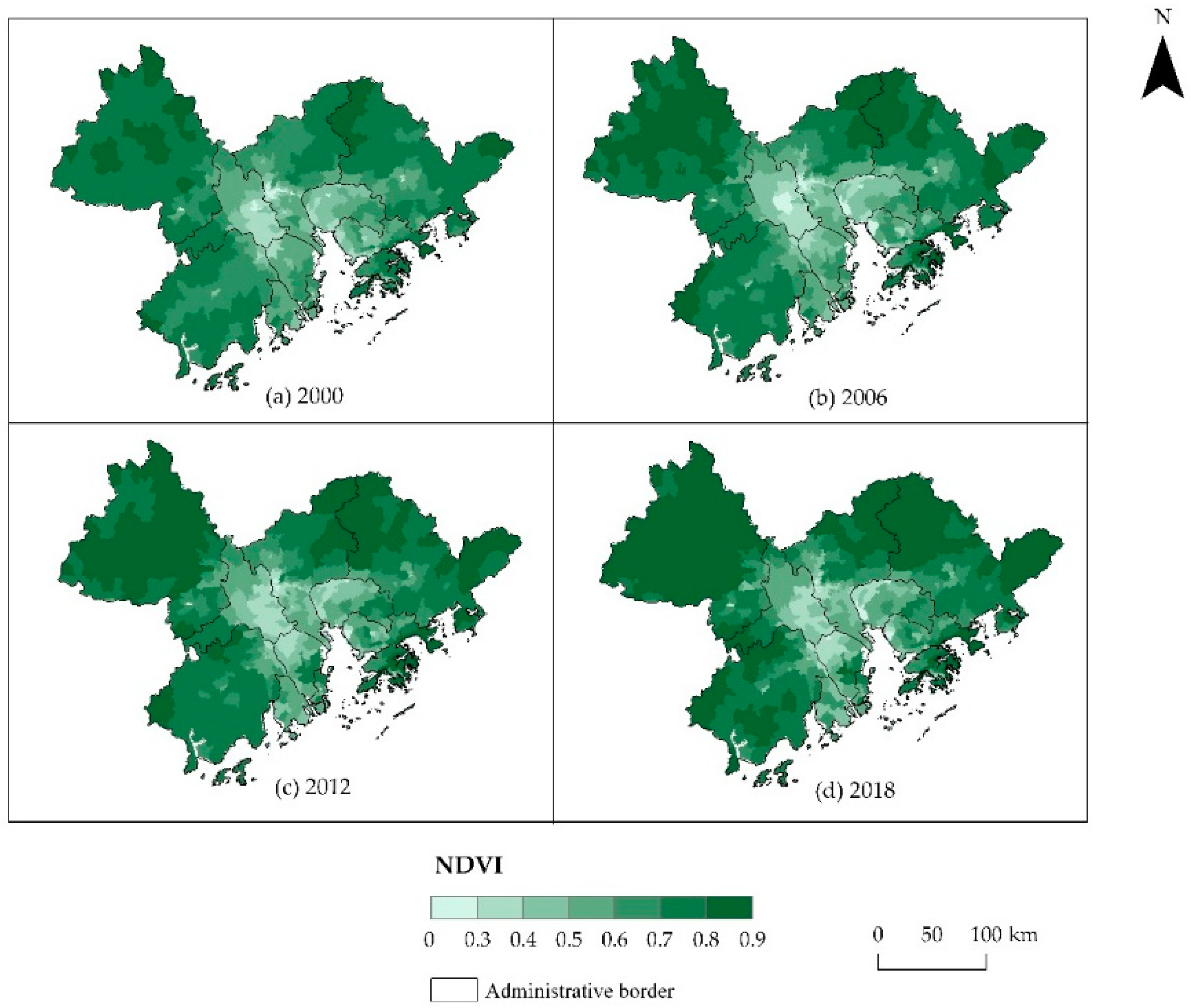
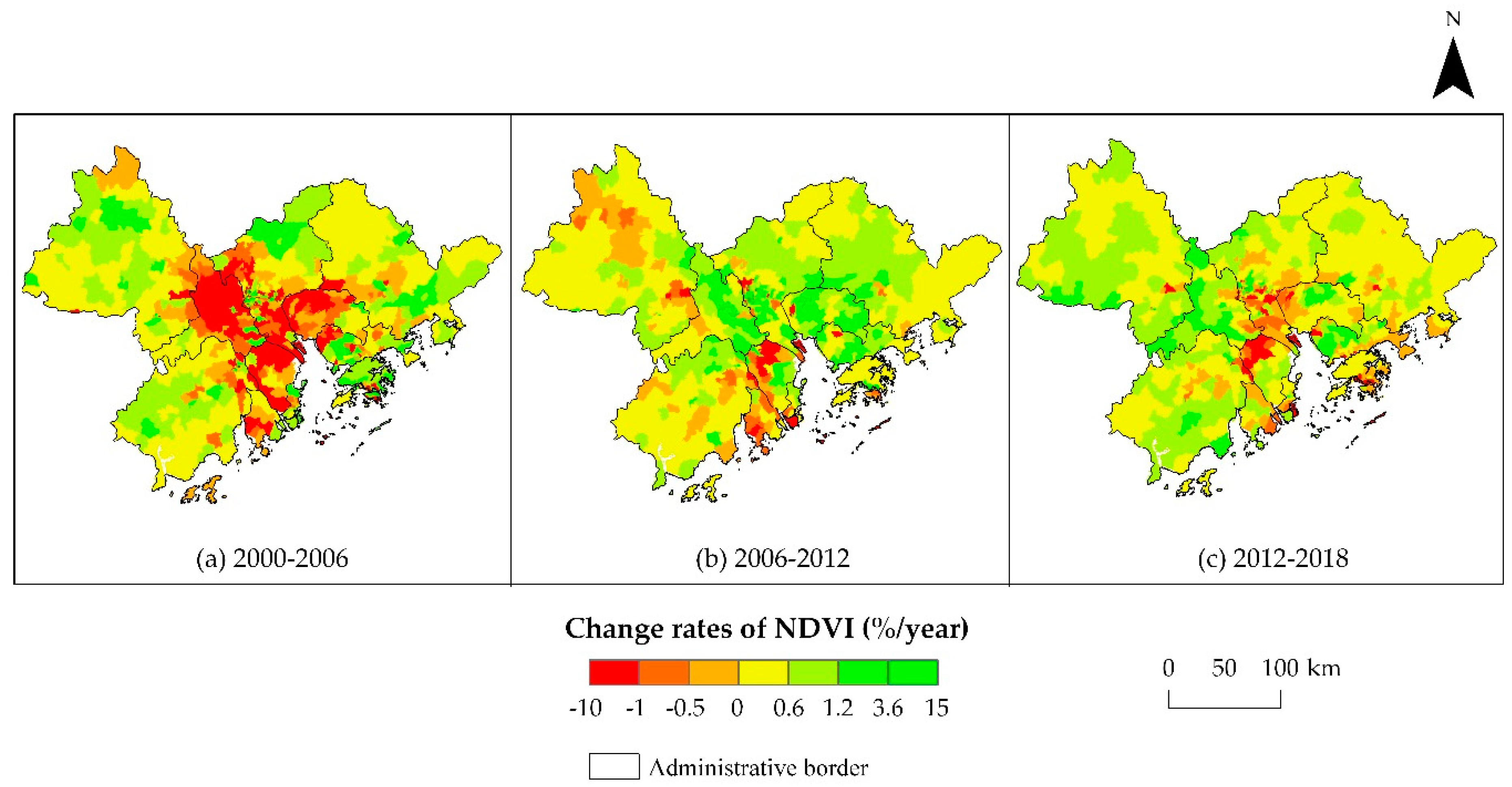
4.2. Analysis of the Pattern of Eco-Environment

The mean value of the yearly maximum value of the NDVI was calculated for each township (street) unit. Similar to the spatial pattern of urbanization (Section 4.1), the spatial pattern of the eco-environment of the township (street) units showed a circular structure (Figure 6). Areas with a high level of eco-environment were mainly concentrated in the periphery of the GBA, such as Zhaoqing, northern Huizhou, and western Jiangmen; these areas are dominated by mountains and hills and perform key ecological functions in the cities. On the contrary, in urban areas in the central GBA, the eco-environment was greatly degraded between 2000 and 2018 as a consequence of urban land exploitation (Figure 6d), and therefore the level of eco-environment was generally low in these areas compared to peripheral areas.

The change rates of the eco-environment also showed significant spatial and temporal differentiation (Figure 7). From 2000 to 2006, except for the central district of Guangzhou, the eco-environment in most central cities showed a significantly deteriorating trend (Figure 7a). During this period, the central district of Guangzhou exhibited a unique pattern of stably increasing eco-environment levels while being surrounded by units with the deteriorating eco-environment. This phenomenon was closely related to policies involving population redistribution and industrial relocation outward from the central district [55]. After 2006, the level of eco-environment improved greatly in central areas, which corresponded to the prevalence of ecological city construction in China (Figure 7b,c). On the other hand, in most peripheral areas, the level of eco-environment increased steadily during the research period, except for central and western Zhaoqing, which showed a slight drop during 2006–2012 (Figure 7b).

4.3. Coupling Analysis of Urbanization and Eco-Environment Change

4.3.1. Overall Coupling Situation

This study adopted the gravity center model to evaluate the overall coupling situation between urbanization and eco-environment change in the GBA. The overlapping of gravity centers and the consistency of movements were calculated as the distance between the two gravity centers (D) and the cosine of the angle (θ) between their movement tracks (C), respectively (

Table 4. The overlapping of the gravity centers of urbanization and eco-environment and the consistency of their movements in the GBA.

Time	D1	Time Range	Variations of Gravity Centers		Variation of D	C2
			Urbanization	Eco-Environment
2000	47.39 km
2006	46.12 km	2000–2006	1.56 km	0.35 km	–1.26 km	0.87
2012	44.05 km	2006–2012	1.60 km	0.64 km	–2.07 km	–0.63
2018	41.53 km	2012–2018	3.39 km	0.89 km	–2.53 km	0.85

¹D represents the distance between the gravity centers of urbanization and eco-environment. ² C represents the cosine of the angle (θ) between their movement tracks.

). The two movement tracks are shown in Figure 8.

The locations of the gravity centers of urbanization and eco-environment both changed significantly during the research period. On the one hand, in southern Guangzhou (Huangge town of Nansha district), the gravity center of urbanization moved from the southeast to the northwest with an average annual rate of 0.26 km/a, 0.27 km/a, and 0.56 km/a during 2000–2006, 2006–2012, and 2012–2018, respectively, which was due to the rapid development of peripheral areas, especially northwestern Zhaoqing. As indicated in Section 4.1, some less developed areas in Zhaoqing have experienced large-scale land development and construction activities since 2000, resulting in a relative equilibrium in the GBA in terms of the level of urbanization. On the other hand, in eastern Foshan (Dali town of Nanhai district), the gravity center of the eco-environment generally moved from the southeast to the northwest with an average annual rate of 0.06 km/a and 0.15 km/a during 2000–2006 and 2012–2018, respectively. However, there was a turnaround for 2006–2012 when the gravity center moved eastward instead with an average annual rate of 0.11 km/a. The movement tracks of the gravity center of the eco-environment during 2000–2006 and 2012–2018 aligned with the better-managed and better-protected eco-environment of the northwestern area, while the unusual phenomenon from 2006 to 2012 might reflect the remarkable effect of ecological restoration and recovery in the central area resulting from environmental conservation policies during this period. On the whole, the variation of both gravity centers was largest during 2012–2018, indicating the rapid northwestward expansion of urban development and green space construction in the GBA. Therefore, during the research period, Zhaoqing continued to strengthen its status as an ecological barrier while maintaining sufficient momentum of urban development.

In general, during the research period, the distance between the two gravity centers decreased continuously with an increasing rate, suggesting that the urbanization process and eco-environment change became increasingly coupled in the whole GBA. From 2000 to 2006, the distance between the two gravity centers decreased from 47.39 to 46.12 km, and the movement tracks were almost parallel, with a C of 0.87. Therefore, both the “hotspots” of urbanization development and eco-environment construction were concentrated in the northwestern area during this period. During 2006–2012, the two gravity centers became closer, however, the negative value of C implied opposite movement directions of the gravity centers. The gravity center of urbanization continued to move northwestward, while the movement track of the gravity center of the eco-environment turned eastward, reflecting different spatial patterns of urbanization and eco-environment change. This difference was partly due to the different foci of relevant policies. From 2012 to 2018, the distance decreased further at an average annual rate of 0.42 km/a, and the movement track of the gravity center of the eco-environment turned northwestward again with a significantly increased C of 0.85. On the whole, both the variation of the distance between the two gravity centers and the consistency of their movements were largest between 2012 and 2018, when urban development and environmental construction became more coupled and spatial patterns of the two processes were generally consistent. This can be attributed to the incorporation of the GBA into the national strategy and relevant policies targeting the area as a whole during this period.

4.3.2. Spatial Differentiation Characteristics of Coupling

This study adopted the coordination index to analyze the spatial differentiation characteristics of coupling between urbanization and eco-environment change in the GBA. The 620 township (street) units were classified into five categories—namely superiorly coupled, barely coupled, slightly uncoupled, moderately uncoupled, and seriously uncoupled—according to the value of the coordination index. Figure 9a–c shows the spatial distribution of different coupling types during 2000–2006, 2006–2012, and 2012–2018, respectively. The relationship between the change rates of urbanization levels and eco-environment levels is shown in Figure 10.

On the whole, the GBA was dominated by slightly uncoupled units, while the number of moderately and seriously uncoupled units decreased over time (Figure 11). A comparison between Figure 9 and Figure 10 showed that units in the stage of uncoupled development were mostly generated by higher UR vs. ER (UR − ER > 0.1, eco-environment construction lag behind urbanization process), while coupled units showed a relatively synchronous development of urbanization and eco-environment (0 ≤ |UR − ER| ≤ 0.1).

From 2000 to 2006, the spatial distribution of different coupling types generally showed a circular structure, transitioning from seriously uncoupled to moderately uncoupled to slightly uncoupled to barely coupled to superiorly coupled units when moving from the center to the periphery (Figure 9a), which approximately paralleled the spatial pattern of urbanization and eco-environment during this period (Figure 4 and Figure 6). In western Zhaoqing, western Jiangmen, and northern Guangzhou, urban development lagged behind other cities for a long time. In these areas, the original land-use types were mostly retained and the carrying capacity of the eco-environment was relatively high. Therefore, in these regions, the level of urbanization and eco-environment both increased steadily, and the urban expansion and eco-environment construction were more coordinated than in other areas. However, in central areas such as southern Guangzhou, Foshan, and Dongguan, land-development activities starting at the end of the 20th century largely reduced the original natural space, leading to environmental deterioration and the continuing unbalanced development between urban expansion and environmental protection. The only exception was the central district of Guangzhou, where a few coupled units were surrounded by a number of moderately and seriously uncoupled units. On the one hand, the process of urbanization in this area nearly reached a plateau and the construction of green space was greatly constrained by the widespread impervious ground. Therefore, the change rates of urbanization and eco-environment in this district were both limited and basically synchronous. On the other hand, however, as a consequence of the limited space for urban sprawl in the central district of Guangzhou, surrounding areas were forced to expand construction land rapidly. Therefore, in these areas, the change rates of the urbanization level significantly exceeded the change rates of the eco-environment level (Figure 10a), which resulted in the uncoupled development during 2000–2006.

From 2006 to 2012, the percentages of superiorly coupled, barely coupled, and slightly uncoupled units increased respectively from 13%, 17%, and 45% to 17%, 22%, and 49%, while the percentage of moderately and seriously uncoupled units decreased respectively from 16% and 9% to 9% and 3%. On the whole, most seriously and moderately uncoupled units during 2000–2006 were converted to coupled and slightly uncoupled units (Figure 9b). In this period, serious environmental problems caused by previous large-scale urban development aroused common public concerns regarding ecological protection and urban landscape planning in central urban areas. With the proposal of the sustainable development strategy and ecological civilization construction, the restoration and conservation of urban green space effectively protected the environment from continuous destruction by the expansion of construction land (Figure 10b). Therefore the process of urbanization and eco-environment change became more coupled during this period. However, note that a number of moderately uncoupled units appeared in central Zhaoqing, which were converted from barely coupled and slightly uncoupled units. With the process of urbanization, the expansion of urban construction land started to encroach the original natural green space, resulting in the somewhat uncoupled development of urbanization and eco-environment construction in this area.

From 2012 to 2018, the percentage of slightly uncoupled units increased from 49% to 69%, while the percentage of other coupling types all decreased slightly. Most areas were dominated by slightly uncoupled development units, which were mainly converted from superiorly and barely coupled units. Moreover, some seriously uncoupled units appeared in Macao and the border area of Shenzhen and Hong Kong (Figure 9c). After 2012, the GBA gradually became a key growth pole in China’s implementations of innovation-driven development and commitment to reform and opening-up, and the integration of urban agglomerations in the GBA became the basic goal from the perspective of regional planning. However, due to the immature mechanism of cooperation in cross-border areas, ecological protection was overlooked, and thus the environment greatly deteriorated during this period, especially in the previously underdeveloped Yuen Long District in northern Hong Kong. In peripheral areas such as Zhaoqing, northern Huizhou, and western Jiangmen, urban construction developed rapidly, and ecological protection projects were promoted steadily (Figure 10c). As a result, urbanization and eco-environment change remained coupled or slightly uncoupled during this period, and the level of coupling decreased slightly.

5. Conclusions

As a hotspot area in China’s national strategies, the GBA has attracted public attention from various research fields in recent years. Recent research on the GBA has mainly focused on economic advancement and policy-making. Taking the GBA as the example, we adopted a gravity center model and the coordination index to analyze the overall coupling situation between urbanization and eco-environment and the spatial differentiation characteristics of this coupling, respectively. The results showed that the process of urbanization and eco-environment change in the GBA became increasingly coupled between 2000 and 2018, as indicated by the decreasing distance between the two gravity centers which both generally moved northwestward. Specifically, the spatial pattern of coupling transformed from a circular structure to a more or less random form, which corresponded to the adjustment of policies and development paths in some cities in the GBA.

Remote sensing data have been widely recognized as an effective tool in research on urbanization and eco-environment, especially in the case of cross-regional studies where the utility of socio-economic statistics was always hampered by the problem of incomparability. This research adopted nighttime light data (DMSP/OLS data and NPP/VIIRS data) and MODIS NDVI data to evaluate the level of urbanization (MNL) and eco-environment (NDVI), respectively. The spatial patterns of urbanization and eco-environment both presented a circular structure, and their change rates showed significant spatial and temporal differentiation. These findings correspond to the empirical evidence presented in previous studies of the urbanization process and eco-environment change in the GBA [13,56,57], and in turn, corroborate the applicability of nighttime light data and MODIS NDVI for quantitatively evaluating the level of urbanization and eco-environment as well as their spatiotemporal differentiation.

The analysis of the overall coupling situation suggested that, between 2000 and 2018, urban development and eco-environmental construction became more coupled in the whole area, but the spatial and temporal variations of the coordination index showed some contrasting patterns. From 2000 to 2006, the spatial distribution of different coupling types was mostly a legacy of policy orientation and land-development activities from the last century. During this period, most central areas were transformed into modern cities accompanied by environmental deterioration, while peripheral areas remained almost undeveloped. Severe environmental issues began to raise public attention and many developed areas began to emphasize the coordinated development of urban construction and environmental protection, which significantly mitigated the previous adverse outcomes. Therefore, the number of coupled units increased during 2006–2012.

However, from 2012 to 2018, most moderately and superiorly coupled units were substituted by slightly uncoupled units, which contradicts the overall trend of strong coupling between urbanization and eco-environment. We suggested that this represents a “false-coupled” phenomenon, where the number of coupled units decreased in the whole region, while the overall coupling situation showed an improving trend instead. The gravity center model treated the region as a whole and just reflected the average coupling situation during a specific period. On the other hand, the coordination index quantitatively evaluated the coupling stage of each analytical unit and further revealed the spatial differentiation characteristics of the overall coupling situation. This “false-coupled” phenomenon, in fact, is probably misleading when achieving the overall regional development goal is taken as the only golden rule in the policy-making process. Therefore, understanding this phenomenon is essential for guiding sustainable urban development in the GBA. When formulating regional development plans, local governments should pay more attention to some critical areas (for example, areas with a fragile environment, areas with a low level of urbanization that lags behind most other areas, and areas with uncoordinated development of urbanization and eco-environment) and develop a differentiation strategy targeting different areas to achieve coordinated and integrated planning for the GBA.

References

1. Morgan Stanley. The Rise of China’s Supercities: New Era of Urbanization. Available online: https://www.morganstanley.com/ (accessed on 10 October 2019).
2. Li, Y.F.; Li, Y.; Zhou, Y.; Shi, Y.L.; Zhu, X.D. Investigation of a coupling model of coordination between urbanization and the environment. J. Environ. Manag. 2012, 98, 127–133. [Google Scholar] [CrossRef] [PubMed]
3. Liu, Y.B.; Li, R.D.; Song, X.F. Analysis of Coupling Degrees of Urbanization and Ecological Environment in China. J. Nat. Res. 2005, 20, 105–112. [Google Scholar]
4. Qiao, B.; Fang, C.L. The dynamic coupling model of the harmonious development between urbanization and its application in arid area. Acta Ecol. Sin. 2005, 25, 211–217. [Google Scholar]
5. Fang, C.L. Dissipative Structure Theory and Geography system. Arid Land Geogr. 1989, 12, 53–58. [Google Scholar]
6. Fang, C.L.; Yang, Y.M. Basic laws of the interactive coupling system of urbanization and ecological environment. Arid Land Geogr. 2006, 29, 1–8. [Google Scholar]
7. Hu, Y.Y.; Cao, W.D. Study on the evolution of urbanization coordination in China during recent thirty years. City Plan. Rev. 2016, 40, 9–17. [Google Scholar]
8. Zhang, Y.; Cao, W.D.; Liang, S.B.; Li, Y.Y. A Comparative Study on the Evolution Process of Urbanization and Industrialization in the Underdeveloped Areas of Western China: A Case Study of Qinghai Province. Econ. Geogr. 2017, 37, 61–67. [Google Scholar]
9. Fan, J.; Tao, A.J.; Lv, C. The Coupling Mechanism of the Centroids of Economic Gravity and Population Gravity and Its Effect on the Regional Gap in China. Prog. Geogr. 2010, 29, 87–95. [Google Scholar]
10. Yang, Z.W.; Chen, Y.B.; Wu, Z.F.; Zheng, Z.H. The coupling between construction land expansion and urban heat island expansion in Guangdong- Hong Kong- Macao Greater Bay. J. Geo-Inf. Sci. 2018, 20, 1592–1603. [Google Scholar]
11. Zhou, C.S.; Luo, L.J.; Shi, C.Y.; Wang, J.H. Spatio-temporal evolutionary characteristics of the economic development in the Guangdong-Hong Kong-Macao Greater Bay area and its influencing factors. Trop. Geogr. 2017, 37, 802–813. [Google Scholar]
12. Zhou, C.S.; Deng, H.H.; Shi, C.Y. A study on synergic development of Guangdong-Hong Kong-Macau Greater Bay area. Planners 2018, 34, 5–12. [Google Scholar]
13. Zhou, C.S.; Wang, Y.Q.; Xu, Q.Y.; Li, S.J. The new process of urbanization in the Pearl River Delta. Geogr. Res. 2019, 38, 45–63. [Google Scholar]
14. Chen, Z.M. Empirical Analysis of Port Group Positioning in the Guangdong-Hong Kong-Macau Big Bay Area. J. Shenzhen Univ. Humanit. Soc. Sci. 2016, 33, 32–35, 41. [Google Scholar]
15. Mao, Y.H.; Rong, J.X. Strategic Positioning and Collaborative Development of Guangdong-Hongkong-Macao Greater Bay Area. J. South China Norm. Univ. Soc. Sci. Ed. 2018, 4, 104–109, 191. [Google Scholar]
16. Cai, C.M. The Building of a World-Class City Cluster in Guangdong-Hong Kong-Macao Greater Bay Area: Strategic Meanings and Challenges. Soc. Sci. Guangdong 2017, 4, 5–14, 254. [Google Scholar]
17. Peng, F.M. Economic Spatial Connection and Spatial Structure of Guangdong-Hong Kong-Macao Greater Bay and the Surrounding Area Cities—An Empirical Analysis Based on Improved Gravity Model and Social Network Analysis. Econ. Geogr. 2017, 37, 57–64. [Google Scholar]
18. Huang, X.H.; Zou, K.M. A Study of the Integration Development of Culture, Commerce and Tourism under the background of “the Belt and Road” Strategy in Guangdong-Hong Kong-Macao Big Bay Area. J. South China Norm. Univ. Soc. Sci. Ed. 2016, 4, 106–110, 192. [Google Scholar]
19. Xiang, X.M.; Yang, J. The Paths of the Industrial Synergy Development in Guangdong-Hong Kong-Macao Bay Area. J. South China Norm. Univ. Soc. Sci. Ed. 2017, 2, 17–20. [Google Scholar]
20. Lo, C.P. Urban indicators of china from radiance-calibrated digital DMSP/OLS nighttime images. Ann. Assoc. Am. Geogr. 2002, 92, 225–240. [Google Scholar] [CrossRef]
21. Ma, T.; Zhou, C.; Pei, T.; Haynie, S.; Fan, J. Quantitative estimation of urbanization dynamics using time series of DMSP/OLS nighttime light data: A comparative case study from China’s cities. Remote Sens. Environ. 2012, 124, 99–107. [Google Scholar] [CrossRef]
22. Zhuo, L.; Shi, P.J.; Chen, J.; Ichinose, T. Application of Compound Night Light Index Derived from DMSP/OLS Data to Urbanization Analysis in China in the 1990s. Acta Geogr. Sin. 2003, 58, 893–902. [Google Scholar]
23. Elvidge, C.D.; Sutton, P.C.; Ghosh, T.; Tuttle, B.T.; Baugh, K.E.; Bhaduri, B.; Bright, E. A global poverty map derived from satellite data. Comput. Geosci. 2009, 35, 1652–1660. [Google Scholar] [CrossRef]
24. Wang, W.; Cheng, H.; Zhang, L. Poverty assessment using DMSP/OLS night-time light satellite imagery at a provincial scale in China. Adv. Space Res. 2012, 49, 1253–1264. [Google Scholar] [CrossRef]
25. Wu, J.S.; He, S.B.; Peng, J.; Li, W.F.; Zhong, X.H. Intercalibration of DMSP-OLS night-time light data by the invariant region method. Int. J. Remote Sens. 2013, 34, 7356–7368. [Google Scholar] [CrossRef]
26. Amaral, S.; Monteiro, A.M.; Câmara, G.; Quintanilha, J.A. DMSP/OLS night-time light imagery for urban population estimates in the Brazilian Amazon. Int. J. Remote Sens. 2016, 27, 855–870. [Google Scholar] [CrossRef]
27. Doll, C.N.H.; Pachauri, S. Estimating rural populations without access to electricity in developing countries through night-time light satellite imagery. Energy Policy 2010, 38, 5661–5670. [Google Scholar] [CrossRef]
28. Lo, C.P. Modeling the population of China using DMSP operational linescan system nighttime data. Photogramm. Eng. Remote Sens. 2001, 67, 1037–1047. [Google Scholar]
29. Zhuo, L.; Chen, J.; Shi, P.J.; Gu, Z.H.; Fan, Y.D.; Ichinose, T. Modelling Population Density of China in 1998 Based on DMSP/OLS Nighttime Light Image. Acta Geogr. Sin. 2005, 60, 266–276. [Google Scholar]
30. Cao, X.; Wang, J.M.; Chen, J.; Shi, F. Spatialization of electricity consumption of China using saturation-corrected DMSP-OLS data. Int. J. Appl. Earth Obs. Geoinf. 2014, 28, 193–200. [Google Scholar] [CrossRef]
31. Elvidge, C.D.; Ziskin, D.; Baugh, K.E.; Tuttle, B.T.; Ghosh, T.; Pack, D.W.; Zhizhin, M. A fifteen year record of global natural gas flaring derived from satellite data. Energies 2009, 2, 595–622. [Google Scholar] [CrossRef]
32. He, C.Y.; Ma, Q.; Li, T.; Yang, Y.; Liu, Z.F. Spatiotemporal dynamics of electric power consumption in Chinese Mainland from 1995 to 2008 modeled using DMSP/OLS stable nighttime lights data. J. Geogr. Sci. 2012, 22, 125–136. [Google Scholar] [CrossRef]
33. Su, Y.X.; Chen, X.Z.; Li, Y.; Liao, J.S.; Ye, Y.Y.; Zhang, H.O.; Huang, N.S.; Kuang, Y.Q. China’s 19-year city-level carbon emissions of energy consumptions, driving forces and regionalized mitigation guidelines. Renew. Sustain. Energy Rev. 2014, 35, 231–243. [Google Scholar] [CrossRef]
34. Townsend, A.C.; Bruce, D.A. The use of night-time lights satellite imagery as a measure of Australia’s regional electricity consumption and population distribution. Int. J. Remote Sens. 2010, 31, 4459–4480. [Google Scholar] [CrossRef]
35. Chalkias, C.; Petrakis, M.; Psiloglou, B.; Lianou, M. Modelling of light pollution in suburban areas using remotely sensed imagery and GIS. J. Environ. Manag. 2016, 79, 57–63. [Google Scholar] [CrossRef] [PubMed]
36. Elvidge, C.D.; Hobson, V.R.; Baugh, K.E.; Dietz, J.B.; Shimabukuro, Y.E.; Krug, T.; Echavarria, F.R. DMSP-OLS estimation of tropical forest area impacted by surface fires in Roraima, Brazil: 1995 versus 1998. Int. J. Remote Sens. 2001, 22, 2661–2673. [Google Scholar] [CrossRef]
37. Li, X.; Li, D.R.; Xu, H.M.; Wu, C.Q. Intercalibration between DMSP/OLS and VIIRS night-time light images to evaluate city light dynamics of Syria’s major human settlement during Syrian Civil War. Int. J. Remote Sens. 2017, 38, 5934–5951. [Google Scholar] [CrossRef]
38. Fensholt, R.; Langanke, T.; Rasmussen, K.; Reenberg, A.; Prince, S.D.; Tucker, C.; Scholes, R.J.; Bao Le, Q.; Bondeau, A.; Eastman, R.; et al. Greenness in semi-arid areas across the globe 1981–2007—An Earth Observing Satellite based analysis of trends and drivers. Remote Sens. Environ. 2012, 121, 144–158. [Google Scholar] [CrossRef]
39. Piao, S.L.; Fang, J.Y.; Zhou, L.M.; Guo, Q.H.; Henderson, M.; Ji, W.; Li, Y.; Tao, S. Interannual variations of monthly and seasonal normalized difference vegetation index (NDVI) in China from 1982 to 1999. J. Geophys. Res. Atmos. 2003, 108, 4401. [Google Scholar] [CrossRef]
40. Li, Y.R.; Cao, Z.; Long, H.L.; Liu, Y.S.; Li, W.J. Dynamic analysis of ecological environment combined with land cover and NDVI changes and implications for sustainable urban–rural development: The case of Mu Us Sandy Land, China. J. Clean. Prod. 2017, 142, 697–715. [Google Scholar] [CrossRef]
41. ASKCI Consulting Co., Ltd. Home Page. Available online: https://s.askci.com/news/hongguan/20190408/0933391144362.shtml (accessed on 8 September 2020).
42. Li, X.; Zhou, J.M.; Huang, Y.F.; Huang, M.Y. Understanding the Guangdong-Hong Kong-Macao Greater Bay Area from the perspective of mega-city region. Prog. Geogr. 2018, 37, 1609–1622. [Google Scholar]
43. Elvidge, C.D.; Baugh, K.E.; Dietz, J.B.; Bland, T.; Sutton, P.C.; Kroehl, H.W. Radiance calibration of DMSP-OLS low-light imaging data of human settlements. Remote Sens. Environ. 1999, 68, 77–88. [Google Scholar] [CrossRef]
44. Liu, Z.F.; He, C.Y.; Zhang, Q.F.; Huang, Q.X.; Yang, Y. Extracting the dynamics of urban expansion in China using DMSP-OLS nighttime light data from 1992 to 2008. Landsc. Urban Plan. 2013, 106, 62–72. [Google Scholar] [CrossRef]
45. Elvidge, C.D.; Hsu, F.C.; Baugh, K.E.; Ghosh, T. National trends in satellite-observed lighting. Glob. Urban Monit. Assess. Through Earth Obs. 2014, 23, 97–118. [Google Scholar]
46. Elvidge, C.D.; Baugh, K.E.; Zhizhin, M.; Hsu, F.C. Why VIIRS data are superior to DMSP for mapping nighttime lights. Proc. Asia-Pac. Adv. Netw. 2013, 35, 62–69. [Google Scholar] [CrossRef] [Green Version]
47. Yang, R.F. Integrating DMSP/OLS & NPP/VIIRS Nighttime Light Data to the Application Research of Urban Agglomeration Growth Process—A Case Study of the Main Urban Agglomerations of Yangtze River Economic Zone. Master’s Thesis, Southwest University, Chongqing, China, 2018. [Google Scholar]
48. Ma, W.H.; Fang, J.Y.; Yang, Y.H.; Mohammat, A. Biomass carbon stocks and their changes in northern China’s grasslands during 1982–2006. Sci. China Life Sci. 2010, 53, 841–850. [Google Scholar] [CrossRef]
49. Verbesselt, J.; Somers, B.; Lhermitte, S.; Jonckheere, I.; van Aardt, J.; Coppin, P. Monitoring herbaceous fuel moisture content with SPOT VEGETATION time-series for fire risk prediction in savanna ecosystems. Remote Sens. Environ. 2007, 108, 357–368. [Google Scholar] [CrossRef]
50. Li, X.; Xu, H.M.; Chen, X.L.; Li, C. Potential of NPP-VIIRS nighttime light imagery for modeling the regional economy of China. Remote Sens. 2013, 5, 3057–3081. [Google Scholar] [CrossRef] [Green Version]
51. Pandey, B.; Joshi, P.K.; Seto, K.C. Monitoring urbanization dynamics in India using DMSP/OLS night time lights and SPOT-VGT data. Int. J. Appl. Earth Obs. Geoinf. 2013, 23, 49–61. [Google Scholar] [CrossRef]
52. Cao, Z.Y.; Wu, Z.F.; Kuang, Y.Q.; Huang, N.S. Correction of DMSP/OLS Night-time Light Images and Its Application in China. J. Geo-Inf. Sci. 2015, 17, 1092–1102. [Google Scholar]
53. Yan, X.P.; Lin, G.; Pu, J.; Zhou, R.B. The industry upgrade and international competitiveness of the Great Pearl River Delta. Econ. Geogr. 2007, 27, 972–976. [Google Scholar]
54. Liu, L.; Xu, G.B. Analysis of Spatial Synergy and Boundary Growth Potential of Urban Agglomerations in the Guangdong-Hong Kong-Macao Greater Bay Area. Urban Insight 2019, 2, 50–57. [Google Scholar]
55. Zhou, C.S.; Bian, Y. The Growth and Distribution of Population in Guangzhou City in 1982–2000. Sci. Geogr. Sin. 2014, 34, 1085–1092. [Google Scholar]
56. Tong, D.; Liu, T.; Li, G.C. The Dilemma and Solutions of Exogenous Pulled Urbanization: A Case Study of the Pearl River Delta Region. Urban Dev. Stud. 2013, 20, 80–86. [Google Scholar]
57. Liu, W.; Zhan, J.Y.; Zhao, F.; Yan, H.M.; Zhang, F.; Wei, X.Q. Impacts of urbanization-induced land-use changes on ecosystem services: A case study of the Pearl River Delta Metropolitan Region, China. Ecol. Indic. 2019, 98, 228–238. [Google Scholar] [CrossRef]
Figure 1. Flowchart of the study. (DMSP/OLS: Defense Meteorological Satellite Program Operational Linescan System; NPP/VIIRS: National Polar-orbiting Partnership satellite’s Visible Infrared Imaging Radiometer Suite; MODIS: Moderate-Resolution Imaging Spectroradiometer; NDVI: Normalized Difference Vegetation Index).
Sustainability 12 07875 g001
Figure 2. Location of the study area.
Sustainability 12 07875 g002
Figure 3. The correlation between the digital number (DN) value of DMSP/OLS data and radiation value of NPP/VIIRS data.
Sustainability 12 07875 g003
Figure 4. Spatial and temporal patterns of urbanization in the Greater Bay Area (GBA). (a) 2000, (b) 2006, (c) 2012, (d) 2018.
Sustainability 12 07875 g004
Figure 5. Spatial and temporal patterns of the change rate of the mean nighttime light (MNL) in the GBA. The white areas mean no data. (a) 2000–2006, (b) 2006–2012, (c) 2012–2018.
Sustainability 12 07875 g005
Figure 6. Spatial and temporal patterns of the eco-environment in the GBA. (a) 2000, (b) 2006, (c) 2012, (d) 2018.
Sustainability 12 07875 g006
Figure 7. Spatial and temporal patterns of the change rate of the normalized difference vegetation index (NDVI) in the GBA. (a) 2000–2006, (b) 2006–2012, (c) 2012–2018.
Sustainability 12 07875 g007
Figure 8. (a) Movement tracks of the two gravity centers; (b) movement tracks of the gravity center of urbanization; (c) movement tracks of the gravity center of the eco-environment.
Sustainability 12 07875 g008
Figure 9. The coupling types of urbanization and eco-environment change in the GBA. The white areas mean no data. (a) 2000–2006, (b) 2006–2012, (c) 2012–2018.
Sustainability 12 07875 g009
Figure 10. The relationship between UR and ER in the GBA. The white areas mean no data. (a) 2000–2006, (b) 2006–2012, (c) 2012–2018.
Sustainability 12 07875 g010
Figure 11. Percentage of different coupling types.
Sustainability 12 07875 g011