Abstract
This work focuses on the design and analysis of wind flow modifier (WFM) modeling of a vertical axis wind turbine (VAWT) for low wind profile urban areas. A simulation is carried out to examine the performance of an efficient low aspect ratio C-shaped rotor and a proposed involute-type rotor. Further, the WFM model is adapted with a stack of decreased diameter tubes from wind inlet to outlet. It accelerates the wind velocity, and its effectiveness is examined on the involute turbine. Numerical analysis is performed with a realizable K-ε model to monitor the rotor blade performance in the computational fluid dynamics (CFD) ANSYS Fluent software tool. This viscous model with an optimal three-blade rotor with 0.96 m2 rotor swept area is simulated between the turbine rotational speeds ranging from 50 to 250 rpm. The parameters, such as lift–drag coefficient, lift–drag forces, torque, power coefficient, and power at various turbine speeds, are observed. It results in a maximum power coefficient of 0.071 for the drag force rotor and 0.22 for the lift force involute rotor. Moreover, the proposed WFM with an involute rotor extensively improves the maximum power coefficient to an appreciable value of 0.397 at 5 m/s wind speed, and this facilitates efficient design in the low wind profile area.
1. Introduction
The world acknowledges the significance of 100% renewable power generation [1] with solar photovoltaics (PVs) and wind energy resources (WERs), because fossil fuel-based generation from coal and oil challenges the climatic conditions due to its pollution particles, which escalate carbon emission significantly [2]. The installation capacity of PV panels and wind turbines has been increasing significantly in developing countries for over a decade due to fluctuations in oil prices [3,4,5]. It is also a cost-effective process for the power generation segment to enhance these renewables sources as a hybrid system [6]. Particularly, wind farms are an attractive means to produce additional electric power, and they experienced fast growth in the last decade [7]. Additionally, the low carbon economy goal of 2050 needs constant progress of energy harvesting by renewable energy sources to attain 18% of the global electricity consumption [8]. The most commonly used wind turbines are horizontal axis wind turbines (HAWT) and vertical axis wind turbines (VAWT) [9,10]. Among these two wind turbines, VAWT shows better characteristics, particularly for cities and semi-urban areas [11]. However, low wind velocity and the uncertainty of wind nature affect the application of the VAWT model to commercialize the hybrid power generation along with solar utilization. Many researchers are working towards a more efficient and feasible VAWT model for low wind profile operated turbines to support distributed generation. Recently, Kun Wang et al. examined the instability characteristics of a twin-turbine (vertical axis) wake with two rotational configurations and reported that the inverse energy cascade process occurs after high-frequency coherent structures [12]. The aeroacoustics signatures of the VAWT are examined using large-eddy simulations and aeroacoustics spectra for different configurations [13]. Particularly, it is stated that the VAWT model is capable of capturing wind from any direction [14,15]. Moreover, it may operate at a 2 m/s low cut-in speed, resulting in greater potential in domestic applications. Additionally, an H-type Senegal VAWT model generates energy even at 1.2 m/s and obtains a maximum 0.134 power coefficient [16]. Krzysztof Sobczak et al. investigated the behavior of a Savonius turbine with elastic blade material, i.e., deformable blades, which increase the positive torque [17].
Based on the rotor construction, the VAWT model is primarily classified into the drag force operated Savonius and the lift force operated Darrieus turbine. The Darrieus wind turbine can generate a maximum power coefficient (Cp) of 0.21 at 0.7 solidity ratio (σ) with a 124° blade arc angle. However, the Savonius VAWT model generates a maximum power coefficient of about 0.15 [18,19], because a part of the rotor moving opposite to the wind direction is hidden by its construction [20]. A lower aspect ratio (especially less than one) VAWT model with an odd number of blades (optimal blade number: 3) is capable of generating more electrical power [15] than the higher aspect ratio (height/radius) model because of effective usage of downwind by the wider placed blades, which is confirmed with new lifting line free vortex wake module 3D analysis [21]. The selection of blade profiles in the VAWT model has a large impact on its performance. Hence, researchers focus on the shape modification of the rotor blades.
The C-shaped drag cup-type blades and 4 series NACA0015 and NACA0012 are quite popular for VAWT model blade profiles in a H-type rotor [22,23,24]. However, this article proposes an involute-type rotor blade in the VAWT model, because it supports the lift force as well as lift supporting drag force through an available conical-shaped space. Furthermore, the proposed involute-type blades with a wind accelerator, termed the wind flow modifier (WFM), are also adapted for simulation using 3D CFD ANSYS Fluent software [25,26,27] for the effective and reliable outcomes. The core objectives of this article are as follows:
- To design a WFM-based VAWT for low wind profile urban areas.
- To investigate the characteristics of the proposed model against conventional wind turbine models.
- To examine the lift–drag coefficient, lift–drag forces, torque, power coefficient, and power of the WFM-VAWT model at various turbine speeds.
Based on the above objectives, this article is organized as follows: Section 2 describes the proposed rotor model geometry for different cases, such as the H-type rotor with C-blade, involute blade (lift force) type rotor, and involute rotor with a WFM. The numerical solution methods of the proposed scheme are derived in Section 3. Then, the detailed computational arrangements of the model in the simulation platform are presented in Section 4. Further, the numerical results of all three configurations are demonstrated in Section 5. Subsequently, overall discussions are made particularly considering the mechanical and electrical characteristics in Section 6. Finally, the main contributions and conclusions of this research article are summarized in Section 7.
2. Proposed Rotor Model Geometry
This work predominantly focuses on developing a rotor for VAWT for low wind speed urban areas. To accelerate the wind velocity in such areas, a wind flow modifier (WFM) with a stack of varying diameter tubes called diffusers is proposed to improve the wind velocity accessed by the VAWT model [28]. As an alternative to standard 4-series NACA blades (H-type) [29], an involute type of rotor blade is proposed. Considering all the factors, this work concentrated on three different configurations based on the rotor geometry as follows.
- Case 1
- H-type Rotor with C-blade
- Case 2
- Involute blade type rotor
- Case 3
- Involute rotor with a wind flow modifier
The complete description of all the cases, such as modeling of rotor blades, mathematical derivation, and simulation results, are discussed in the following sections.
2.1. Case 1: H-Type Rotor with C-Blade
In this case, three C-shaped blades are placed 120 degrees from each other with a chord length (C) of 0.013 m, a blade height of 0.6 m, and an aspect ratio of 0.75 in a standard H-type straight-bladed VAWT model, as shown in Figure 1. The geometrical values of the rotor are listed in Table 1. Further, the solidity (σ) calculated for this drag-type rotor model is 0.05. Additionally, the simulation setup consists of a stator domain (15 × 10 × 10 m size), rotor domain diameter (6.4 m), and 3 m height [30]. The complete geometry set up of the H-type rotor is demonstrated using AutoCAD and is given in Figure 2. The developed geometry is adapted in the ANSYS Fluent design modeler to study its performance.
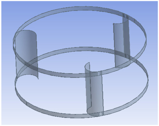
Figure 1.
C-blade rotor.

Table 1.
C-blade rotor values.
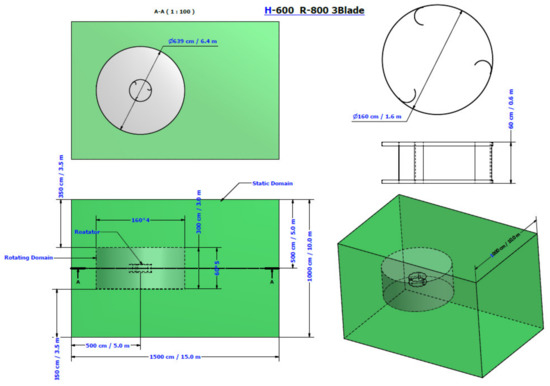
Figure 2.
Case 1: Geometry H-type C-blade (drag force) rotor.
2.2. Case 2: Involute Blade (Lift Force) Type Rotor
In this configuration, three involute shaped blades are placed 120° from each other with 180° blade openings. The blade chord length, blade height, and aspect ratio are fixed similarly to the previous case and the complete geometry of the configuration is presented in Figure 3. The geometrical values of the rotor configurations are listed in Table 2. Further, the calculated solidity (σ) of this configuration is about 3.43.
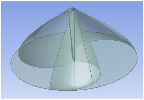
Figure 3.
Involute rotor type blades profile.
Table 2.
Involute rotor blade dimensions.
Figure 4 represents the comprehensive description of the involute-type rotor assembly and is uploaded in the ANSYS Fluent design modeler for the simulation.
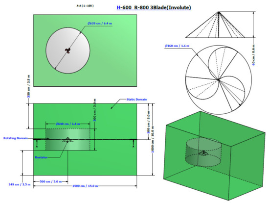
Figure 4.
Case 2: Geometry of involute-type rotor.
2.3. Case 3: Involute-Type Rotor with WFM
The physical configuration and simulation parameters are similar to the previous case, but there is an addition of WFM placed in front of the VAWT model in the direction of the wind velocity inlet. It consists of 0.6 m diffuser tubes with 0.3 m diameter towards the inlet side of the static domain and 0.15 m diameter towards the turbine side. The diffusers are arranged in a stack of 4 rows and 3 columns with decreasing diameter towards the VAWT Model. The decreasing cross-sectional area for wind flow in the tubes increases the pressure so that it accelerates wind velocity in the direction of wind flow. This simulation study carried out with rectangular-type WFM catches the wind from the proposed direction, and a circular-type WFM could be a future scope analysis, as it can catch wind from all directions. The physical description of rectangular and circular WFM are shown in Figure 5a,b.
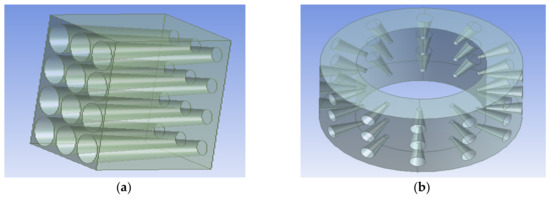
Figure 5.
Rectangular (a) and circular (b) wind flow modifier.
The height, width, and length are scaled as 1.4, 1.0, and 0.6 m, respectively. Additionally, the outer and inner radius of the diffuser are arranged as 0.03 and 0.015 m, respectively. The AutoCAD geometry of the diffuser consists of 12 tubes as shown in Figure 6 and adapted for the simulation process.
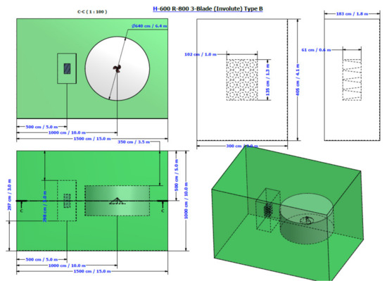
Figure 6.
Involute-type blade with WFM.
The VAWT turbine is modeled for the simulation study. All proposed designs are uploaded in the ANSYS tool to study the performance of the described cases.
3. Numerical Solution Methods
The physical modeling of the different configurations is discussed above. In this section, the mathematical modeling for all three cases is derived as follows.
3.1. General Governing Equations
The wind flow in a vertical axis wind turbine is a complex one [31] because of the wake flow [32,33] around the rotor blades. It necessitates CFD analysis along with a suitable turbulence model in the ANSYS Fluent tool to calculate preferred time-averaged velocity information to understand flow across the wind turbine. The incompressible (air) fluid flow (fluid density ρ is constant, independent of space and time) expressed with the continuity equation in mass conservation is described in Equation (1). Similarly, the Navies Stokes equation for momentum conservation is expressed in Equation (2). These solutions utilize the finite volume method [34,35].
3.2. Selection of Turbulence Model
The realizable k-ε turbulence model of the second-order upwind scheme with the SIMPLE segregated algorithm method [36] is applied to solve the Reynolds-averaged Navier Stokes (RANS) equations. The realizable k-ε turbulence model [37,38] with scalable wall function is a starting method for turbulence analysis for more accuracy and better convergence characteristics [39,40] for calculating power and torque, apart from its coefficient values for a VAWT model. The SIMPLE algorithm [41] is a pressure velocity coupling solution scheme, used to update the pressure and velocity in the simulation for better accuracy. The turbulence kinetic energy (k) and its dissipation rate (ε) for the realizable k-ε model are obtained from the following transport equations
where the terms C1, η, s, and pk are derived as follows,
where terms the generation of turbulence kinetic energy due to mean velocity gradients, defines the turbulence kinetic energy due to buoyancy, represents the contribution of the fluctuating dilatation incompressible turbulence to the overall dissipation rate, and are user-defined source terms, and are the turbulent Prandtl numbers for k and ε, and represents the kinematic viscosity of the fluid.
For improved accuracy, the double-precision [42] option is selected with second-order upwind-based discretization to compute the mean flow, turbulence, and transition equations. In this simulation, ρ = Air density (1.225 ), μ = Eddy viscosity ratio = 0.09, and the empirical constants = 1.43, = 1.92, and = 1.0, = 1.3 are input to the software.
3.3. Wind Turbine Governing Equations
The wind turbine governing equations for the power extraction from wind velocity [16,43] are represented by the following equation
where: P = power, F = Force vector, and V = velocity moving on wind turbine blades.
The wind power generation is , and swept area is where H = diameter of the turbine and H = height.
From the Betz limit for maximum power
The lift force and lift coefficient given as
The drag force and the drag coefficient
where: = torque coefficient
Before the start of the simulation, common rotor configurations are updated for all cases. Hence, the height (H) and diameter for the wind turbine are fixed as 0.6 and 1.6 m, respectively, to maintain the common aspect ratio of 0.75. It is already stated that an optimum number of blades for all three cases are chosen as 3 and the azimuth angle (α) is maintained at 90° (at which maximum power coefficient occurs). Additionally, the blades are exposed at 180° to the direction of the wind.
4. Computational Arrangement for the Simulation
The computational arrangement of the rotor, stator, VAWT, and WFM are described in the following sections.
4.1. Computational Domain
The computational domain consists of the stator domain, rotor domain, and wind turbine. The stator domain consists of a velocity inlet and pressure outlet with static wall surfaces and dimensions as shown in Figure 2, Figure 4, and Figure 6. The rotating domain consists of a wind turbine placed with + Z-axis (Figure 7). The length of the stator domain is fixed as 10D and width as 8D of the turbine diameter D [27]. The inlet is fixed with 2 m/s wind velocity, and the pressure outlet is fixed with zero pascal excess pressure assumed constant pressure at the outlet for all three cases. The rotating domain and turbine are bounded in a sliding mesh contact zone, and a suitable interface zone is also created to simulate the wind turbine rotation in different angular velocities (ω). In this configuration, the rotor domain is considered as a contact body and the wind turbine acts as a tool body.
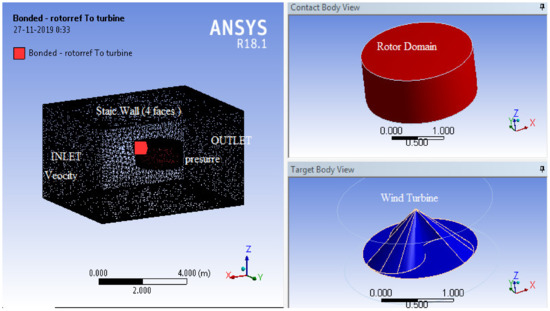
Figure 7.
Computational domain defined in ANSYS design modeler.
4.2. Computational Meshing
The geometry files are embedded into the design modeler for the proper domain separation, and later these arrangements are allowed into meshing mode. It is the time-consuming part of the software analysis, because the entire model is segregated into smaller mesh elements, which lead to better convergence characteristics. The improper meshing leads to early divergence in the final simulation. In this analysis, body sizing, refinement, and face sizing are the techniques followed for the proper meshing of domains. Tetrahedral cells and a significant element size were chosen for the wind turbine blade, which varies between 0.0005 and 0.005 m for better convergence. In the static domain, the meshing size reduced at 0.005 m. The details of all the meshed domains are shown in Figure 8 and Figure 9. The numbers of nodes and elements and cell skewness details are listed in Table 3.
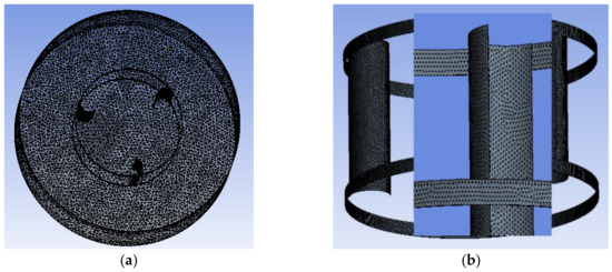
Figure 8.
Rotor domain (a) and C-shaped turbine (b). H-type rotor C-shaped blades mesh distribution.
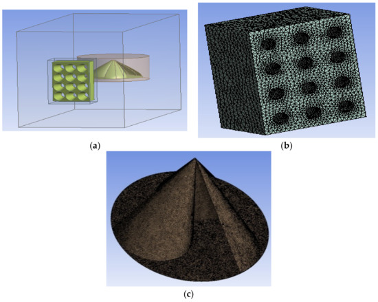
Figure 9.
Stator domain geometry (a), wind flow modifier (b) and involute rotor blades (c). Involute-type rotor with wind flow modifier (WFM) mesh distribution.
Table 3.
Meshing details of the three configurations.
4.3. Computational Solution Setup
The pressure velocity coupling model uses least squares cell-based gradient solution methods with first order, using implicit transient formulation. The moment or torque is calculated in second-order upwind discretization. The sliding mesh technique capable of giving good convergence characteristics is used to describe the rotor rotation. Turbulence is described with a realizable k-ε turbulence model with a SIMPLE segregated algorithm. The sliding mesh technique calculates the time step size [27] using Equation (20).
It is fixed that the maximum speed of the rotor for this simulation is 250 rpm by considering the diameter of the turbine comprises of 21 m/s linear velocity. Additionally, the minimum velocity is fixed as 5 m/s at 60 rpm, and the maximum angular velocity for the corresponding step size would be 0.0012 s [31]. In this work, the step size of 0.0001 is used in all three case studies for the common convergence characteristics. Additionally, the hybrid initialization method is used with the convergence target of 1 × 10⁻⁶ with 20 numbers of time steps. The maximum number of iterations is 10 per time step and implemented in the solution mode. As expected, the turbulence model gives better convergence characteristics with 100–150 iterations. All three proposed case studies are performed to set with 2 m/s wind velocity at inlet, and the angular velocity of the turbine varied from 60 to 250 rpm on the blades, which includes a linear velocity range of 5 to 21 m/s cutout speed. The performance characteristics of the H-type and involute turbines are examined. The parameters, such as lift and drag forces, their coefficients, momentum, torque, power, and power coefficients, are analyzed to identify the powerful wind turbine for low wind profile areas.
5. Simulation Results
This section describes the performance of proposed configurations for different wind velocities. The corresponding pressure variations on individual blades and the VAWT model, particularly on velocity variation starting from 2 m/s cut-in speed to 24 m/s cut out speed, are presented. This pressure variation creates drag and lift forces on the blades. The measure of drag and lift force coefficients and the related forces can give significant results for the proposed involute blades VAWT model. In addition to this, the electrical and mechanical characteristics of the blades and turbine model are also compared and investigated. To perform the simulation results, the velocity inlet is fixed at 2 m/s and the swept area scaled at 0.96 square meters for an optimal three-bladed turbine with appropriate domain specifications and sliding mesh rotor interfaces. The results of the different arrangements are discussed as follows.
5.1. Case 1: C-Shaped H-Type
The C-blade profiles are exposed to the –X axis velocity inlet direction. Further, the profiles are studied through the pressure contours, and drag and lift forces exerted on the blades are studied at 60 rpm angular velocity, which is equivalent to 5 m/s (linear velocity for the corresponding diameter). Since this configuration consists of an optimal three-blade turbine, the individual pressure and velocity performance of each blade is performed below.
5.1.1. Individual Blade Performance
The pressure variations exposed on the C-blades state that Blade 3 predominantly creates a high amount of negative pressure (−181 Pa) and exerts more drag force, followed by Blade 1. In contrast, Blade 2 generates high pressure but with less drag force on the +Z rotational axis, as shown in Figure 10. Blade 3 generates high drag force, followed by Blade 1, and the net drag coefficient (Cd = 0.205) obtained much higher than the negative lift coefficient (Cl = −0.094), as shown in Figure 11. Moreover, it is found that the C-shaped blades rotate the turbine rotor by a drag force, and the ratio of drag to lift force obtained a scale of 2.181 at 60 rpm.
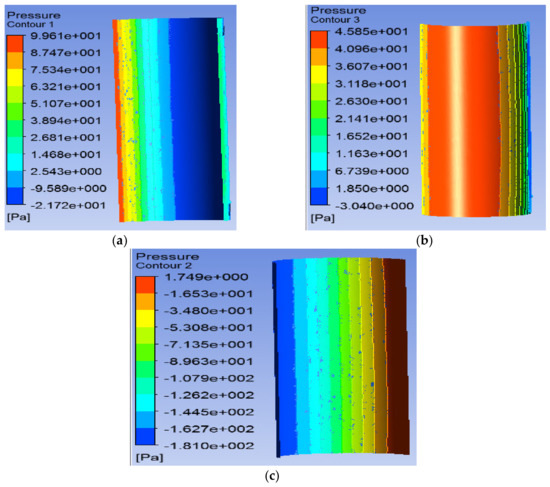
Figure 10.
Blade 1 (a), blade 2 (b) and blade 3 (c). C- shaped H- type pressure contours.
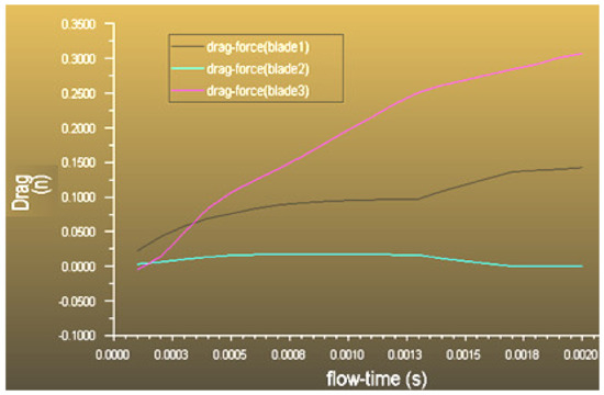
Figure 11.
Drag characteristics (Cd).
5.1.2. Rotor Performance
The rotor performance of the C-blade at 60 rpm wind velocity is depicted in this section. It is stated that in the above sections, the main objective of this work is to identify low-velocity wind turbines. Therefore, it is imperative to determine the pressure and velocity variations, velocity gradient between inlet and turbine, and momentum coefficient.
In a C-blade turbine, Blade 2 generates high pressure of +99.6 Pa, and Blade 1 generates −21 Pa, as shown in Figure 12. Therefore, high velocity is attained at the tip of Blade 1, as presented in Figure 13, which consequences the highest torque exerted on it. However, the resultant drag forces cause the rotor to rotate in a counterclockwise direction, that is, from Blade 2 to Blade 1, as per the direction shown in Figure 14. It shows that the lift forces are perpendicular to wind velocity and the drag forces in the direction of relative wind velocity. The moment value from the simulation results is obtained to study the torque characteristics of the blades and the turbine, which is measured from the reference +Z rotational axis. It is found that Blade 1 generated the maximum moment of 0.3 at a low negative pressure (Figure 15). In contrast, the other two blades generate negative momentum, and hence reduce the net resultant torque. This might be one of the important reasons for the low power generation from drag force-based wind turbines.
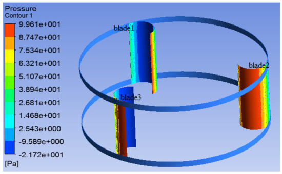
Figure 12.
Pressure variation over the rotor.
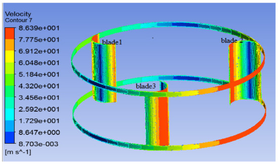
Figure 13.
Velocity variation over the rotor.
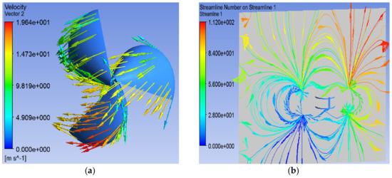
Figure 14.
(a) Lift and drag Forces; (b) velocity gradients.
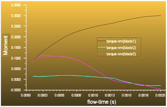
Figure 15.
Blade momentum.
5.2. Case 2: Involute Type
The newly proposed conical involute-shaped rotor blades are shown in Figure 3; their dimensional values are given in Table 2. This involute blade shape consists of a spline radius of 1.1 per mm; minimum curvature of 0.0024 per mm and a maximum curvature of 1.8 per mm are considered. Additionally, a minimum face angle of 10° and a maximum of 174° are constructed for this simulation in –X axis. It is believed that the conical outer surface of this model may produce supporting lift forces along with the drag forces that are always available in the room of involute shapes. This particular property may improve VAWT model performances.
5.2.1. Individual Blade Performance
The individual blade of the conical-shaped involute configuration generates more lift forces on its surfaces. Unlike C-shaped blades, the voluminous design inside the blades generates drag forces and aids the turbine to rotate. In the principles of aerodynamics, the profiles move from high pressure to low pressure [44]; hence, the pressure variation on Blade 2 occurred between +482 and −104 Pa, as illustrated in Figure 16. It generates lift coefficients of −0.272 (negative sign shows force acts in the downward direction) on Blade 2 and results in a net lift coefficient (Cl) of −0.554 (Table 4).
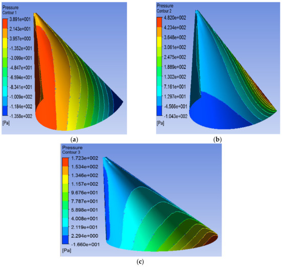
Figure 16.
Blade 1 (a), blade 2 (b) and blade 3 (c). Involute-type pressure contours.
Table 4.
Lift and drag coefficients.
Additionally, the negative drag coefficient (−0.00375) supports the lift forces and is prompted to obtain a net lift coefficient much higher than the drag coefficient. This shows that the proposed involute-shaped blades rotate the turbine rotor by lift force due to the higher ratio of lift to drag (14.02) originated at even at 60 rpm. This ratio of lift to drag with C-shaped blades at 60 rpm is . This force ratio index indicates the effectiveness of the proposed involute blades in the VAWT model.
5.2.2. Rotor Performance
In this case, involute rotor blade 1 generates high pressure of +480 Pa and low pressure −135 Pa at Blade 2, as shown in Figure 17. This results in a high velocity of about 15.34 ms−1, as illustrated in Figure 18a, and high torque at Blade 2.
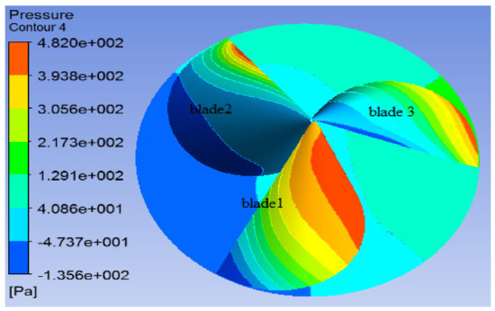
Figure 17.
Pressure variation over the rotor.

Figure 18.
Velocity (a) and gradient (b) variations on involute blades.
Figure 18b exhibits the velocity gradients from inlet to outlet of the turbine model. A velocity gradient is a measure of velocity variations that happened between inlet and outlet for the involute case. Further, involute turbines generate only positive moments from all three blades; consequently, this increases the resultant torque, as shown in Figure 19. The moment generated by the involute blade is 6.82 times higher than the C-blade rotor.
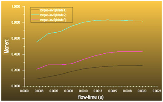
Figure 19.
Blade momentum.
5.3. Case 3: Involute-Type Rotor with WFM
The WFM was constructed with a stack of 12 diffuser tubes (4 rows, 3 columns) with an inlet to outlet diameter variation about 2 times. It exhibits pressure variations between +465 and −19.3 Pa, as shown in Figure 20a. This pressure variation from high pressure to low pressure in the diffuser tubes generates velocity variations of approximately from 1.822 m/s (inlet) to 5.562 m/s (outlet) with the velocity magnification ratio of 3.05. It aids in achieving more forces on the turbine, as shown in Figure 20b. The changes in the velocity amplification from inlet to the outlet of the diffuser tubes signify the use of the additional benefits of this model for low wind profile areas. This WFM and VAWT model signifies condenser and turbine connection in thermal power plant for steam energy conversion.
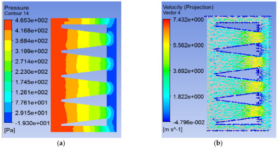
Figure 20.
Pressure (a) and velocity (b) variations inside the diffuser tubes.
5.3.1. Individual Blade Performance
The effect of the wind flow modifier (WFM) exerting the pressure variations on the involute blades is presented in Figure 21. This configuration is similar to case 2 but with the additional placement of the wind flow modifier between inlet and turbine, resulting in a higher rate of pressure variations over the blade surfaces. Particularly, Blade 1 shows intensified low-pressure variations of −228 Pa and generates a higher lift force than the other two blades. Unlike the previous case, all three blades are contributing an equal amount of lift forces, as shown in Table 5. This results in the highest lift coefficient of about 0.33, 0.32, and 0.22 at Blade 1, Blade 2, and Blade 3, respectively. Additionally, the lift to drag ratio is improved to 18.84 by placing the WFM in the direction of the wind.
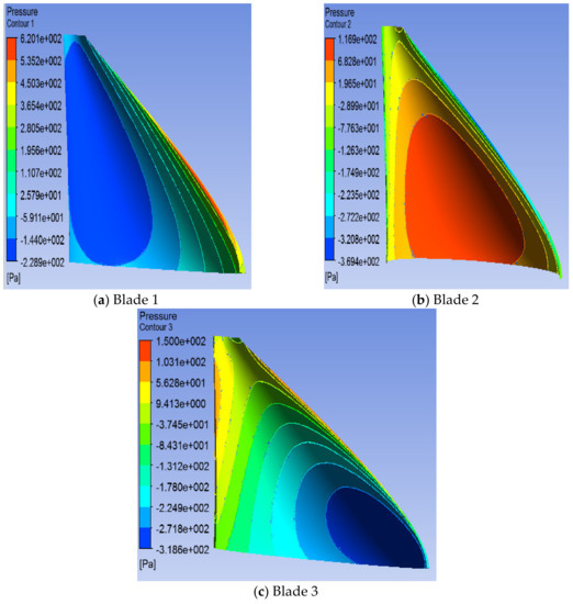
Figure 21.
Blade 1 (a), blade 2 (b) and blade 3 (c). Involute type with WFM pressure contours.
Table 5.
Lift and drag coefficients.
5.3.2. Rotor Performance
In this configuration, the rotor with WFM generates high and low pressure of about +150 and −318 Pa, respectively, as presented in Figure 22. Further, the velocity range exerted on the rotor is about 16.57 ms−1, resulting in a higher torque rate compared with previous case studies (Figure 23).
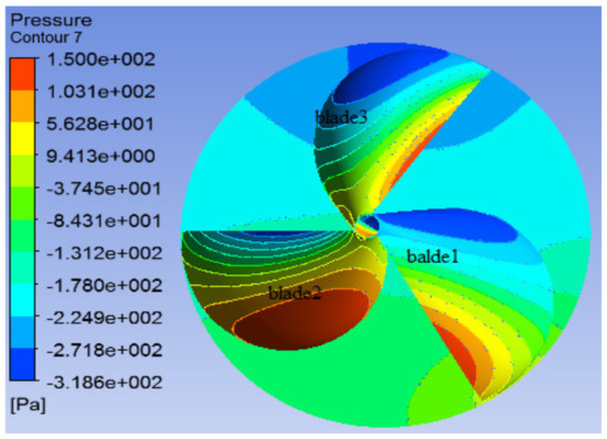
Figure 22.
Pressure contour.
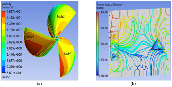
Figure 23.
Velocity (a) and gradient (b) variations on involute blades with WFM.
The moment generated by the WFM-based rotor is 1.56 times higher than the involute rotor, as illustrated in Figure 24. The overall performance of all three configurations has been discussed using the simulation results. It is found that the involute rotor with WFM configuration offers improved performance. However, the electrical and mechanical characteristics of the configurations have to be appropriately designed, as discussed next.
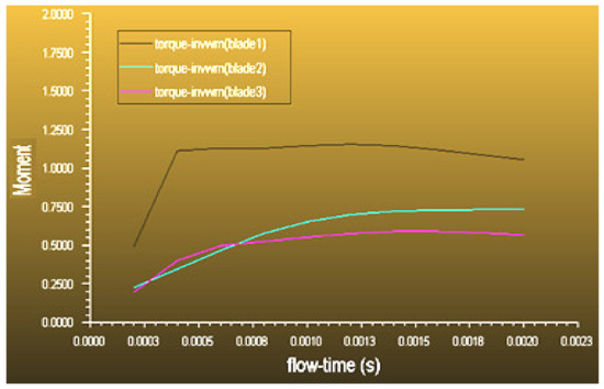
Figure 24.
Blade momentum.
6. Discussions on Electrical and Mechanical Features
This section describes the electrical and mechanical characteristics of all three proposed case studies. Simulations are performed at a predefined angular velocity of the turbine and attempt to identify the most effective configuration for a range of wind velocities. The VAWT model is exposed to 60, 125, 180, and 250 rpm, which is equivalent to 5, 10, 15, and 21 m/s in linear velocity [22]. Normally, the cut-out speed of the VAWT model is in the range of 20 m/s. Further, mechanical parameters such as torque, lift, and drag forces and their coefficients are identified for all the angular velocities. Subsequently, electrical parameters, such as power and its coefficient, are also determined for the minimum to maximum angular velocities.
6.1. Mechanical Characteristics
Lift to drag coefficient (drag to lift in the case of the C-blade model) is a significant aerodynamic factor. It completely expresses the mechanical performances of a VAWT model. Additionally, the higher value of this ratio signifies a better power coefficient for a wind turbine. The C-blade H-type model maintains a much lower lift to drag ratio, varying from 2.181 to 2.553 for all proposed wind velocities. On the other hand, in Case 2 with the involute rotor, this ratio increased to 14.02 significantly at low wind velocity, and it decreased with an increase in angular velocity due to increased unsupported drag forces.
For Case 3, the minimum lift to drag ratio is 18.44 obtained at 60 rpm, and it increases to the highest value of 31.44 at 250 rpm (Figure 25). Hence, the addition of WFM effectively improves the aerodynamic forces of the wind turbine; therefore, WFM-based wind turbines would be a great choice for all kinds of wind velocity if the WFM could be turned in the direction of wind flow. The numerical data of all three configurations are given in Table 5.
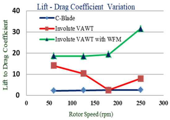
Figure 25.
Mechanical characteristics.
6.2. Electrical Characteristics
The net torque (Nm) obtained through the simulation for various wind velocities is converted into electrical power (watt) using Equation (18) and the power coefficient calculated from Equation (19). The computed values are tabulated in Table 6, and the rotor power and power coefficient are plotted in Figure 26. It exhibits that the VAWT model with WFM provides the maximum power coefficient of 0.397 at 60 rpm.
Table 6.
Performance details of all three cases.
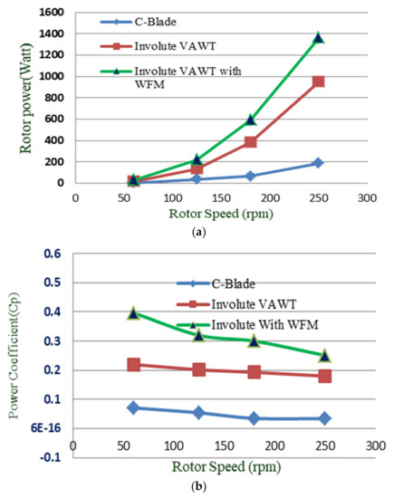
Figure 26.
Electrical characteristics: (a) rotor power and (b) power coefficient.
The tabulated result shows that the involute model can generate 1.361 kW at 21 m/s wind velocity. In contrast, the drag-based wind turbine exhibits a reduced power conversion ratio for all velocity ranges. The C-shaped blades can produce only a maximum of 188.8 W at 250 rpm (26.17 rad/s). The electrical power of the other two configurations is 951 W and 1361 W, which is very significant in the energy conversion through VAWT model configuration.
From the observed results, it is observed that the power coefficient () values obtained for case 3 show greater value with a maximum of 0.397 and a minimum of 0.29 compared to the other two cases. Hence the involute-type turbine model with a wind flow modifier can be adapted for all kinds of wind velocities, particularly low wind velocity zones.
7. Conclusions
This work proposes three different rotor configurations for the VAWT model for a low wind urban area. It is structured in a realizable k-ε turbulence model in ANSYS Fluent software. This model gives better convergence characteristics and reliable results for all three different rotor configurations. From the simulation results, it is found that the proposed WFM-based VAWT model intensifies the wind velocity in its outlet before it reaches the turbine blades. It provides potential benefits as follows.
- The lift—drag coefficient displays a greater value of about 19 at 60 rpm and 30 during 250 rpm, which is comparatively superior to other configurations.
- The addition of WFM effectively increases the aerodynamic forces of the wind turbine for all kinds of wind velocity.
- The WFM model with an involute rotor generates a maximum of 1361 watts during the wind velocity of 250 rpm.
- The power coefficient of this model is significantly enhanced up to approximately 0.397, even at low wind velocity.
Hence, the WFM-based involute rotor VAWT model shows superior mechanical and electrical wind energy conversion characteristics compared to other configurations. Therefore, this WFM with involute VAWT model configuration may potentially be used for generating electrical energy in low wind profile areas, particularly in urban regions. Also, it will be useful for optimal planning of wind farm [45] or microgrid [46].
Author Contributions
Conceptualization: M.A.; methodology: M.A.; software: M.A.; validation: V.P.; formal analysis: V.P.; data curation: K.R.; writing—original draft preparation: K.R.; writing—review and editing: M.H.A.; supervision: Z.W.G. and J.H.; funding acquisition: Z.W.G. and J.H. All authors have read and agreed to the published version of the manuscript.
Funding
This research was supported by the Energy Cloud R&D Program through the National Research Foundation of Korea (NRF) funded by the Ministry of Science, ICT (2019M3F2A1073164).
Conflicts of Interest
The authors declare no conflict of interest.
References
- Blakers, A.; Stocks, M.; Lu, B.; Cheng, C.; Stocks, R. Pathway to 100% Renewable Electricity. IEEE J. Photovoltaics 2019, 9, 1828–1833. [Google Scholar] [CrossRef]
- Krishnamoorthy, R.; Udhayakumar, K.; Kannadasan, R.; Elavarasan, R.M.; Mihet-Popa, L. An Assessment of Onshore and Offshore Wind Energy Potential in India Using Moth Flame Optimization. Energies 2020, 13, 3063. [Google Scholar]
- Madurai Elavarasan, R.; Selvamanohar, L.; Raju, K.; Vijayaraghavan, R.R.; Subburaj, R.; Nurunnabi, M.; Khan, I.; Afridhis, S.; Hariharan, A.; Pugazhendhi, R.; et al. A Holistic Review of the Present and Future Drivers of the Renewable Energy Mix in Maharashtra, State of India. Sustainability 2020, 12, 6596. [Google Scholar] [CrossRef]
- Patnaik, K.; Samantaray, B. A Study of Wind Energy Potential in India. Bachelor’s Thesis, Department of Electrical Engineering, National Institute of Technology, Rourkela, India, 2010. [Google Scholar]
- Lakshmanan, N.; Gomathinayagam, S.; Harikrishna, P.; Abraham, A.; Ganapathi, S.C. Basic wind speed map of India with long-term hourly wind data. Curr. Sci. 2009, 96, 911–922. [Google Scholar]
- Majdi Nasab, N.; Kilby, J.; Bakhtiaryfard, L. The Potential for Integration of Wind and Tidal Power in New Zealand. Sustainability 2020, 12, 1807. [Google Scholar] [CrossRef]
- Zuo, H.; Bi, K.; Hao, H. A state-of-the-art review on the vibration mitigation of wind turbines. Renew. Sustain. Energy Rev. 2020, 121, 109710. [Google Scholar] [CrossRef]
- Pustina, L.; Lugni, C.; Bernardini, G.; Serafini, J.; Gennaretti, M. Control of power generated by a floating offshore wind turbine perturbed by sea waves. Renew. Sustain. Energy Rev. 2020, 132, 109984. [Google Scholar] [CrossRef]
- Mohammed, A.A.; Ouakad, H.M.; Sahin, A.Z.; Bahaidarah, H.M.S. Vertical axis wind turbine aerodynamics: Summary and review of momentum models. J. Energy Resour. Technol. 2019, 141, 050801. [Google Scholar] [CrossRef]
- Deng, W.; Yu, Y.; Liu, L.; Guo, Y.; Zhao, H. Research on the dynamical responses of H-type floating VAWT considering the rigid-flexible coupling effect. J. Sound Vib. 2020, 469, 115162. [Google Scholar] [CrossRef]
- Kumar, R.; Raahemifar, K.; Fung, A.S. A critical review of vertical axis wind turbines for urban applications. Renew. Sustain. Energy Rev. 2018, 89, 281–291. [Google Scholar] [CrossRef]
- Wang, K.; Zou, L.; Wang, A.; Zhao, P.; Jiang, Y. Wind Tunnel Study on Wake Instability of Twin H-Rotor Vertical-Axis Turbines. Energies 2020, 13, 4310. [Google Scholar] [CrossRef]
- Viqueira-Moreira, M.; Ferrer, E. Insights into the Aeroacoustic Noise Generation for Vertical Axis Turbines in Close Proximity. Energies 2020, 13, 4148. [Google Scholar] [CrossRef]
- Niranjana, S.J. Power Generation by Vertical Axis Wind Turbine. Int. J. Emerg. Res. Manag. Technol. 2015, 7, 1–7. [Google Scholar]
- Naseem, A.; Uddin, E.; Ali, Z.; Aslam, J.; Shah, S.R.; Sajid, M.; Zaidi, A.A.; Javed, A.; Younis, M.Y. Effect of vortices on power output of vertical axis wind turbine (VAWT). Sustain. Energy Technol. Assess. 2020, 37, 100586. [Google Scholar] [CrossRef]
- Li, Z.; Han, R.; Gao, P.; Wang, C. Analysis and implementation of a drag-type vertical-axis wind turbine for small distributed wind energy systems. Adv. Mech. Eng. 2019, 11, 1–16. [Google Scholar] [CrossRef]
- Sobczak, K.; Obidowski, D.; Reorowicz, P.; Marchewka, E. Numerical Investigations of the Savonius Turbine with Deformable Blades. Energies 2020, 13, 3717. [Google Scholar] [CrossRef]
- Mauri, M.; Bayati, I.; Belloli, M. Design and realisation of a high-performance active pitch-controlled H-Darrieus VAWT for urban installations; CP651. In Proceedings of the 3rd Renewable Power Generation Conference (RPG 2014), Naples, Italy, 24–25 September 2014. [Google Scholar]
- Su, H.; Dou, B.; Qu, T.; Zeng, P.; Lei, L. Experimental investigation of a novel vertical axis wind turbine with pitching and self-starting function. Energy Convers. Manag. 2020, 217, 113012. [Google Scholar] [CrossRef]
- Kavade, R.K.; Ghanegaonkar, P. Design and Analysis of Vertical Axis Wind Turbine for Household Application. J. Clean Energy Technol. 2017, 5, 353–358. [Google Scholar] [CrossRef]
- Tirkey, A.; Sarthi, Y.; Patel, K.; Sharma, R.; Sen, P.K. Study on the effect of blade profile, number of blade. Int. J. Sci. Eng. Technol. Res. 2014, 3, 3183–3187. [Google Scholar]
- Mohanasundaram, A.; Valsalal, P. Analysis and design of vertical axis wind turbine for a low wind profile urban areas. J. Electr. Eng. 2019, 20, 363–375. [Google Scholar]
- Yi, M.; Jianjun, Q.; Yan, L. Airfoil Design for Vertical Axis Wind Turbine Operating at Variable Tip Speed Ratios. Open Mech. Eng. J. 2018, 9, 1007–1016. [Google Scholar] [CrossRef]
- Biadgo, A.M.; Simonović, A.; Komarov, D.; Stupar, S. Numerical and analytical investigation of vertical axis wind turbine. FME Trans. 2013, 41, 49–58. [Google Scholar]
- Suffer, K.H.; Quadir, G.A.; Ismail, K.A.; Ryspek, U. CFD analysis of three and four blades movable vanes type vertical axis wind turbine having movable vanes. Int. J. Smart Grid Clean Energy 2016, 5, 259–263. [Google Scholar] [CrossRef]
- Franchina, N.; Kouaissah, O.; Persico, G.; Savini, M. Three-Dimensional CFD Simulation and Experimental Assessment of the Performance of a H-Shape Vertical-Axis Wind Turbine at Design and Off-Design Conditions. Int. J. Turbomach. Propuls. Power 2019, 4, 30. [Google Scholar] [CrossRef]
- Alaimo, A.; Esposito, A.; Messineo, A.; Orlando, C.; Tumino, D. 3D CFD Analysis of a Vertical Axis Wind Turbine. Energies 2015, 8, 3013–3033. [Google Scholar] [CrossRef]
- D’souza, A.G.; Concessao, J.I.; Quadros, J. Study of Aerofoil Design Parameters for Low Speed Wind Tunnel. J. Mech. Eng. Autom. 2015, 5, 47–54. [Google Scholar]
- Zhu, H.T.; Hao, W.X.; Li, C.; Ding, Q.W. Impact of Solidity on Aerodynamic Performance of Building Augmented Vertical Axis Wind Turbine. Reneng Dongli Gongcheng J. Eng. Therm. Energy Power 2018, 33, 114–121. [Google Scholar]
- Sun, X.; Zheng, Z.; Huang, D.; Chen, Y.; Cao, Y.; Wu, G. Research on the aerodynamic characteristics of a lift drag hybrid vertical axis wind turbine. Adv. Mech. Eng. 2016, 8, 1687814016629349. [Google Scholar] [CrossRef]
- Rezaeiha, A.; Kalkman, I.; Blocken, B. Effect of pitch angle on power performance and aerodynamics of a vertical axis wind turbine. Appl. Energy 2017, 197, 132–150. [Google Scholar] [CrossRef]
- Mendoza, V.; Goude, A. Wake Flow Simulation of a Vertical Axis Wind Turbine Under the Influence of Wind Shear. J. Phys. Conf. Ser. 2017, 854, 12031. [Google Scholar] [CrossRef]
- Reitz, A.R.; Yan, C.R.; Ogle, J.; Seel, P. Computational Modeling of Wind Turbine Wake Interactions. Master’s Thesis, Colorado State University, Fort Collins, CO, USA, 2012. [Google Scholar]
- Rezaeiha, A.; Montazeri, H.; Blocken, B. Towards optimal aerodynamic design of vertical axis wind turbines: Impact of solidity and number of blades. Energy 2018, 165, 1129–1148. [Google Scholar] [CrossRef]
- Turbulence Models in ANSYS® Fluent CFD. Available online: https://davis68.github.io/me498cf-fa16/resources/flec06/handout-turbulence.pdf (accessed on 28 August 2020).
- Muiruri, P.I.; Motsamai, O.S. Three Dimensional CFD Simulations of A Wind Turbine Blade Section; Validation. J. Eng. Sci. Technol. Rev. 2018, 11, 138–145. [Google Scholar] [CrossRef]
- Liang, Y.B.; Zhang, L.X.; Li, E.X.; Zhang, F.Y. Blade pitch control of straight-bladed vertical axis wind turbine. J. Cent. South Univ. 2016, 23, 1106–1114. [Google Scholar] [CrossRef]
- Mohamed, M.; Ali, A.; Hafiz, A. CFD analysis for H-rotor Darrieus turbine as a low speed wind energy converter. Int. J. Eng. Sci. Technol. 2014, 18, 1–13. [Google Scholar] [CrossRef]
- Prasad, D.; Ratkovich, N.R.; Kirkegaard, P.H.; Nielsen, S.R. Design of rotor blade for vertical axis wind turbine using double aerofoil. In Proceedings of the International Conference on Wind Energy: Materials, Engineering, and Policies (WEMEP 2012), Hydrabad, India, 22–23 November 2012. [Google Scholar]
- Pujol, T.; Massaguer, A.; Massaguer, E.; Montoro, L.; Comamala, M. Net Power Coefficient of Vertical and Horizontal Wind Turbines with Crossflow Runners. Energies 2018, 11, 110. [Google Scholar] [CrossRef]
- Kao, J.-H.; Tseng, P.-Y. Application of computational fluid dynamics (CFD) simulation in a vertical axis wind turbine (VAWT) system. IOP Conf. Series: Earth Environ. Sci. 2018, 114, 12002. [Google Scholar] [CrossRef]
- Reddy, K.; Dagamoori, K.; Sruthi, A.P.; Apurva, S.N.; Naidu, N.M.L. A Brief Research, Study, Design and Analysis on Wind turbine. J. Mod. Eng. Res. 2015, 5, 26. [Google Scholar]
- Jain, P.; Abhishek, A. Analysis and prediction of Vertical cycloidal Rotor Wind Turbine with variable amplitude pitching. In Proceedings of the ARF 2015—4th Asian-Australian Rotorcraft Forum, Bengaluru, India, 16–18 November 2015; pp. 5–7. [Google Scholar]
- Rathod, V.K.; Kamdi, S.Y. Design of PVC Bladed Horizontal Axis Wind Turbine for Low Wind Speed Region. J. Eng. Res. Appl. 2014, 4, 139–143. [Google Scholar]
- Geem, Z.W.; Hong, J. Improved Formulation for the Optimization of Wind Turbine Placement in a Wind Farm. Math. Probl. Eng. 2013, 2013, 481364. [Google Scholar] [CrossRef]
- Geem, Z.W. Size Optimization for a Hybrid Photovoltaic-Wind Energy System. Int. J. Electr. Power Energy Syst. 2012, 42, 448–451. [Google Scholar] [CrossRef]


© 2020 by the authors. Licensee MDPI, Basel, Switzerland. This article is an open access article distributed under the terms and conditions of the Creative Commons Attribution (CC BY) license (http://creativecommons.org/licenses/by/4.0/).