An Analysis of the Interactions between Adjustment Factors of Saturation Flow Rates at Signalized Intersections

Abstract

An insufficient functional relationship between adjustment factors and saturation flow rate (SFR) in the U.S. Highway Capacity Manual (HCM) method increases an additional prediction bias. The error of SFR predictions can reach 8–10%. To solve this problem, this paper proposes a comprehensive adjusted method that considers the effects of interactions between factors. Based on the data from 35 through lanes in Beijing and 25 shared through and left-turn lanes in Washington, DC, the interactions between lane width and percentage of heavy vehicles and proportion of left-turning vehicles were analyzed. Two comprehensive adjustment factor models were established and tested. The mean absolute percentage error (MAPE) of model 1 (considering the interaction between lane width and percentage of heavy vehicles) was 4.89% smaller than the MAPE of Chinese National Standard method (Standard Number is GB50647) at 13.64%. The MAPE of model 2 (considering the interaction between lane width and proportion of left-turning vehicles was 33.16% smaller than the MAPE of HCM method at 14.56%. This method could improve the accuracy of SFR prediction, provide support for traffic operation measures, alleviate the traffic congestion, and improve sustainable development of cities.

1. Introduction

With the rapid development of economy and society, the number of vehicles has been increasing rapidly in developing countries such as China [1]. As a result, traffic congestions have become frequent. In 2018, the average daily congestion duration was nearly three hours in Beijing [2]. This trend has been spreading from large cities to small and medium-sized cities. The emission problems, which are caused by traffic jams, are growing worse. Traffic congestion has become a key problem that restricts the sustainable development of cities. Intersections where multiple traffic flows converge are the important nodes in the road network [3]. In addition, because the capacity of intersections is less than the capacity of road section, intersections often become bottlenecks of the road networks. Previous studies have shown that the capacity of intersections is less than 50% of the road sections, and the delay accounts for 80% of the road network. Concentrations of CO and NO_X exceed the National Air Quality Standard near signalized intersections during peak hours [4]. Because of idling, acceleration, and deceleration, the fuel consumption and emission of vehicles will inevitably increase at signalized intersections. It is becoming an important but difficult point how to improve the traffic capacity and alleviate the traffic congestion [5].

The primary cause of traffic congestion is unbalance between traffic supply and demand. In general, there are two ways to alleviate traffic congestion at signalized intersections. The first one is to improve traffic capacity with unique and refined design [6,7]. The second one is to decrease delay with optimization signal control [8,9]. All the methods need the guidance of capacity theory. The U.S. Highway Capacity Manual (HCM) states that the capacity theory can help engineers make the right decisions about operation, design, and planning according to different purposes [10]. Therefore, accurate capacity estimation of signalized intersections will play an important role in engineering applications.

Saturation flow rate (SFR) is one of the most important parameters in capacity estimation of signalized intersections. Saturation flow rate represents the maximum average hourly flow rate at which vehicles can pass through stop line if the signal is green at all times [10]. At present, there are two methods to estimate saturation flow rate. One is based on field measurements. The other one is based on model formula. The measurement process is based on the Highway Capacity Manual (HCM). Firstly, the fourth vehicle in the queue is recorded when the front axle crosses the stop line. Secondly, the last vehicle in the queue is also recorded. Thirdly, the time lag of the fourth and last vehicle is calculated. Fourthly, we can divide time lag by the number of vehicles to get saturation headway. Finally, saturation flow rate is the time reciprocal of the saturation headway. The model method is computed by the procedure described in HCM. The estimated saturation flow rate is determined by multiplying the base saturation flow rate (BSFR) by specific geometric and operational factors that affect the lane. The base saturation flow rate represents the saturation flow rate for a traffic lane that is 12 ft wide and has no heavy vehicles, a flat grade, no parking, no buses that stop at the intersection, even lane utilization, and no turning vehicles. The estimated saturation flow rate is generally applied in the design and management stages and verifies the feasibility of the solutions.

At present, most research is based on model method. The adjustment factors in Highway Capacity Manual (HCM) were modified according to the local traffic characteristics [11]. It could improve the estimation accuracy of saturation flow rate. However, many researchers found that there was still some error of estimation saturation flow rate when the adjustment factors were modified. The authors of the British [12] and Australian [13] methods admit a rather high standard error of saturation flow estimations reaching 8–10% [14]. This error may be caused by the structure of the multiplicative model. Hence, analysis of multiplicative model structure and the relationship between adjustment factors could improve the estimation accuracy of saturate flow rate, the decision-making ability of design and management, and reduce delays and emissions. It is very important for alleviating the traffic congestion and improving sustainable development of cities.

2. Literature Review

2.1. Existing Capacity Manuals for Signalized Intersections

In the world, the capacity analysis method of signalized intersections in different countries is based on U.S. Highway Capacity Manual (HCM) method. HCM has been updated five times so far [15]. The signalized intersection chapter has renewal in each version. However, the saturation flow rate (SFR) model is almost unchanged, as is shown in Equation (1). It consists of a multiplicative model that assumes the saturation flow effect of multiple non-ideal conditions is the product of all individual non-ideal factors. The saturation flow rate adjustment factors are primarily determined by isolating a single variable. The combination of multiple nonideal factors are largely unknown. The HCM considers that there are only 11 factors that affect saturation flow estimates. These factors are: lane width, heavy vehicles in traffic stream, approach grade, existence of a parking lane and parking activity adjacent to lane group, blocking effect of local buses that stop within intersection area, area type, lane utilization, left-turn vehicle presence in a lane group, right-turn vehicle presence in a lane group, pedestrian for left-turn groups, and pedestrian for right-turn groups.

$$s=s_0·f_w{f}_{HV}{f}_g{f}_p{f}_{bb}{f}_a{f}_{LU}{f}_{LT}{f}_{RT}{f}_{Lpb}{f}_{Rpb}$$

(1)

where, s is adjusted saturation flow rate (veh/h/ln), s₀ is base saturation flow rate (pcu/h/ln), and f is adjustment factors for various non-ideal geometric, traffic, and environmental conditions.

In Canada, the Committee on the Canadian Capacity Guide for Signalized Intersections has published the Canadian Capacity Guide for Signalized Intersections (CCG) in 2008 [16]. They have corrected minor errors in the Highway Capacity Manual (HCM) method. The saturation flow rate (SFR) estimation is the same as HCM method which is a multiplicative model. However, unlike HCM, the base saturation flow rate values are measured in nine Canadian cities. These include values for exclusive through lanes and exclusive left turn lanes in both suburban and downtown locations. The adjustment factors depend on the combination of intersection geometric, traffic, and control conditions. These are: lane width, grade, turning radius, queueing and discharge space, transit stops, parking, pedestrians, duration of green interval, protected left turns, permissive left turns, permissive left turns with pedestrians, right turns with pedestrians, and various shared lane combinations.

In Germany, Forschungsgesellschaft für Straßen- und Verkehrswesen (FGSV, Road Transport Research Institute) has drafted the latest German highway capacity manual which is Handbuch für die Bemessung von Straßenverkehrsanlagen (HBS) [17]. The saturation flow rate estimation is similar to Highway Capacity Manual (HCM) method. Saturation flow rate is also the time reciprocal of the saturation headway. The estimation of saturation headway is based on multiplicative model. The base saturation headway is 1.8 s. There are three adjustment factors that have effects on saturation headway: lane width, grade, and turning radius. Similarly, different formulas are used to estimate saturation headway for different lane combinations.

In India, the India Highway Capacity Manual (Indo-HCM) was written by the Council of Scientific and Industrial Research (CSIR) and seven other research institutes [18]. Moreover, in the case of existing signalized intersections, the users have the option of either using the models developed for the estimation of saturation flow and controlling delay or directly obtaining these parameters through field measurement procedures prescribed in Indo-HCM. Further, adjustment factors accounting for the ground conditions existing at any non-base intersections are also proposed in the manual which can be used to obtain the prevailing saturation flows and capacity. These are bus blockage, blockage by standing right-turn vehicles, and the initial surge of vehicles.

In China, Tongji University and 11 other institutes have compiled a Chinese National Standard that is code for planning of intersections on urban roads (Standard Number is GB50647-2011) [19]. It is used to guide the planning of intersections at urban planning. The saturation flow rate estimation is the same as Highway Capacity Manual (HCM) method. The base saturation flow rate measures values in three different types of cities which are located in eastern, western, and central China. There are four adjustment factors that affect the saturation flow rate: lane width, grade, percentage of different type vehicles, and turn radius.

2.2. Adjustment Factors

In order to improve the accuracy of capacity estimation, adjustment factors become the focus of research. The common adjustment factors include lane width, vehicle composition, and various shared lanes [20,21,22,23,24,25,26,27,28,29,30,31,32].

Now adjustment factors for lane width are discussed. The research on lane width has a long history. Initially, it was to study the highway lane width. Based on the survey data, the relationship model of lane width and speed is developed. It is found that lane width is positively correlated with saturation flow rate [20,21,22]. Zegeer et al. [20] studied the saturation flow rate at different scenarios in which the lane width of 2.6 to 4.7 m (8.5 to 15.5 ft). All baseline conditions, except for lane width, were held constant. The survey results were compared with those of the baseline condition surveys. The narrower lane widths demonstrated saturation flow rates from 2% to 5% lower than those in the baseline surveys, whereas the wider lane widths demonstrated saturation flow rates 5% higher. Potts et al. [21] studied the relationship between lane width and saturation flow rate on approaches at signalized intersections located downtown and in suburban areas. It is found that saturation flow rate varies with lane width. Average saturation flow rate was in the range of 1736–1913 passenger cars (pc)/h/ln for 2.9 to 4.0 m lanes. These measured saturation flow rates are generally lower than those currently used in the Highway Capacity Manual (HCM). However, these studies analyzed the relationship between lane width and saturation flow rate, lacking consideration of other adjustment factors.

Now adjustment factors for vehicle composition are discussed. Due to the difference in vehicle performance, based on measured data, estimation of passenger car unit (PCU) was analyzed. Further, adjustment factor for heavy vehicles was studied [23,24,25,26]. Radhakrishnan et al. [23] found that HCM has recommended a saturation flow model primarily for homogeneous conditions, with limited ability to solve heterogeneity. A new saturation flow model was developed based on dynamic passenger car unit (PCU) using the regression method. It was found that the new model (average absolute percentage error is 10.10%) resulted in lower error compared to conventional method (average absolute percentage error is 44.91%). Biswas et al. [24] studied the influence of multiple factors on saturation flow rate under mixed traffic conditions. They proposed a new model for estimating saturation flow based on Kriging approach. Low mean absolute percentage error values have been obtained for saturation flow by Kriging method (less than 5%) with respect to the conventional method. Although the estimation accuracy of saturation flow has been improved, there is still a large error, which is related to the interaction in factors.

Now adjustment factors for shared lane are discussed. The saturation flow rates have larger fluctuation in shared lanes [27,28,29,30]. Levinson [27] proposed a simple and practical formula for calculating the capacity of a shared left-turn lane. It is found that the capacity of through lane is reduced by factors that reflect (a) opposing left turn vehicles and (b) the blockage effect of left turn vehicles on through vehicles. This study is applied to the Highway Capacity Manual (HCM). However, it only analyzed the vehicle characteristics of shared left-turn lane and found a new adjustment factor compared to through lane. The relationship with other factors was not further analyzed. Chen et al. [28] studied the characteristics of saturation flow rate on the shared right turn lane and proposed a four-stage saturation estimation model. A comparison of observed saturation flow rates and estimated from the proposed model and the HCM demonstrated the good performance of the proposed method. However, the model is too complex to be used in engineering applications.

Now the interaction in adjustment factors is discussed. We have found that some researchers have developed unified models to represent the complex relationship between adjustment factors [31,32]. Tsao et al. [31] studied the effect of heavy vehicles on saturation flow rate in shared left-turn lane and found that the average headway increased with increasing the percent of heavy vehicles. This indicates that the adjustment required for through heavy vehicles is less than that for left-turn heavy vehicles. The results show that an interaction between left-turn vehicles and percent of heavy vehicles appears. Different adjustment factors should be applied for different lanes in estimating saturation flow rate. Lewis et al. [32] studied the adjustment factors for lane width and heavy vehicles at 25 through lanes in Panama. They indicate that the adjustments factors for heavy vehicles and lane width vary for each case. There is a relationship between the effect of heavy vehicles and lane width on saturation flow rate. The hypothesis is that there is an interaction effect between heavy vehicles and lane width. However, the study only found that the interaction exists and did not improve the saturation flow rate model.

The objective of this study is to analyze the effect of adjustment factors on the saturation flow rate and build a new model to reduce bias. Two problems are answered in detail later in the paper: (1) determine whether there is an interaction between adjustment factors; and (2) determine how the interaction affects the saturation flow rate. These results will assist more field studies and will also assist local engineers to better estimate the saturation flow rate, which will improve the quality of planning, design, operations, and management. It will also alleviate the traffic congestion and emission and improve sustainability of cities.

3. Data Collection and Analysis

3.1. Research Framework

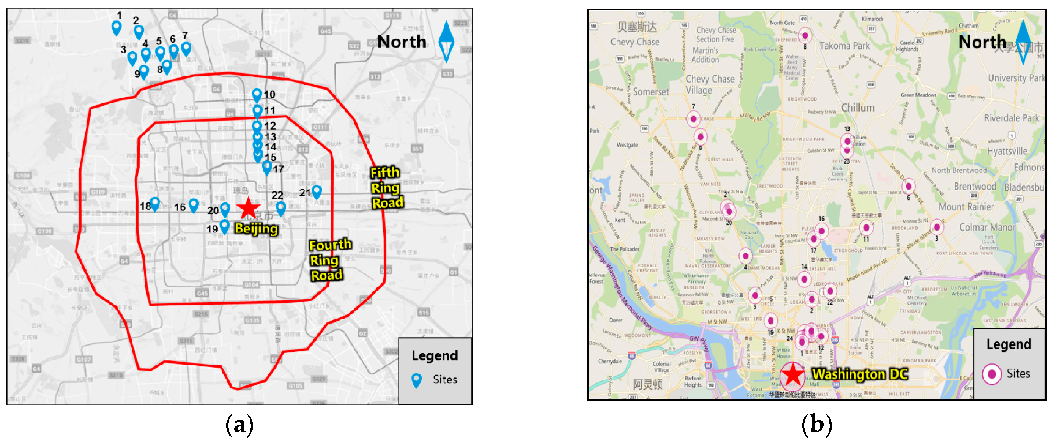
Figure 1 shows the research framework of this study. Firstly, the collection data were composed of two parts. One is from Beijing. The other one is from Washington, DC. Secondly, there is a comparison of observed saturation flow rates and estimation values from conventional method. The Chinese National Standard (Standard number is GB50647, Standard name is code for planning of intersections on urban roads) adjustment factor values and formula for calculating saturation flow rate were used with Beijing data. The Washington, DC data were used for estimating saturation flow rate with Highway Capacity Manual (HCM) adjustment factor values. Thirdly, the interaction between adjustment factors was verified using two-way analysis of variance (ANOVA). The two-way ANOVA is a common technology that is used for verifying the interactions. Finally, a new model considering the interaction between two factors was proposed by multiple linear regression method.

3.2. Study Site

To analyze the relationship between lane width and percentage of heavy vehicles, 35 through lanes at 22 intersections located in Beijing were included in this study (as shown in Figure 2a). At the same time, to verify the interaction between lane width and the proportion of left-turning vehicles, 25 shared left-turn lanes at 24 intersections (as shown in Figure 2b) were used for this research in Washington, DC. Intersections without a left-turn protected-permitted signal phase or high opposing traffic for the left-turn movement of the study approach were not included. The data was extracted from a master’s thesis of Howard University (Olaoluwa Dairo, 2014).

In Beijing, data collection was conducted midweek (Tuesday, Wednesday, and Thursday) during the peak hours (morning: 07:00–09:00, afternoon: 16:30–19:00). In Washington, DC, data were collected on weekdays during the peak hours (morning: 07:00 and 09:30, midday: 12:00 and 14:30, afternoon peak: 16:00 and 18:30). Eight or more vehicles in the line were needed to follow the Highway Capacity Manual (HCM) method. All of the intersections were affected only by lane width and heavy vehicle factors and other factors were ideal.

Table 1. Study site characteristics in Beijing.

NO.	Intersection Name	Surveyed Approach	Subject Lane	Lane Width (m)
1	Yongfeng Rd. and Xibeiwang Rd.	SB	2 TH	3.30
		NB	1 TH	3.30
2	Houchangcun Rd. and Tangjialing Rd.	EB	1 TH	3.30
3	Mlianwabei Rd. and Zhuyuanzhong St.	WB	1 TH	4.00
4	Mlianwabei Rd. and Dongbeiwangxi Rd.	WB	1 TH	3.60
		EB	1 TH	3.30
5	Mlianwabei Rd. and Dongbeiwang Rd.	EB	1 TH	4.00
		WB	1 TH	3.60
6	Mlianwabei Rd. and Xianghuangqidong Rd.	EB	2 TH	3.60
		WB	2 TH	3.60
7	Shangdidong Rd. and Shangdi 3rd St.	EB	2 TH	3.60
8	Nongdanan Rd. andShucun Rd.	WB	1 TH	3.00
		EB	1 TH	3.30
9	China Agricultural University South Gate	EB	2 TH	3.30
		WB	1 TH	3.00
10	Anli Rd. and Waiguanxie St.	SB	1 TH	3.00
11	Anli Rd. and Huizhongbei Rd.	SB	1 TH	3.00
12	Anli Rd. and Anyuan Rd.	SB	1 TH	3.30
13	Anli Rd. and Hepinglibei St.	SB	1 TH	3.30
14	Anli Rd. and Datun Rd.	SB	1 TH	3.00
15	Anli Rd. and Huizhong Rd.	SB	1 TH	3.60
16	Baiyun Rd. and Sanlihedong Rd.	WB	1 TH	3.30
17	Dongzhimennei St. and Yonghegong St.	EB	2 TH	2.50
18	Xicui Rd. and Fuxing Rd.	WB	2 TH	2.70
19	Nanheng St. and Caishikou St.	EB	1 TH	3.60
20	Changchun St. and Xuanwummenxi St.	WB	1 TH	3.00
21	Jintai Rd. and Chaoyangbei Rd.	EB	1 TH	3.00
22	Beiijngzhan St. and Jianguomennei St.	EB	1 TH	3.30

Note: TH = Exclusive through lane; SB = Southbound; EB = Eastbound; WB = Westbound; NB = Northbound.

and

Table 2. Study site characteristics in Washington, DC.

NO.	Intersection Name	Surveyed Approach	Subject Lane	Lane Width (ft)
1	12th Street and H Street NW	WB	1 TH–LT	10.4
2	9th Street and Rhode Island Avenue NW	NB	1 TH–LT	10.5
3	Rhode Island Avenue	SB	1 TH–LT	10
4	Connecticut Avenue and Calvert Street NW	SB	1 TH–LT	9.7
5	R street and Florida Avenue NW	SB	1 TH–LT	11.5
6	South Dakota Avenue and Michigan Avenue NE	EB	1 TH–LT	11.1
7	Connecticut Avenue and Military Road	SB	1 TH–LT	9.5
8	Eastern Avenue and Georgia Avenue NW	NB	1 TH–LT	10.3
9	Connecticut Avenue and Nebraska Avenue NW	NB	1 TH–LT	9.8
10	9th Street and Mt Vernon Place NW	NB	1 TH–LT	10.1
11	Harewood Road and Michigan Avenue	SB	1 TH–LT	9.7
12	6th Street and Massachusetts Avenue NW	WB	1 TH–LT	13.6
13	Riggs Road and Rock Creek Church RD NE	EB	1 TH–LT	10.8
14	11th Street and U street NW	WB	1 TH–LT	9.7
15	9th street and New York Avenue NW	WB	1 TH–LT	12.5
16	Warder Street and Kenyon Street NW	SB	1 TH–LT	11.4
17	Columbia Avenue and Georgia Avenue	EB	1 TH–LT	11
18	11th Street and K street NW	NB	1 TH–LT	13.5
19	Connecticut Avenue and Rhode Island Avenue	WB	1 TH–LT	9.6
20	Connecticut Avenue and Ordway Street NW	NB	1 TH–LT	12.1
21	Connecticut Avenue and Porter Street	WB	1 TH–LT	11
22	Florida Avenue and 4th Street NE	WB	1 TH–LT	11.9
23	North Capitol and Gallatin Street	SB	1 TH–LT	9.1
24	12th Street and New York Avenue NW	WB	1 TH–LT	11.2
		SB	1 TH–LT	10.5

Note: TH–LT = Shared left-turn and through lane; SB = Southbound; EB = Eastbound; WB = Westbound; NB = Northbound.

present the list of intersections and their lane characteristics. The conditions were as follows:

⮚

Intersection approach grades were level;

⮚

No curb parking on the approaches;

⮚

No bus stop near the approaches;

⮚

The intersection approaches surveyed were on four-lane (or more) divided roadways to prevent the influence of the number of lanes in a lane group;

⮚

No pedestrian or bicycle activity during the green phase on the surveyed approach

⮚

Intersections were located in urban areas outside of Central Business District (CBD).

3.3. Collection Method

The data collection equipment consisted of a video camera (Sony, HDR-CX680, mounted on a tripod), a range finder (deli, DL9712), a stopwatch, and a data collection sheet used to record lane width and cycle-by-cycle queuing and incident data. Data were collected for through lane group on each approach. A video camera was used to collect the actual SFRs and the proportion of heavy vehicles. A range finder was used to collect the lane width data. The equipment was set up at least 15 min before recording time, and observers and the video camera operator synchronized their stopwatches. The video camera was installed on the high buildings or a pedestrian skyway near the approaches. The shooting angle was adjusted to cover the line-up area and clearly identify the stop line. Each surveyed approach was videotaped to provide a visual record of the elapsed time for each lane surveyed. In some intersections, the camera was placed near the departure legs facing the measured approaches; this is because there were no high buildings or pedestrian skyways near the intersections. The video camera was adjusted to the highest position on the tripod and it recorded the line area clearly. The survey observer used a stopwatch to identify the beginning of the green signal phase on the study approach and also recorded the number of queued vehicles (by lane).

Saturation headways were measured beginning when the rear axle of the fourth queued vehicle crossed the stop line; the cumulative elapsed time was measured when the rear axle of the last queued vehicle (which was stopped at the onset of the green phase) crossed the stop bar. Any impedance that could influence the saturation flow rate during a surveyed signal green phase was noted. The number of heavy vehicles was for each cycle. Figure 3 was shown by the measurement method.

The data were collected at each intersection approach: (1) the configuration of the approach lane, (2) the lane width of the through lane, (3) location of the through lanes in the approach, (4) land use, and (5) the number of heavy vehicles in each signal cycle. The outermost through lanes were the main sites for data collection because, according to the actual observation, passenger cars preferred to move on the inside through lanes. In contrast, heavy vehicles preferred to move on the outside through lanes. Therefore, the outermost through lanes were selected as much as possible to obtain more saturation headway in high proportions of heavy vehicles. The saturation flow rates were collected for at least 15 signal cycles per lane for 3.0, 3.3, and 3.6m lanes (with 29 lanes), and at least 70 cycles per lane for 2.5, 2.7, 4.0m lanes (with 6 lanes). The distribution of the SFR was uniform for each level of proportions of heavy vehicles.

3.4. Data Reduction

The saturation headway was extracted manually from the video. The videos were coded by intersection number and were played in KMPlayer (a media player, from Pandora TV, Korean). The time error was 0.001 s. First, the time when the rear axle of the 4th vehicle crossed the stop line at the beginning of the green phase was recorded. Second, the time when the last vehicle in the line crossed the stop line of the green phase was recorded. The total number of vehicles in the line was recorded. Finally, the sum time was divided by the number of headways after the fourth vehicle to obtain the average headway. The SFR was 3600 divided by this average headway. Bonneson [33] conducted a study where the headway was stable after the 4th vehicle, and the minimum headway did not occur before the 8th vehicle. Therefore, to measure the maximum saturation flow rate (SFR), it is necessary to measure the line of vehicles beyond the 10th vehicle. During the measurement, cycles with congestion or high volume of pedestrians and bicycles were not recorded. The number of heavy vehicles was recorded for each cycle. Average headway would be computed using the following Equation (1). The headway data were presented in the form shown in

Table 3. Saturation flow rate data study worksheet.

Intersection: Anli Rd. and Datun Rd. (Southbound)
Data: 2017-07-11		Lane width: 3.00 m			Location: middle
Time: 16:30~19:00
Cycle	T4 (s) 1	Tn (s) 2	N3	Number of Heavy Vehicles	The Percentage of Heavy Vehicles	Average Headway (s)
1	10.84	25.67	10	0	0%	2.47
2	11.1	27.3	12	1	8.33%	2.03
3	16.33	33.59	10	2	20%	2.88
4	11.92	23.46	10	0	0%	1.92
5	16.22	36.49	10	3	30%	3.38
6	13.69	31.35	11	1	9.09%	2.52
7	13.04	35.99	14	0	0%	2.30
……	……	……		……	……	……
20	10.16	20.29	10	3	30%	3.36

¹ T₄ is time when the rear axle of the 4th vehicle on the green phase crossed the stop line (sec). ² T_n is time when the rear axle of the last vehicle on the green phase crossed the stop line (sec). ³ N is number of vehicles line up on the green phase.

.

$$h=\frac{(T_n-T_4)}{(N-4)},$$

(2)

where, T_n is time when the rear axle of the last vehicle on the green phase crossed the stop line (sec), T₄ is time when the rear axle of the 4th vehicle on the green phase crossed the stop line (sec), and N is number of vehicles line up on the green phase.

4. Results and Discussion

4.1. Data Summary

Lane width and the percentage of heavy vehicles. The lane width distribution was based on the common lane width in Beijing: 2.5 m (2.7, 3.0, 3.25, 3.5, and 4.0 m). The distribution of the proportion of heavy vehicles ranged from 0% to 50%. In total, 876 average headway samples (cycles) were recorded from 35 through lanes. The maximum was 4.60 s. The minimum was 1.99 s. To discover the data features, the average headways were sorted according to the lane width and the percentage of heavy vehicles, from small to large (as shown in Figure 4). Obviously, a significant association between saturation headway and percentage of heavy vehicles was observed. The saturation headway increased with the increase of percentage of heavy vehicles. However, the difference between lane widths was not significant.

Lane width and the proportion of left-turning vehicles. There are 25 types of lane widths in this research: 8.5, 9, 9.1, 9.4, 9.5, 9.6, 9.7, 9.8, 9.9, 10, 10.1, 10.4, 10.5, 10.8, 11, 11.1, 11.2, 11.4, 11.5, 11.9, 12.1, 12.5, 13.1, 13.5, and 13.6 ft. To simplify the analysis, the types of lane widths fall into three categories based on the Highway Capacity Manual (HCM): <10, 10–12.9, and ≥13 ft. The distribution of the proportion of left-turning vehicles ranged from 0% to 100%. In total, 521 average headway samples (cycles) were recorded at 25 through lanes. The maximum was 5.50 s. The minimum was 1.50 s. Similarly, the average headways were sorted according to the lane width and the proportion of left-turning vehicles from small to large (as shown in Figure 5). The relationship between saturation headway and left-turn proportion was not obvious. For the detailed analysis, observed saturation headway showed an increased tendency as the left-turn proportion increased.

4.2. Satruation Flow Rate Field Observation versus Conventional Method

In the last section, we observed the measured data and analyzed the relationship between saturation headway and adjustment factors. For further analysis, this section compares the difference between the current saturation flow rate (SFR) adjustment model and SFR field observations. The following statistic was employed: the mean absolute percentage error (MAPE), which is defined as follows:

$$MAPE=\frac{1}{N}\left|\frac{s_p-s_{adj}}{s_p}\right|,$$

(3)

where S_adj is adjusted SFR by Highway Capacity Manual (HCM) or Chinese National Standard GB50647, and S_p is observed SFR.

Since the first edition of the Highway Capacity Manual (HCM) was published in 1950, the HCM was updated five times. All world countries have also developed highway capacity manuals based on their local traffic characteristics. They follow the method of US HCM. China is no exception, and the Chinese National Standard GB50647 (Code for Planning of Intersections on Urban Roads) has been established [19]. The saturation flow rate (SFR) model of GB50647 is similar to the HCM model and is a multiplication model. However, the parameters of the GB50647 model are adjusted according to local traffic characteristics, mainly reflected in two aspects: (1) based saturation flow rate (BSFR) (the classification was more detailed, different default values were given by region and lane type), and (2) adjustment factors (the lane width values in code are common lane types in China). The factor of percentage of heavy vehicles is based on the Canadian Capacity Guide for Signalized Intersections [16], shown in

Table 4. Factors in Highway Capacity Manual (HCM) versus Chinese National Standard GB50647.

Factors	HCM 1	GB50647 2
BSFR	Metro pop ≥ 250,000: 1900 pcu/h/ln Otherwise: 1750 pch/h/ln	Eastern cities: 1750 pcu/h/ln Central cities: 1650 pcu/h/ln Western cities: 1550 pcu/h/ln
Lane Width	<10.0 ft (3.05 m) 0.96 10.0–12.9 ft (3.9 m) 1.00 >12.9 ft (3.9 m) 1.04	2.70 m: 0.88 2.80 m: 0.92 2.90 m: 0.96 3.00 m: 1.00 3.25 m: 1.08 3.50 m: 1.14 3.75 m: 1.17 4.00 m: 1.18
Percent Heavy Vehicles	$f_{HVg}=\frac{100-0.78·P_{HV}}{100}$	$f_g=1-\left(G+HV\right)$
Left Turn	$s_{lr}=\frac{s_{th}}{1+P{}_L\left(E_L-1\right)}$	-

¹ HCM is the acronym of Highway Capacity Manual. ² GB50647 is the standard number of Chinese National Standard.

.

First, the data in Washington, DC were analyzed by the parameters in Highway Capacity Manual (HCM). Second, the data in Beijing were analyzed by the parameters of Chinese National Standard GB50647. Finally, the model of saturation flow rate is compared with the observation, and the results are shown in Figure 6 and Figure 7. Most of the mean absolute percentage error (MAPE) of the 25 shared through and left-turn lanes using the HCM method were more than 20%. The MAPE of all of this data was 33.16%. Most of the MAPE of the 35 through lanes with Chinese National Standard GB50647 method was more than 10%. The MAPE of all of this data was 13.64%.

The diagrams of two adjustment factors and saturation headways are shown. Comparing the saturation headway adjustment model and the saturation headway field observation, we can find the reason for the errors. As shown in Figure 8, there is a difference between the model values and observed values. In the model data, the saturation headway increased evenly with increasing percentage of heavy vehicles (PoHV) in each width lane. However, in the measured data, the change of saturation headway with increasing percentage of heavy vehicles was significant, and the same is found for the model data in “narrow” lanes (area A). The change of saturation headway with increasing percentage of heavy vehicles was not significant in “wide” lanes (area B). As shown in Figure 9, on the one hand, the measured saturation headways were larger than the model values, indicating that the base saturation flow rate (BSFR) was not adjusted. On the other hand, left-turning vehicles had a great impact on saturation flow rates. In addition, there was an interaction between lane width (LW) and proportion of left-turning vehicles (PoLV). Above all, there were two reasons why the errors were large: (1) because the BSFR was not adjusted according to the local data and thus adopted the default value of Highway Capacity Manual (HCM) and Chinese National Standard GB50647, and (2) the interactional relationship between lane width and percentage of heavy vehicles was not deeply considered. Similarly, the interaction between lane width and proportion of left-turning vehicles was ignored.

4.3. Interaction between Adjustment Factors Verifications

To verify the interaction between the factors, the common method is two-way analysis of variance (ANOVA). In this research, the lane width (LW) factor is a discrete variable. The percentage of heavy vehicles (PoHV) factor and proportion of left-turning vehicles (PoLV) factor are continuous variables. According to Beijing data, there are six types of LW, which can be directly classified into six categories. The PoHV are divided into 0%, (0–10%), (10–20%), (20–30%), (30–40%), and (40–50%), i.e., six classes based on the Edwin E. Lewis [32] method. According to the Washington, DC, data, there are 25 types of LW, which can be directly classified into three categories by Highway Capacity Manual (HCM). They are <10 ft., 10.0–12.9 ft., and ≥13 ft., respectively. The PoLV are divided into 0%, (0–10%), (10–20%), (20–30%), (30–40%), (40–50%), (50–100%), and 100%, i.e., eight classes. Then, a two-way ANOVA was used to evaluate the effects of the interactions between LW and PoHV, PoLV on the saturation flow rate (SFR), at a 5% level of significance. The two-way ANOVA summaries are shown in

Table 5. Summary of two-way ANOVA with LW and PoHV.

	Type III Sum of Squares	df 1	Mean Square	F 2	Sig. 3
Corrected Model	232.520a	35	6.643	274.735	0.000
Intercept	4998.605	1	6209.833	256803.731	0.000
LW	37.433	5	7.487	309.602	0.000
PoHV	174.237	5	34.847	1441.092	0.000
LW*PoHV	17.394	25	0.696	28.773	0.000
Error	20.312	840	0.024
Total	6972.074	876
Corrected Total	252.832	875

¹ df means degree of freedom. ² F means F-test statistic value. ³ Sig. means p-value and stands for significance level.

and

Table 6. Summary of two-way ANOVA with LW and PoLV.

	Type III Sum of Squares	df 1	Mean Square	F 2	Sig. 3
Corrected Model	49.564a	21	2.360	7.763	0.000
Intercept	933.989	1	933.989	3071.966	0.000
LW	23.851	7	3.407	11.207	0.000
PoLV	9.269	2	4.635	15.244	0.000
LW*PoLV	8.011	12	0.668	2.196	0.011
Error	151.714	499	0.304
Total	4032.380	521
Corrected Total	201.279	520

¹ df means degree of freedom. ² F means F-test statistic value. ³ Sig. means p-value and stands for significance level.

.

As shown in Table 3, the null hypothesis (LW) which was that there was no relationship between SFRs and different lane widths, was rejected (p = 0.000 < 0.05). There was a difference of SFR among the various lane widths. The null hypothesis (PoHV), which was that there was no relationship between SFRs and different percent heavy vehicles, was rejected (p = 0.000 < 0.05). There was a difference of SFR among various percents of heavy vehicles. The p-value of F (LW*PoHV) was also less than 0.05. The null hypothesis (LW*PoHV) was thus rejected. It appeared likely that there was a significant interaction between lane width and heavy vehicles affecting saturation headway. In other words, under different lane width factors, the effect on saturation flow rate varied for each level of the percentage of heavy vehicles. Similarly, in Table 4, the p-values of F (LW, PoLV, LW*PoLV) were less than 0.05. The null hypotheses (LW, PoLV, LW*PoLV) were thus rejected. It appeared likely that there was also a significant interaction between lane width and left-turning vehicles affecting saturation headway.

4.4. Saturation Flow Rate Model Considering the Intersection

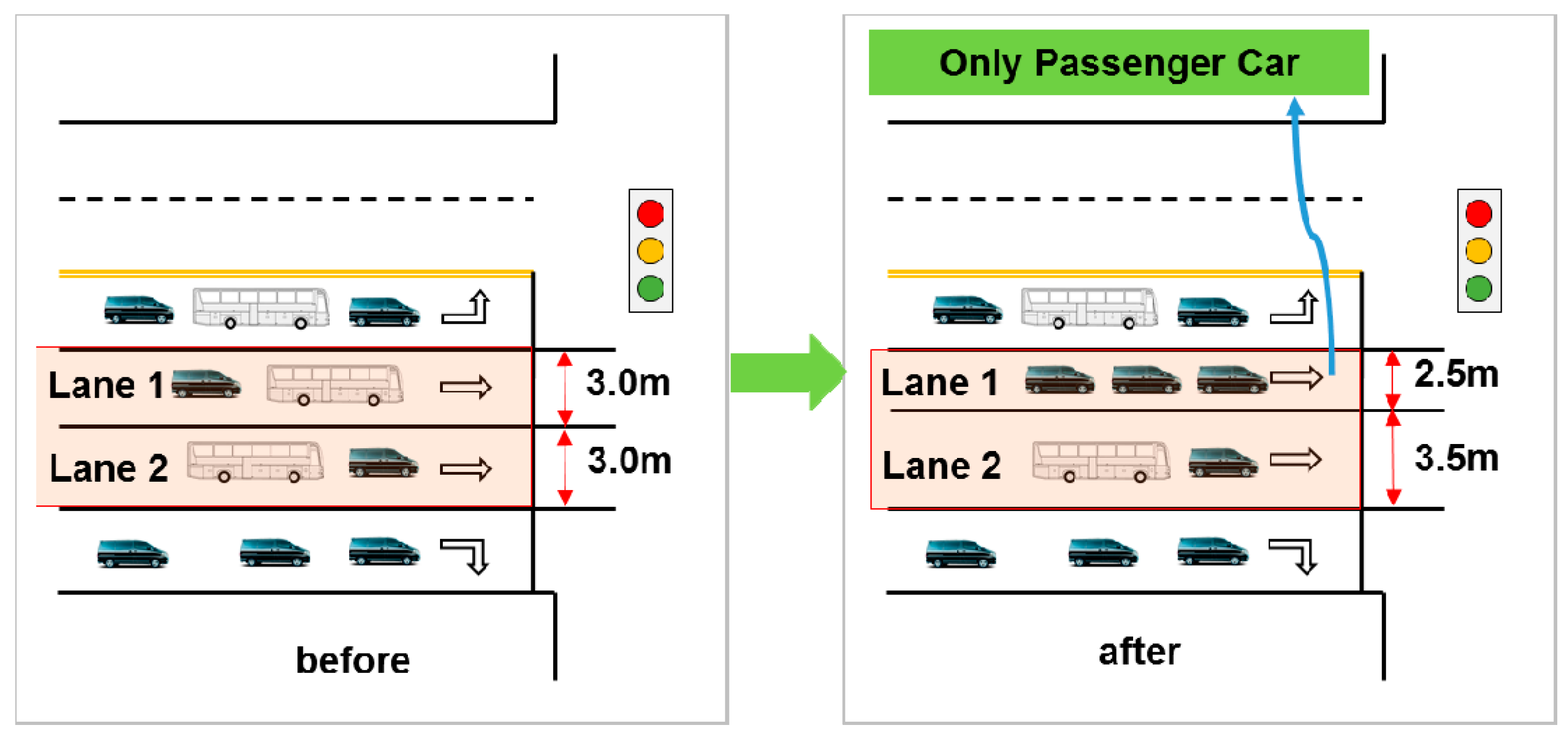
From the above, it can be seen that there were interactions between lane width (LW) and percentage of heavy vehicles (PoHV) and proportion of left-turning vehicles (PoLV). However, the factors affecting the saturation flow rate (SFR) were independent. Therefore, the larger errors of saturation flow rate estimated would still occur when engineers used the current SFR model. By using the multiple linear regression (MLR) method, we constructed a comprehensive adjustment factor model considering the interactions. The prediction ability of the saturation flow rate model would be improved. First, the linear relationship between saturation headway and the adjustment factors was established. Multiplication of the two factors as an interaction term was introduced into the model. Since the adjustment factors in the Beijing and Washington data were different, two models needed to be built. The results are shown in

Table 7. Summary of multiple linear regression.

Model		Unstandardized Coefficients		t 3	Sig. 4
		B 1	Std. Error 2
Model 1 with Beijing Data	Constant	2.690	0.065	41.570	0.000
	LW(1)	−0.131	0.020	−6.506	0.000
	PoHV	6.928	0.260	26.686	0.000
	LW*PoHV	−1.295	0.080	−16.246	0.000
Model 2 with Washington Data	Constant	2.861	0.306	9.346	0.000
	LW(2)	−0.032	0.029	−1.105	0.270
	PoLV	3.283	1.294	2.538	0.011
	LW*PoLV	−0.217	0.124	−1.743	0.082

¹ B means coefficient of regression. ² Std. Error means standard error mean which is the estimated standard deviation of the sample mean. ³ t means t-test statistic value. ⁴ Sig. means p-value and stands for significance level.

and

Table 8. Test statistics.

Model	R 1	R Square 2	Adjusted R Square 3	Std. Error of the Estimate 4
Model 1	0.939	0.881	0.881	0.186
Model 2	0.391	0.153	0.148	0.574

¹ R means multiple correlation coefficient. ² R Square means coefficient of determination. ³ Adjusted R Square means adjusted coefficient of determination. ⁴ Sig. means p-value and stands for significance level.

. Second, we used a reciprocal model S = 3600/h to find the biased saturation headway. Biased saturation headway that divided the model of the first step was a comprehensive adjustment factor model, as shown in Equations (3) and (4).

$$f_{c1}=\frac{2.18}{h_t}=\frac{2.18}{2.69-0.131·LW(1)+6.928·PoHV-1.295·LW(1)·PoHV}$$

(4)

$$f_{c2}=\frac{1.89}{h_t}=\frac{1.89}{2.861-0.032·LW(2)+3.283·PoLV-0.217·LW(2)·PoLV}$$

(5)

where f_c1 is comprehensive adjustment factor in Model 1, f_c2 is comprehensive adjustment factor in Model 2, LW(1) is lane width (m), LW(2) is lane width (ft.), PoHV is percentage of heavy vehicles (%), and PoLV is proportion of left-turning vehicles (%).

As shown in Table 7 and Table 8, there was a significant linear relationship between saturation headway and lane width (LW), percentage of heavy vehicles (PoHV), and LW*PoHV. The model had a high goodness of fit (R square is 0.881). The coefficient of LW was negative, indicating that the wider the lane, the smaller the saturation headway time. The coefficient of percentage of heavy vehicles was positive, indicating that the larger the percentage of heavy vehicles, the larger the saturation headway time. The p value of each coefficient was less than 0.05. All variables could be retained in the equation. However, the linear relationship between saturation headway and lane width (LW), proportion of left-turning vehicles (PoLV) and LW*PoLV was not significant. The model had a low goodness of fit (R square is 0.148), indicating that the relationship between the independent and dependent variables was complex and nonlinear. However, this paper was an exploratory study. This model could explain some information. Similarly, the coefficient of LW was negative. The coefficient of proportion of left-turning vehicles was positive. Above all, we found that all relationships between the saturation headway and each adjustment factor were not linear. There were complex interactions between the factors. If there were fewer factors, and the linear relationship between saturation headway and factor was significant, we could build the model by a statistical method to reveal interaction. In contrast, we should introduce a nonlinear model to analyze.

The saturation flow rates (SFR) are estimated and compared with the measured saturation flow rates. The mean absolute percentage error (MAPE) indicators are again used. The results are shown in Figure 10 and Figure 11. In Beijing, all errors in the 35 through lanes decreased with the new SFR model. The MAPE of all data was reduced to 4.89%, down from 13.64%. In Washington, DC, all errors in the 25 shared left-turn lanes decreased with the new SFR model. The MAPE of all data was reduced to 14.56%, down from 33.16%.

4.5. Application

Considering the complex interaction between adjustment factors, the estimation accuracy of saturation flow rate could be improved, and a new perspective can be provided for the current traffic operation. This improvement can help to better the signalized intersection capacity. For example, in the previous analysis, it was shown that there was an interaction between adjustment factor for lane width and adjustment factor for heavy vehicles in traffic stream. In the narrow lanes, the changes to saturation flow rate were significant with the changes of percentage of heavy vehicles. In the wide lanes, the changes to saturation flow rate were not significant. We can make some improvements in the multi-through-lane width design as follows.

For example, there is an assumptive approach which is composed of a left-turn lane, a right-turn lane and two through lanes in Beijing. All lanes are 3.0 m wide. The signal cycle length is 120 s. The percentage of heavy vehicles is 15% at two through lanes, respectively. Based on the current situation, we only change the through lanes width design and vehicles operation management rules. As is shown in Figure 12, lane 1 width was adjusted to 2.5 m and lane 2 width to 3.5 m. The width of through lane group has not changed and is still 6.0 m. After adjusting for the lane width, all the heavy vehicles should enter lane 2 (3.5 m). There are only passenger cars in lane 1 (2.5 m). The percentage of heavy vehicles has increased (30%) in lane 2. The percentage of heavy vehicles has dropped to 0% in lane 1. There was no change in percentage of heavy vehicles in through lane group (15%).

Two different methods of width design are tested to find the lane group capacity, vehicle delays, and emissions. The saturation flow rates are calculated by the proposed method. We calculate the delays with Highway Capacity Manual (HCM) method [10] which is shown in Equation (5). The emissions are calculated by the results of Zhao’s paper [5]. The CO₂, CO, HC, and NO_X emissions per vehicle during one cycle (cycle length is 120 s) is 136.51, 0.72, 0.06, and 0.09 g, respectively. The results are shown in

Table 9. Comparison of the performance indexes in the approach with different design methods.

	Original Design		Adjusted Design
Through Lane Group	Lane 1	Lane 2	Lane 1	Lane 2
Lane Width (m)	3.0	3.0	2.5	3.5
Base Saturation Flow Rate (pcu/h)	1650	1650	1650	1650
Proposed adjusted factor	0.792	0.792	0.923	0.838
Adjusted Saturation Flow Rate (veh/h)	1306	1306	1523	1382
Lane Group Adjusted Saturation Flow Rate (veh/h)	2612		2905
Average vehicle Delay (s)	24.3		22.8
Emissions Changes (g)	CO2: 40,000
	CO: 210.9
	HC: 17.58
	NOX: 26.37

. After adjusting for the lane width, the saturation flow rate of through lane group has increased by 293 veh/h (11.22%). The average per vehicle delay has an obvious decrease (6.18%). With new lane width design, the missions have an obvious reduction. There are 293 vehicles passing the stop line without waiting to pass through the intersection. All CO₂, CO, HC, and NOX emissions at one hour reduced by 40 kg and 210.9, 17.58, and 26.37 g, respectively. It is shown that simple design can improve traffic capacity and reduce delays and emissions.

$$d=\frac{0.5C{(1-g/C)}^2}{1-[\min (1,X)g/C]}$$

(6)

where, g is effective green time, C is cycle time, and X is volume-to-capacity ratio.

5. Conclusions

Lane width, percentage of heavy vehicles, and proportion of left-turning vehicles were the important factors affecting the saturation flow rate. In past studies, the relationship between each factor and SFR was considered independently. Based on measured data in Beijing and Washington, DC, this paper validated the interaction between factors. A new saturation flow rate estimation model that considers the interaction was also established. It was found that:

⮚

The adjustment factors were nonindependent. There was an interaction between them.

⮚

The influence of percentage of heavy vehicles on saturation flow rate was more obvious in narrow lanes than in wide lanes.

⮚

The influence of proportion of left-turning vehicles on saturation flow rate was more obvious in narrow lanes than in wide lanes.

⮚

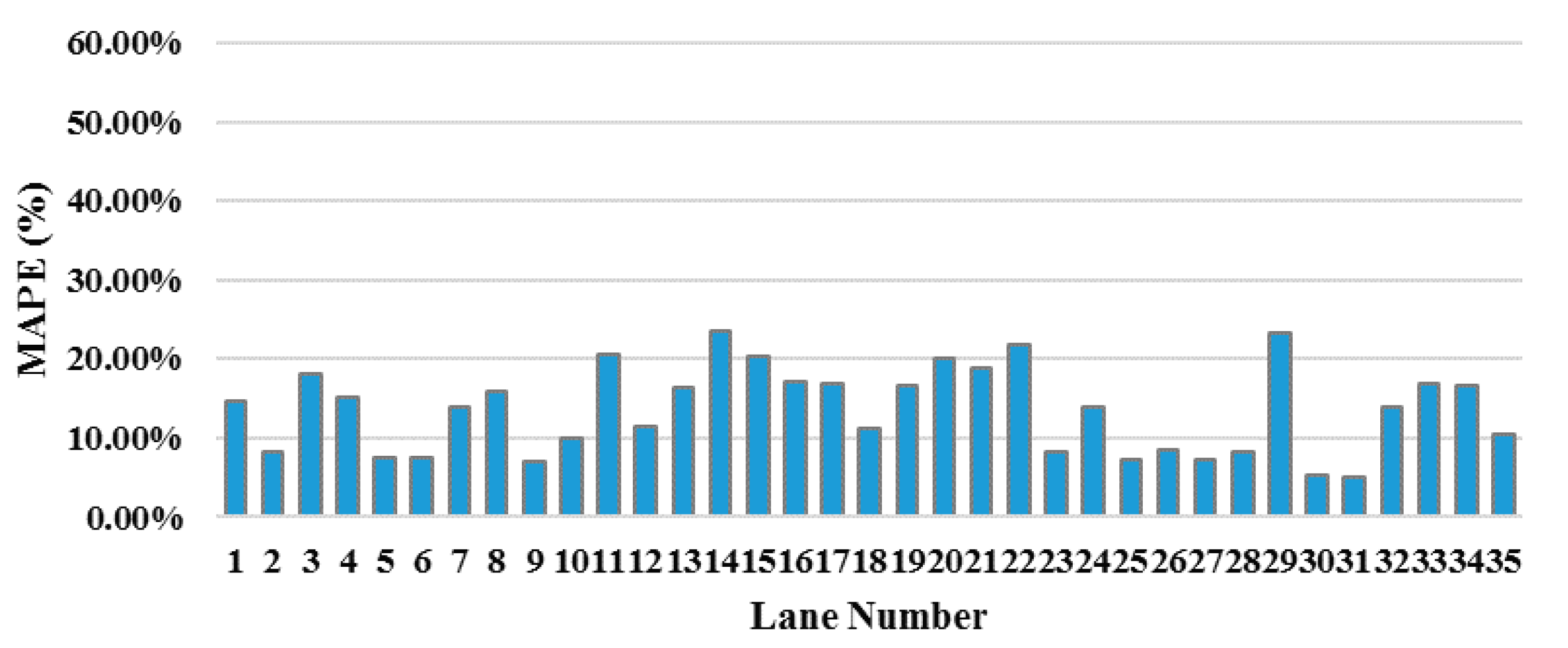
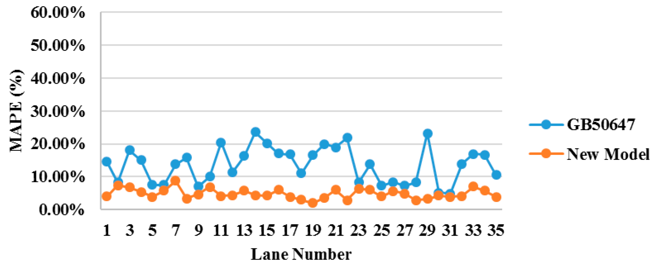
Two new comprehensive adjustment factor models were built by multiple linear regression (MLR) method. In Beijing, the mean absolute percentage error (MAPE) was reduced to 4.89% down from 13.64%. In Washington, DC, the MAPE was reduced to 14.56% down from 33.16%.

At the same time, the model provided support for Highway Capacity Manual (HCM) localization and could help Beijing and Washington, DC engineers to estimate the SFR more accurately. The level of designing and operation was improved. The traffic congestions and emissions were reduced. Due to the limitation of survey data, this paper is an exploratory research with certain limitations. In order to apply it to engineering projects, the data should be further expanded. In the future, this research will continue regarding two aspects. On the one hand, we will analyze whether there are interactions between other factors. On the other hand, the relationship between the adjustment factors will be restructured by data-driven methods.

References

1. Zhao, J.; Ma, W.; Xu, H. Increasing the Capacity of the Intersection Downstream of the Freeway Off-Ramp Using Presignals. Comput. Aided Civ. Infrastruct. Eng. 2017, 32, 674–690. [Google Scholar] [CrossRef]
2. Beijing Transport Institute. 2019 Beijing Transport Annual Report; Beijing Transport Institute: Beijing, China, 2019; pp. 1–2. [Google Scholar]
3. Xia, X.; Ma, X.; Wang, J. Control Method for Signalized Intersection with Integrated Waiting Area. Appl. Sci. 2019, 9, 968. [Google Scholar] [CrossRef] [Green Version]
4. Li, X.; Li, G.; Pang, S.S.; Yang, X.; Tian, J. Signal timing of intersections using integrated optimization of traffic quality, emissions and fuel consumption: A note. Transp. Res. D Transp. Environ. 2004, 9, 401–407. [Google Scholar] [CrossRef]
5. Zhao, H.; He, R.; Jia, X. Estimation and Analysis of Vehicle Exhaust Emissions at Signalized Intersections Using a Car-Following Model. Sustainability 2019, 11, 3992. [Google Scholar] [CrossRef] [Green Version]
6. Zhao, J.; Liu, Y.; Wang, T. Increasing signalized intersection capacity with unconventional use of special width approach lanes. Comput. Aided Civ. Infrastruct. Eng. 2016, 31, 794–810. [Google Scholar] [CrossRef]
7. Qin, Z.; Zhao, J.; Liang, S.; Yao, J. Impact of Guideline Markings on Saturation Flow Rate at Signalized Intersections. J. Adv. Transp. 2019, 2019, 1–14. [Google Scholar] [CrossRef]
8. Xuan, Y.; Carlos, F.D.; Michael, J.C. Increasing the capacity of signalized intersections with separate left turn phases. Transp. Res. B Methodol. 2011, 45, 769–781. [Google Scholar] [CrossRef]
9. Yan, C.; Jiang, H.; Xie, S. Capacity optimization of an isolated intersection under the phase swap sorting strategy. Transp. Res. B Methodol. 2014, 60, 85–106. [Google Scholar] [CrossRef]
10. Transportation Research Board. Highway Capacity Manual; National Research Council: Washington, DC, USA, 2010; p. 34. ISBN 978-0-309-16077-3. [Google Scholar]
11. Shao, C.; Liu, X. Estimation of saturation flow rates at signalized intersections. Discret. Dyn. Nat. Soc. 2012, 2012, 1–10. [Google Scholar] [CrossRef]
12. TRRL (Transport and Road Research Laboratory). The Prediction of Saturation Fows for Road Junctions Controlled by Traffic Signals; TRRL: Wokingham, UK, 1986; p. 3. ISBN 0266-5247. [Google Scholar]
13. ARRB (The Australian Road Research Board). Traffic Signals: Capacity and Timing Analysis; ARRB: Melbourne, Victoria, Australia, 1981; p. 1. ISBN 1445-4467. [Google Scholar]
14. Tarko, A.P.; Marian, T. Uncertainty in saturation flow predictions. Red 2000, 1, 2. [Google Scholar]
15. Transportation Research Board. Highway Capacity Manual; National Research Council: Washington, DC, USA, 2016; p. 34. ISBN 978-0-309-37000-4. [Google Scholar]
16. Committee on the Canadian Capacity Guide for Signalized Intersections. Canadian Capacity Guide for Signalized Intersections; Institute of Transportation Engineers: Washington, DC, USA, 2008; pp. 42–68, ISBN-10 1-933452-24-2. [Google Scholar]
17. Forschungsgesellschaft für Straßen- und Verkehrswesen (FGSV). Handbuch für die Bemessung von Straßenverkehrsanlagen (HBS); FGSV: Köln, Germany, 2015; pp. 80–90. ISBN 978-3-86446-103-3. [Google Scholar]
18. Council of Scientific and Industrial Research (CSIR). Indian Highway Capacity Manual (Indo-HCM); CSIR: New Delhi, India, 2017; p. 39. [Google Scholar]
19. Tongji University. Code for Planning of Intersections on Urban Roads (GB50647-2011); China Planning Press: Beijing, China, 2011; p. 77. [Google Scholar]
20. Zegeer, J.D. Field validation of intersection capacity factors. Transp. Res. Rec. 1986, 1901, 67–68. [Google Scholar]
21. Potts, I.B.; Ringert, J.F.; Bauer, K.M.; Zegeer, J.D.; Harwood, D.W.; Gilmore, D.K. Relationship of lane width to saturation flow rate on urban and suburban signalized intersection approaches. Transp. Res. Rec. 2007, 2027, 45–51. [Google Scholar] [CrossRef]
22. Hung, W.T.; Tian, F.; Tong, H.Y. Discharge headway at signalized intersections in Hong Kong. J. Adv. Transp. 2003, 37, 105–117. [Google Scholar] [CrossRef]
23. Radhakrishnan, P.; Tom, V. Mathew. Passenger car units and saturation flow models for highly heterogeneous traffic at urban signalized intersections. Transportmetrica 2011, 7, 141–162. [Google Scholar] [CrossRef]
24. Biswas, S.; Chakraborty, S.; Ghosh, I.; Chandra, S. Saturation flow model for signalized intersection under mixed traffic condition. Transp. Res. Rec. 2018, 2672, 55–65. [Google Scholar] [CrossRef]
25. Kimber, R.M.; McDonald, M.; Hounsell, N. Passenger car units in saturation flows: Concept, definition, derivation. Transp. Res. B Methodol. 1985, 19, 39–61. [Google Scholar] [CrossRef]
26. Venkatesan, K.; Asaithambi, G.; Sivanandan, R. Development of microscopic simulation model for heterogeneous traffic using object oriented approach. Transportmetrica 2008, 4, 227–247. [Google Scholar] [CrossRef]
27. Levinson, H.S. Capacity of Shared Left-turn Lanes-A Simplified Approach. Transp. Res. Rec. 1989, 1225, 45–47. [Google Scholar]
28. Chen, P.; Qi, H.; Sun, J. Investigation of saturation flow on shared right-turn lane at signalized intersections. Transp. Res. Rec. 2014, 2461, 66–75. [Google Scholar] [CrossRef]
29. Lin, F. Saturation flow and capacity of shared permissive left-turn lane. J. Transp. Eng. 1992, 118, 611–630. [Google Scholar] [CrossRef]
30. Zhou, Y.; Zhuang, H. Traffic performance in signalized intersection with shared lane and left-turn waiting area established. J. Transp. Eng. 2011, 138, 852–862. [Google Scholar] [CrossRef]
31. Tsao, S.; Chu, S. Adjustment factors for heavy vehicles at signalized intersections. J. Transp. Eng. 1995, 121, 150–157. [Google Scholar] [CrossRef]
32. Lewis, E.E.; Rahim, F.B. Saturation flow rate study at signalized intersections in Panama. In Proceedings of the 86th Annual Meeting of the Transportation Research Board, Washington, DC, USA, 21–25 January 2007. [Google Scholar]
33. Bonneson, J.A. Modeling Queued Driver Behavior at Signalized Junctions. Transp. Res. Rec. 1992, 1, 99. [Google Scholar]
Figure 1. Research framework.
Sustainability 12 00665 g001
Figure 2. Location of selected sites: (a) Location of selected sites in Beijing; (b) Location of selected sites in Washington, DC.
Sustainability 12 00665 g002
Figure 3. Placement of video cameras at intersections in Beijing: (a) Cameras were placed on high buildings; (b) Cameras were placed on departure.
Sustainability 12 00665 g003
Figure 4. Distribution of field saturation headway by lane width and percentage of heavy vehicles.
Sustainability 12 00665 g004
Figure 5. Distribution of field saturation headway by lane width and proportion of left-turning vehicles.
Sustainability 12 00665 g005
Figure 6. Mean absolute percentage error (MAPE) of calculation values in Beijing: adjustment factors are lane width and percentage of heavy vehicles.
Sustainability 12 00665 g006
Figure 7. MAPE of calculation values in Washington, DC: adjustment factors are lane width and proportion of left-turning vehicles.
Sustainability 12 00665 g007
Figure 8. The effects of lane width (LW) and percentage of heavy vehicles (PoHV) on saturation headway with Beijing Data: (a) The relationship of LW, PoHV, and saturation headways by observation; (b) The relationship of LW, PoHV, and saturation headways by Chinese National Standard GB50647.
Sustainability 12 00665 g008
Figure 9. The effects of lane width (LW) and proportion of left-turning vehicles (PoLV) on saturation headway with Washington, DC, Data: (a) The relationship of LW, PoLV, and saturation headways by observation; (b) The relationship of LW, PoLV, and saturation headways by HCM.
Sustainability 12 00665 g009
Figure 10. Mean absolute percentage error (MAPE) of estimated saturation flow rate (SFR) by New Model versus Chinese National Standard GB50647 factors.
Sustainability 12 00665 g010
Figure 11. Mean absolute percentage error (MAPE) of estimated saturation flow rate (SFR) by new model versus HCM factors.
Sustainability 12 00665 g011
Figure 12. The improvements of the multi-through-lane width design.
Sustainability 12 00665 g012