Accessibility, Infrastructure Provision and Residential Land Value: Modelling the Relation Using Geographic Weighted Regression in the City of Rajkot, India

Abstract

Amenities and infrastructure provision in urban areas are essential for the sustainable future of cities in developing countries like India. Indian cities have large development deficits and find it challenging to bridge the gap using traditional methods. Provision of these facilities costs money, which is often not available. However, access to amenities and infrastructure adds to land premium, which, if captured, can be used to finance the provision of these facilities. In India, very little information is available on the value of accessibility and infrastructure provision, and thus, these indirect benefits are primarily ignored by urban planners. This study fills the gap by identifying these benefits using Rajkot city in India as a case study. A geographic weighted regression model is used to model the relationship. It is found that land price variation is explained to a good extent using the model. Estimates show that infrastructure and amenities have a substantial impact on land value, much higher than the cost required to provide these.

1. Introduction

The future of cities in India will depend upon how well they can bridge development deficits of inadequate and insufficient infrastructure provision [1]. This deficit is enormous, with an annual estimate of the investment required at around USD 45,000 Million [2,3]. Traditional infrastructure funding methods have not worked effectively, and therefore, the government of India is considering options to finance urban infrastructure using alternatives like the land value capture mechanism [2]. The premise is that land value increases with the provision of infrastructure and can be used to fund the infrastructure costs [4]. However, to date, very few studies in India have looked at the impact of infrastructure and other amenities on land value [5]. Thus, there is a gap in the literature, which needs to be filled.

The relations are studied using the city of Rajkot, a typical medium-sized Indian city located in the state of Gujarat in western India, as a case city. The purpose is to contribute to the existing literature by considering and analysing the spatial distribution and effects of accessibility and infrastructure provision on the land value used for residential purposes.

This paper is divided further into five sections. The next section is a review of literature, which is followed by a description of the case area and discussion on methods and data handling. The fifth section is a presentation of results followed by the conclusion.

2. Literature Review

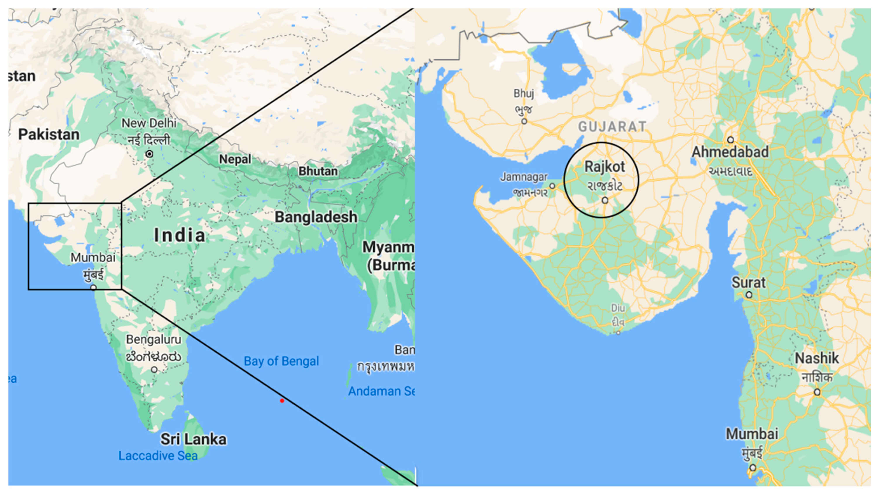
Accessibility and land value are closely related. The location of the land/property, the location of surrounding facilities, and the available transport infrastructure determine accessibility to desired activities [6,7]. Property values around locations with higher accessibility often come with a higher premium. Therefore, accessibility to jobs and land value has gotten much attention in the land-market studies starting with the model proposed by Alonso [8], which suggested that land prices fall with an increase in distance from the city centre. Cities like Rajkot are spatially dispersed and have secondary employment centres in addition to the traditional city core, which can also impact the accessibility to activities [9,10,11]. Job accessibility is a function of both population (demand), jobs (supply), and transport (distance between demand and supply); gravity-based measures are used to explain the property prices [7,12]. There is a large body of literature on the impact of accessibility on residential properties. Nelson [13] found that for every kilometre away from the city centre mean distance the property prices increased by USD 23/m². Dziauddin et al. [14] found that nearness (in metres) to the central business district (CBD) increases the property value by 0.21%, Ding et al. [15] found that a 10% increase in accessibility (job proximity indexed between 1 and 10) increases the property value by 4.5%. A 1% increase in accessibility to sub-centres results in up to 2.2% increase in property prices in Mexico City [16].

Proximity and thereby access to public transport characterises connectivity to a more extensive transit network and is therefore used to explain the rise in property prices. The bus rapid transit system was found to have a positive impact on property prices, for example, 13% and 14% in Bogota [17], 11%–13% [18], 5%–10% in Seoul [19]. Welch et al. [20] observed that with every one metre of distance from the nearest rail station, the property prices were reduced by USD 1.54., proximity to the metro increased property values by 6.4% [21]. In the developing country context, such as in Kolkota, proximity to the metro increased the property price by 16.5% [5]. Lieske et al. [22] found that property prices were lower within a 400 m buffer by 4%, whereas they increased by 4.6% and 5.2%, respectively, within 900 m and 1900 m buffer areas from the train station.

Proximity to roads also affects property prices. Chalermpong [23] found that property prices increase by USD 18 when the property location is a metre closer to an arterial road; Agostini and Palmucci [24] found that prices of properties located next to streets have a premium of USD 8888/unit. Availability of a non-motorised transport (NMT) infrastructure was also found to increase property and land prices [20,25].

Proximity to green spaces and locations with less air pollution, like an urban forest, increases property premiums between 5% and 14%. Tajima [26] found that proximity to parks in Boston increases the property prices by 5%. Wachter et al. [27] found that the value of inner-city houses that are within a buffer of 0.4 km of greens is 10% higher. Trojanek et al. [28] found that property prices are 8–8.6% higher within a 0.1 km buffer around green areas in Warsaw. Votsis [21] found that for every 0.1 km distance closer to the forest area, the property prices increase by 3.7% in Helsinki. In the developing country context, Sharmin and Nayeem [29] found that proximity to greens and open spaces increases the property value by 14%. Provision of public service amenities can also improve their accessibility and impact land value [5,30]. Every 100 m closer to schools increases the value by 0.81%, and every 100 m closer to recreation areas increases the value by 0.21% [14].

Likewise, pollution, both air and noise, has a mostly negative, mixed influence on property prices. Property price was found to be reduced by 1.3% for every 1% increase in the average pollution index in Hong Kong [31], air pollution from a refinery in Houston reduced the property prices by 6%–8% [32]. One dBA increase in noise pollution reduced the property prices by 0.90% and 0.70% in Olsztyn [33] and by 0.45% in London [34].

Among methods, the hedonic price model (HPM) is suggested most often to model heterogeneous land value [35]. The HPM comes from the conceptual framework developed by Lancaster [36] and Rosen [37]. Land values vary spatially; the HPM ignores spatial dependence in the land/property market. Therefore, it is not able to capture the heterogeneity in the land values. Recent studies used spatial econometric models like spatial lag regression (SLR), spatial error regression (SER), and geographic weighted regression (GWR) models [14,38,39,40,41,42] for that purpose. Fotheringham et al. [43] proposed GWR, a spatial variance regression model to study the relation of spatially varying values with the variable that affects them. Studies comparing the results from the GWR model and the linear regression model confirmed that GWR provides better results for spatial modelling [44]. Recently, Locurcio et al. [45] developed a GIS-based territorial information tool for the evaluation of corporate properties using Evolutionary Polynomial Regression (EPR) and GWR techniques. However, in the Indian context, Bera et al. [5] observed that the geographic information systems (GIS)-based GWR approach is widely prescribed for assessing the effects of spatially varying indicators on housing prices and is thus also suitable for this study.

Despite the long tradition of hedonic analysis, there is very little empirical evidence from India on the use of the HPM. Tiwari and Parikh [46] used the HPM to study the effect of economic and household characteristics on the demand for housing. Mahalik and Mallick [47] used the HPM to study the influence of the economy parameter on house prices. Bera et al. [5] used GWR to study the effect of local environmental amenities on housing prices in Kolkata. Thus, there is very little empirical evidence in research studying the relationship between accessibility, infrastructure provision, and land value.

3. Study Area

The city of Rajkot (population 1.3 million), located in the western part of India in the state of Gujarat (Figure 1), with an annual growth rate of 2.5% (from 1 million in 2001 to 1.3 million in 2011) has the sixth highest growth rate of all Indian cities and 22nd in the world [48]. This fast developing city has an urban fabric of mainly high-density low-rise construction (ground + one floor). Rajkot is an industrial town with numerous small-scale industrial units.

The city can be divided into five areas based on its urban fabric and type of development [49]. The core of Rajkot city (area encircled in Figure 2 by Yagnik Road) is a typical pre-colonial period development: attached buildings, narrow streets, high residential and commercial density. To the west of the core city area (Rajkot West) is the most affluent area in the city of Rajkot, with a good road network and civic amenities (along Kalavad Road and Raiya Road). The northern portion of the city is where the population is mixed, and the quality of infrastructure and amenities is slightly lower in comparison to Rajkot West. Rajkot also has two distinct industrial areas, and the residential development around these areas mainly comprises slums and poor residents. The development is organic, therefore, the mixing of land use is good, but provision of civic amenities like gardens, etc., is inadequate.

4. Materials and Methods

4.1. Study Variables and Data Sources

Transaction data recorded at the land registrar’s office in Rajkot does not include the grey market component, which can be a sizeable and spatially varying amount [50]. Therefore, to get an accurate picture of land values, the data on land value were collected from prominent builders, developers, and brokers with the help of the Rajkot Builders Association (RBA). Land values (estimated transaction price for a brownfield site (excepting some undeveloped peripheral locations)) for 335 point locations across the city were noted on the city map. While marking these points, care was taken to cover all land value variations. In Figure 2, these are shown as green dots.

From the discussion in Section 2, the key variables affecting land value are identified as accessibility (to jobs and other activities), proximity and access to public transport, transport infrastructure, and neighbourhood characteristics. Accessibility is mostly quantified in literature as the distance to CBD or as proximity to jobs [13,14,15,16]; this indicator was expanded for Rajkot to include shopping and recreational opportunities. Likewise, access to the green infrastructure [21,26,27,28,29] is quantified as the distance to gardens. In addition to greens, neighbourhood quality variables (negative impact) like the presence of slums and illegal hawking are included. Accessibility to public transport [5,17,18,19,20,21] is quantified as the distance or buffer from the public transport network (metro, train, bus), which in the case of Rajkot was the distance to bus stops (the only public transport mode available in Rajkot). Transport infrastructure is represented as the density of roads [23,24] and availability of NMT infrastructure [20,25], and the presence of streetlights is included. Proximity to recreation facilities like cinema halls, etc., [14] is quantified as walking distance to these facilities. Lastly, air pollution is quantified in most studies as proximity to air polluting sources like industrial locations and nearness to major roads, which was also done for the case of Rajkot.

Thus, in this study, three accessibility variables were considered: accessibility to jobs, accessibility to shopping, and accessibility to green spaces. The transport infrastructure indicators considered were the density of roads, the density of footpaths, the density of streetlights, and the distance to public transport stops. Neighbourhood type variables were defined as: the density of hawking in the area (illegal use of public space) and the density of kutcha houses (slums and squatters). Quality of environment variables were the proximity to major roads and the proximity to industries (air pollution). The list of considered variables and their descriptions are given in

Table 1. Independent variables.

	Variables	Operationalisation
	Job accessibility (0 to 100)	The accessibility model is potential accessibility model and computes potential accessibility scores using a gravity-based spatial interaction model as described in [51]. $$a_i=\frac{1}{{{\displaystyle \sum }}_{j=1}^n{A}_{j}F\left(d_{ij}\right)}$$ Where ai (used as balancing factor in gravity model) is a measure of accessibility at zone i to all opportunities (activity floor space = A) at zone j, F(dij) is a function of dij, in this case, an exponential function is used, where dij is the distance between i and j. Accessibility values are indexed from 0 to 100
Accessibility
	Access (walking time) to shopping (minutes)	Walking time in minutes to these activities (nearest) as reported by the respondents in the household survey
	Walk access (walking time) time to recreation (minutes)
	Access (walking time) to gardens (0 to 100)
	Access (walking time) to the bus stop (minutes)	Walking time in minutes to nearest bus stop as reported by the respondents in the household survey
Transport Infrastructure	Road density (km/km2) Footpath density (km/km2) Streetlight density (100 streetlight/km2)	The Kernel density around each grid cell is computed using a 500 m radius (equal to the radius of a neighbourhood). In computing kernel density of roads/footpaths, width is used as the population fields.
Neighbourhood Type	Kutcha house volume (m3)	Volume (floor space x building height) of kutcha ** houses
	The density of hawking space (km/km2)	The kernel density of hawking space using a 250 m radius (km/km2)
Air Pollution	Distance to the nearest major road (m)	Distance (m) to nearest industry/main road, computed using network distance function in ArcGIS®
	Distance to nearest industry (m)

Note: Variables in italics are taken as walking time reported by the respondents during the household survey. ** Poorly constructed building.

.

The data used were collected for the Low-Carbon Comprehensive Mobility Plan (LCMP) Rajkot study [52]. The household survey used was conducted in the year 2012 and was for 2848 households, and their dwellings spread across the city. For each unit, the data contained information on how far and for how much time the residents travelled to access essential services. These travel time values captured in the household survey were interpolated using the inverse distance weighted (IDW) method in ArcGIS^®. The IDW method used power function (2), and the eight nearest neighbours for interpolation. The interpolated data were validated using a portion (10%, 285 points) of the survey data (not used for interpolation exercise). The interpolated results showed good and statistically significant correlation with the observed data (walking time to shopping (R² = 0.82), walking time to recreation (R² = 0.94), walking time to gardens (R² = 0.76), walking time to bus stops (R² = 0.85)).

The descriptive statistics and variables in this study are given in

Table 2. Descriptive statistics.

Variables	Minimum	Mean	Maximum	Std. Dev.
Land value (INR in thousands)	16.13	81.34	239.90	49.16
Job accessibility	0.71	11.64	100.00	11.34
Access (walking time) gardens (minutes)	0.25	8.87	55.58	1.54
Access (walking time) to recreation (minutes)	4.00	21.73	62.00	14.71
Access (walking time) to shopping (minutes)	3.00	9.33	58.00	6.06
Access (walking time) to public transport (PT) stop (minutes)	2.00	4.00	15.00	3.34
Road density (km/km2)	13.98	233.08	385.60	75.98
Footpath density (km/km2)	0.00	1.71	10.11	2.00
Streetlight density (100 streetlight/km2)	0.00	5.95	28.01	4.47
Kutcha house volume (m3)	0.00	681.84	13,993.15	1513.75
The density of hawking space (km/km2)	0.00	0.69	9.60	1.27
Distance to the nearest major road (m)	42.38	320.07	1702.75	312.44
Distance to nearest industry (m)	51.20	343.96	2379.55	390.97

, and the spatial distribution of values for all independent variables is shown in Figure 3 with an overlay of the main roads. As one would expect, the provision of roads affected accessibility. Accessibility to jobs was high in the centre and along the radial to the south (Gondal Road) and the west (Kalavad Road). Travel times to recreation and grocery activity were also lower along major roads and in the western part of the town. Road network density was higher along major roads, and so was the provision of footpaths. Streetlight provision was more uniform across the city, barring a few peripheral regions. Kutcha house locations and industry locations visually correlated with each other and were mainly located in the eastern part of the city. The intensity of hawking/road encroachment was high in the city centre and along some important roads in the southern parts of the city.

Figure 4 shows the spatial distribution observed land value. The values ranged from ₹ 16–₹ 240 thousand/m² in Rajkot West (locations near Dr Yagnik Road, Raiya Road, Kalavad Road, and Tagore Road). Eastern parts and the southern part of the city, along with the industrial areas and South Rajkot, had low land values. Land values in Rajkot North were mainly moderate. The values were also high in certain areas towards the central parts of the town, especially near Race Course Ring Road, but decreased as we moved towards the peripheral parts of the city.

4.2. Methods

After Pearson’s correlation analysis, the second step was to analyse the global regression and spatial auto-correlation to determine the explanatory variables for the GWR model. The third step was to compute the GWR model. GWR was recommended for the contextual situation by Bera et al. [5] and was preferred for this study as GWR allowed the regression coefficients to vary across space, which made it suitable for a heterogeneous urban situation like Rajkot. The parameters that found significance in the GWR model were then tested for transit-oriented development (TOD) areas proposed as part of the LCMP for Rajkot city [52] to understand the repercussions TOD development will have on land value.

The global regression model is a log–log OLS model; it takes the following form:

$${\log }_e{Y}_n=a+b{\log }_{e}x+b_1{\log }_e{x}_1+b_2{\log }_e{x}_2+\dots +b_n{\log }_e{x}_n+\epsilon ,$$

(1)

where Y_n is the land value at location n and x_n is the vector of the nth explanatory variable. b_n is the coefficient value, a is constant, and $\epsilon$ is the error term. Moran’s I value is computed to measure the degree of spatial auto-correlation between land values, as described in Diniz-Filho et al. [53,54]. Non-zero values of Moran’s I indicate that land values are more similar at a certain Euclidian distance.

In the global regression model, the $b_n$ value is constant for all places in the city. However, in the land value analysis, these parameters may themselves be a function of geographic location and strength, and the form of relationship can be different over space. For the GWR model, the $b_n$ varies across space and overcomes this limitation [38]. Essentially it measures the linear regression at every data location with varying regression coefficients. ArcGIS® is used for GWR analysis, and the regression equation can be written as:

$${\log }_e{Y}_i=a_i+b_{i1}{\log }_e{x}_{i1}+b_{i2}{\log }_e{x}_{i2}\dots \dots \dots +b_{in}{\log }_e{x}_{in}+\epsilon ,$$

(2)

where $Y_i$ is the land value at the location being predicted, $x_{in}$ is the vector of the nth explanatory variable at location i and $b_{in}$ is the regression coefficient at location i for explanatory variable n. Thus the regression equation is for a specific location i in the city and is estimated by weighting all surrounding observations by the function of distance from location i. For the weighting matrix adaptive bi-square kernel, the bi-square weighting scheme assigns a weight of 1 to the feature i and weights from the surrounding features smoothly and gradually decrease as the distance from the regression feature increases; after a certain distance (threshold distance) the assigned weights will be virtually zero. The typical kernel function used in ArcGIS can be represented as (e.g., Bera et al. [5], Zhu [55]):

$$W_{ij}=\left\{{\begin{array}{c}{\left[1-{\left(\frac{D_{ij}}{h_i}\right)}^2\right]}^{2}if D_{ij}\le h_i\\ 0 otherwise\end{array}}^{}\right\}{,}^{}$$

(3)

where $W_{ij}$ is the observed weight given to the observation at point j for estimating the regression equation at location i. $D_{ij}$ denotes the distance from location i to sample point j, $h_i$ is the bandwidth set to include p observation nearest to the location i.

AICc (Akaike’s Information Criteria) was used to measure the performance of the model. A model with a lower AICc value provides a better fit to the observed data and therefore can be accepted. In addition to AICc, R2 and AdjR2 values were used to judge the goodness of fit.

5. Results

The correlation matrix is presented in

Table 3. Correlation matrix.

	1	2	3	4	5	6	7	8	9	10	11	12	13
Land Price (1)	1	.414 **	−0.205 **	−0.344 **	−0.362 **	−0.331 **	0.281 **	0.367 **	0.111	−0.055 *	−0.265 **	−0.361 **	−0.022
Job Accessibility (2)	0.414 **	1	−0.019	−0.185 **	−0.186 **	−0.328 **	0.360 **	0.318 **	0.325 **	0.157 *	−0.048	−0.338 **	−0.417 **
Access (Garden) (3)	−0.205 **	−0.019	1	0.492 **	0.484 **	0.139 *	−0.276 **	−0.110	−0.174 *	−0.093	0.006	−0.040	−0.167 *
Access (Reaction) (4)	−0.344 **	−0.185 **	0.492 **	1	0.354 **	0.236 **	−0.365 **	−0.210 **	−0.271 **	−0.035	−0.068	−0.012	−0.018
Access (Shopping) (5)	−0.362 **	−0.186 **	0.484 **	0.354 **	1	0.210 **	−0.238 **	−0.271 **	−0.190 **	0.002	0.078	0.235 **	−0.028
Access (PT) (6)	−0.331 **	−0.328 **	0.139 *	0.236 **	0.210 **	1	−0.468 **	−0.295 **	−0.386 **	−0.249 **	0.056	0.340 **	0.236 **
Road Density (7)	0.281 **	0.360 **	−0.276 **	−0.365 **	−0.238 **	−0.468 **	1	0.407 **	0.510 **	0.315 **	−0.028	−0.310 **	−0.288 **
Footpath (8)	0.367 **	0.318 **	−0.110	−0.210 **	−0.271 **	−0.295 **	0.407 **	1	0.137 *	0.073	−0.081	−0.425 **	−0.101
Streetlight (9)	0.111	0.325 **	−0.174 *	−0.271 **	−0.190 **	−0.386 **	0.510 **	0.137 *	1	0.213 **	0.192 **	−0.093	−0.329 **
Hawking Density (10)	−0.055 *	0.157 *	−0.093	−0.035	0.002	−0.249 **	0.315 **	0.073	0.213 **	1	−0.024	−0.139 *	−0.212 **
Kutcha House Density (11)	−0.265 **	−0.048	0.006	−0.068	0.078	0.056	−0.028	−0.081	0.192 **	−0.024	1	0.199 **	−0.185 **
Distance to Major Road (12)	−0.361 **	−0.338 **	−0.040	−0.012	0.235 **	0.340 **	−0.310 **	−0.425 **	−0.093	−0.139 *	0.199 **	1	0.305 **
Distance to Industry (13)	−0.022 *	−0.417 **	−0.167 *	−0.018	−0.028	0.236 **	−0.288 **	−0.101	−0.329 **	−0.212 **	−0.185 **	0.305 **	1

Note: ** Correlation is significant at the 0.01 level (2-tailed). * Correlation is significant at the 0.05 level (2-tailed).

. The Moran’s I test showed spatial dependence existed in land value (Moran’s I = 0.890, p = 0.00, ZScore = 290.94), the value indicated that there was less than a 1% chance that the clustering pattern was the result of a random choice.

The OLS results are presented in

Table 4. Global regression model.

Variables	Coefficient	StdError	t-Statistic	VIF
Intercept	3.374 *	0.652	5.175	--------
Job accessibility	0.289 *	0.042	6.972	2.922
Accessibility to gardens	−0.093 *	0.055	−1.687	1.981
Access to recreation	−0.146 *	0.041	−3.557	2.260
Access to grocery shopping	−0.053 *	0.048	1.086	2.577
Access to PT stop	0.080 *	0.051	1.556	1.698
Road density	0.087	0.127	0.689	4.062
Footpath density	0.026 *	0.009	2.796	1.976
Streetlight density	−0.011	0.012	−0.946	2.572
Kutcha house volume	−0.018 *	0.003	−6.070	1.191
Density of hawking space	−0.008 *	0.006	−1.376	1.549
Distance to nearest major road	−0.015 *	0.005	−2.994	1.252
Distance to nearest industry	0.042 *	0.006	6.980	1.472
Akaike’s Information Criterion (AICc):		284.684
Multiple R-Squared:		0.577
Adjusted R-Squared:		0.550

Note: * An asterisk next to a number indicates a statistically significant p-value (p < 0.01).

; the value of adjusted R² was 0.550, indicating that the regression equation explained 55% of the variations in land value. The p-value (determined using F value in the ANOVA test) for each term in the equation was very close to zero, indicating a high significance level of the regression equation. The variance inflation factor (VIF) values of all variables varied in the range from 1.19 to 4.06, indicating the presence of very little multicollinearity between two explanatory variables. All explanatory variables except road density and streetlight density were found statistically significant.

Accessibility (to jobs, recreation, and shopping) had a positive association with land value. A 1% change in job accessibility resulted in a 0.30% change in the land value. As accessibility values were quantified in a particular manner, there was no direct comparison with observations in other empirical literature; still, it was significantly higher than the 10% increase observed by Ding, Zheng and Guo [15] and the 2.2% increase observed in the case of Mexico [16]. For every percent decrease in walking time to recreation, there was a 0.15% increase in land value, which was comparable with observations by Dziauddin, Powe and Alvanides [14]. For every percent decrease in walking time to shopping, there was a 0.05% increase in land value. Thus, the observed results made a strong case for mixed land use development and, thereby, for bringing jobs, recreational, and shopping activities closer to residential locations [56]. For a 1% increase in paved footpaths, there was a 0.03% increase in the land value. Locations of slums and hawking were considered a nuisance and in Rajkot, as expected, had a negative association with land value. A 1% increase in hawking space resulted in a 0.01% reduction in land value, and a 1% increase in slums resulted in around a 0.02% reduction in the land value. In most empirical literature, public transport access was found to have a positive relation with land values, but in the case of Rajkot a reduction in walking time to public transport was found to have a negative association with the land value. The proximity of major roads and nearness to industries increased exposure to air pollution, so a negative impact was expected. However, the availability of roads also improves mobility (therefore accessibility), so a 1% increase in nearness to a major road resulted in a 0.15% increase in the land value. The mean distance to a major road was 320 m, so if the property moved 3.2 m closer to the major road, there would be an INR 12,200/m² (considering mean land value) increase in land value (around USD 52/m²), which was around three times higher compared to Chalermpong [23]. Access and mobility were essential drivers of land price in Rajkot, as was better air quality. This also indicated that mobility (thereby, accessibility) by road transport was preferred over accessibility by inefficient and poorly provided public transport modes [52]. In line with observations in Hongkong [31] and Houston [32], proximity to industries resulted in lowering the land value.

All 12 independent variables were used for the GWR model and were introduced to the model in steps, checking for improvement in the AICc value at each step. In the final model, seven variables were included. The results are presented in

Table 5. GWR Results.

	Minimum	Percentile 25	Mean	Percentile 75	Maximum
Intercept	2.844	3.555	3.814	4.135	4.597
Job accessibility	0.056	0.232	0.294	0.367	0.502
Walking time to shopping	−0.295	−0.191	−0.093	0.005	0.118
Footpath density	−0.018	0.006	0.019	0.035	0.072
Kutcha house volume	−0.026	−0.018	−0.015	−0.012	−0.007
Density of hawking space	−0.063	−0.031	−0.011	0.010	0.029
Distance to nearest major road	−0.039	−0.017	−0.012	−0.002	0.003
Distance to nearest industry	−0.073	0.010	0.016	0.030	0.077
Akaike’s Information Criterion (AICc)		173.6
Multiple R-Squared:		0.784
Adjusted R-Squared:		0.727

and Figure 4. There was a significant improvement in the AICc values, and the adjusted R² value also improved from 0.550 to 0.727. The statistics presented in Table 5 and visually represented in Figure 4 showed that there was considerable spatial variance in coefficient values, thus highlighting the importance of using a GWR model. As in the global model, it was found that the accessibility (to jobs and shopping) was an essential determinant of land value. The relation was positive and varied spatially. The coefficient values were high at the locations with higher land values and low in southern parts of the city where the land values were also low. Thus, the impact of accessibility correlated well with land values. Likewise, the impact of proximity to industries on land value was negative up to four kilometres distance, after which the coefficient values were mostly positive. Footpath provision had more impact on land values in congested locations of the city as compared to peripheral locations. Neighbourhood quality variables, that is, the density of hawking space and volume of kutcha houses had a mostly negative relation with land value. However, around poorer parts of the city the negative impact of kutcha houses on land value was very low, and the density of hawking had a positive influence on land value. Thus, as the paucity of public transport infrastructure affected the coefficient value of distance to PT stops, poor housing and land use provision in these areas also affected the coefficient values of kutcha houses and density of hawking.

All of these added up and linked well with the transit-oriented development (TOD) policies proposed by the government of India. A TOD node proposed for development in the LCMP for Rajkot [52] was analysed for land value impacts. This analysis was done to get an idea of the impact of the elasticity values on the land value capture mechanism. The proposed floor area ration (FAR) at the node was 5.6, from the present 1.8; it was also proposed that there would be redevelopment at the node and the current building margins would pave the way for the expansion of roads and construction of footpaths, and land use would be mixed.

Table 6. Variables values in the transit-oriented development (TOD) zone.

Variables	Original Value	TOD Sc. Value	% Change
Job accessibility (0 to 100)	23.15	72.92	215.00
Walking time to shopping (minutes)	3.91	3.32	−15.00
Footpath density (km/km2)	2.24	3.74	66.95
Kutcha house volume	67.06	0.00	−100.00
Density of hawking space	0.25	0.00	−100.00
Distance to the nearest major road	70.86	83.61	18.00
Distance to nearest industry	415.24	415.24	0.00

gives a synopsis of how the different variable values will change after development of the node, as this TOD zone becomes a prime job location; with residences nearby, the potential accessibility of the area increases by threefold. Footpath density significantly increases by about 66%.

Figure 5 shows the location of the zone considered for this exercise in red in the square box, the observed land value, the simulated land value, and the change in land value in each grid cell. Implementation of TOD results in a significant increase in the land values in the zone, in the range from INR 41,000/m² to INR 88,000/m²; if we convert this into a total increment in land value it amounts to INR 702.4 million (around USD 9 million) in a 1.18 km² area. The increase in value is around sevenfold. Similar gains have also been observed with a land readjustment method used to convert rural land to serviced urban land [57]. This example of a TOD development zone in Rajkot might not have a similar impact on land value in other areas. However, it can be inferred that investment in transport infrastructure can result in a substantial gain in land value. Part of this land value increase can be captured as betterment charges, as in town planning schemes in the Gujarat state [57].

6. Conclusions

This paper has applied the conventional framework of analysis of implicit markets to determine the factors that influence the land value. The study demonstrates the impact of accessibility and state provision in infrastructure on land values and that the GWR model is more accurate in predicting the land values, compared to the conventional HPM model. Both GWR and global regression models are significant, but the GWR model also captures spatial and non-stationary effects. The results also illustrate that the consumers are ready to pay a substantial premium for land with better infrastructure and the possibility of higher vertical development. The results also auger well with the government of India’s policy of improving accessibility using mixed-used high-density development along the transit line. As also observed by Munshi [58], the current negative coefficient values of access to PT stops are also a reflection of the quality of transit provision, and, therefore, it is not attractive for residents who can afford other modes. The relation can be different if the quality of the public transport service is improved (as also proposed by RMC), as can be seen in the case of Ahmedabad [59].

Even if infrastructure impact fees are part of existing town planning mechanisms [60] or collected by charging for extra FAR rights [61], the elasticities provided by this research can help to quantify these impacts and pave the way for evidence-based quantification of betterment charges. These can, in turn, fund the considerable deficit in the provision of infrastructure and amenities. The results also indicate that planners should aim at providing good and equitable infrastructure across the city, which, in the end, will rationalise the land values. For low-cost housing, these values might seem discouraging, but as impacts are enormous, part of the impact fee collected could be offset as housing provided by the state.

For data limitation, a limited set of variables was used in this study; there is a possibility of increasing the number of explanatory variables, especially for social clustering, neighbourhood design, and local environment variables.

References

1. Nandi, S.; Gamkhar, S. Urban challenges in India: A review of recent policy measures. Habitat Int. 2013, 39, 55–61. [Google Scholar] [CrossRef]
2. MOUD. Value Capture Finance Policy Framework; Ministry of Urban Development: New Delhi, India, 2017.
3. Sankhe, S.; Vittal, I.; Dobbs, R.; Mohan, A.; Gulati, A.; Ablett, J.; Gupta, S.; Kim, A.; Paul, S.; Sanghvi, A.; et al. India’s Urban Awakening: Building Inclusive Cities, Sustaining Economic Growth; McKinsey Global Institute: Mumbai, India. 2010. Available online: https://www.mckinsey.com/~/media/mckinsey/featured%20insights/urbanization/urban%20awakening%20in%20india/mgi_indias_urban_awakening_full_report.ashx (accessed on 17 October 2020).
4. Medda, F. Land value capture finance for transport accessibility: A review. J. Transp. Geogr. 2012, 25, 154–161. [Google Scholar] [CrossRef]
5. Bera, M.M.; Mondal, B.; Dolui, G.; Chakraborti, S. Estimation of Spatial Association Between Housing Price and Local Environmental Amenities in Kolkata, India Using Hedonic Local Regression. Pap. Appl. Geogr. 2018, 4, 274–291. [Google Scholar] [CrossRef]
6. Guers, K.T. Accessibility, Land Use and Transport; Uitgeverij Eburon: Delft, The Netherlands, 2006. [Google Scholar]
7. Munshi, T.; Belal, W.; Dijst, M. Public transport provision in Ahmedabad, India: Accessibility to work place. In Urban Transport X: Urban Transport and the Environment in the 21st Century; Wadhwa, L.C., Ed.; Wit Press: Southampton, UK, 2004; Volume 16, pp. 343–353. [Google Scholar]
8. Alonso, W. Location and Land Use; Harvard University Press: Cambridge, MA, USA, 1964. [Google Scholar]
9. Waddell, P.; Berry, B.J.; Hoch, I. Residential property values in a multinodal urban area: New evidence on the implicit price of location. J. Real Estate Financ. Econ. 1993, 7, 117–141. [Google Scholar] [CrossRef]
10. Munshi, T.; Brussel, M.; Zuidgeest, M.; Van Maarseveen, M. Development of employment sub-centres in the city of Ahmedabad, India. Environ. Urban. Asia 2018, 9, 37–51. [Google Scholar] [CrossRef] [Green Version]
11. Munshi, T.; Joseph, Y. Examining Equity in Spatial Distribution of Recreational and Social Infrastructure in Delhi. In Marginalization in Globalizing Delhi: Issues of Land, Livelihoods and Health; Springer: New Delhi, India, 2017; pp. 97–113. [Google Scholar] [CrossRef]
12. Adair, A.; McGreal, S.; Smyth, A.; Cooper, J.; Ryley, T. House prices and accessibility: The testing of relationships within the Belfast urban area. Hous. Stud. 2000, 15, 699–716. [Google Scholar] [CrossRef]
13. Nelson, A. Transit Stations and Commercial Property Values: A Case Study with Policy and Land-Use Implications. J. Public Transp. 1999, 2, 77–95. [Google Scholar] [CrossRef]
14. Dziauddin, M.F.; Powe, N.; Alvanides, S. Estimating the effects of light rail transit (LRT) system on residential property values using geographically weighted regression (GWR). Appl. Spat. Anal. Policy 2015, 8, 1–25. [Google Scholar] [CrossRef] [Green Version]
15. Ding, W.; Zheng, S.; Guo, X. Value of access to jobs and amenities: Evidence from new residential properties in Beijing. Tsinghua Sci. Technol. 2010, 15, 595–603. [Google Scholar] [CrossRef]
16. Atuesta, L.H.; Ibarra-Olivo, J.E.; Lozano-Gracia, N.; Deichmann, U. Access to employment and property values in Mexico. Reg. Sci. Urban Econ. 2018, 70, 142–154. [Google Scholar] [CrossRef]
17. Rodríguez, D.A.; Mojica, C.H. Capitalization of BRT network expansions effects into prices of non-expansion areas. Transp. Res. Part A Policy Pract. 2009, 43, 560–571. [Google Scholar] [CrossRef]
18. Perdomo Calvo, J.A.; Mendieta-Lopez, J.C. Specification and Estimation of a Spatial Hedonic Prices Model to Evaluate the Impact of Transmilenio on the Value of the Property in Bogota. Documento CEDE 2007. [Google Scholar] [CrossRef]
19. Cervero, R.; Kang, C.D. Bus rapid transit impacts on land uses and land values in Seoul, Korea. Transp. Policy 2011, 18, 102–116. [Google Scholar] [CrossRef] [Green Version]
20. Welch, T.F.; Gehrke, S.R.; Wang, F. Long-term impact of network access to bike facilities and public transit stations on housing sales prices in Portland, Oregon. J. Transp. Geogr. 2016, 54, 264–272. [Google Scholar] [CrossRef]
21. Votsis, A. Planning for green infrastructure: The spatial effects of parks, forests, and fields on Helsinki’s apartment prices. Ecol. Econ. 2017, 132, 279–289. [Google Scholar] [CrossRef] [Green Version]
22. Lieske, S.N.; van den Nouwelant, R.; Han, J.H.; Pettit, C. A novel hedonic price modelling approach for estimating the impact of transportation infrastructure on property prices. Urban Studies 2019. [Google Scholar] [CrossRef]
23. Chalermpong, S. Rail transit and residential land use in developing countries: Hedonic study of residential property prices in Bangkok, Thailand. Transp. Res. Rec. 2007, 2038, 111–119. [Google Scholar] [CrossRef]
24. Agostini, C.; Palmucci, G. The Impact of a New Subway Line on Property Values in Santiago. Proc. Annu. Conf. Tax. Minutes Annu. Meet Natl. Tax Assoc. JSOR 2008, 101, 70–75. [Google Scholar]
25. Liu, J.H.; Shi, W. Impact of bike facilities on residential property prices. Transp. Res. Rec. 2017, 2662, 50–58. [Google Scholar] [CrossRef] [Green Version]
26. Tajima, K. New estimates of the demand for urban green space: Implications for valuing the environmental benefits of Boston’s big dig project. J. Urban Aff. 2003, 25, 641–655. [Google Scholar] [CrossRef]
27. Carolyn, R.B.; Kevin, C.G.; Susan, M.W. Green investment strategies: A positive force in cities. Communities and Banking, Federal Reserve Bank of Boston, issue Spr, 2008, 24–27. Available online: https://ideas.repec.org/a/fip/fedbcb/y2008isprp24-27.html (accessed on 17 October 2020).
28. Trojanek, R.; Gluszak, M.; Tanas, J. The effect of urban green spaces on house prices in Warsaw. Int. J. Strateg. Prop. Manag. 2018, 22, 358–371. [Google Scholar] [CrossRef]
29. Sharmin, F.; Nayeem, B. Green spaces: Assets or liabilities? An economic study on the urban residential neighbourhood of Dhaka. In Proceedings of the 2015 3rd International Conference on Green Energy and Technology (ICGET), Dhaka, Bangladesh, 11 September 2015; pp. 1–5. [Google Scholar]
30. Ebertz, A. The Capitalization of Public Services and Amenities into Land Prices—Empirical Evidence from German Communities. Int. J. Urban Reg. Res. 2013, 37, 2116–2128. [Google Scholar] [CrossRef] [Green Version]
31. Jim, C.Y.; Chen, W.Y. Value of scenic views: Hedonic assessment of private housing in Hong Kong. Landsc. Urban Plan. 2009, 91, 226–234. [Google Scholar] [CrossRef]
32. Simons, R.A.; Seo, Y.; Rosenfeld, P. Modeling the effects of refinery emissions on residential property values. J. Real Estate Res. 2015, 37, 321–342. [Google Scholar]
33. Szczepańska, A.; Senetra, A.; Wasilewicz-Pszczółkowska, M. The effect of road traffic noise on the prices of residential property—A case study of the Polish city of Olsztyn. Transp. Res. Part D Transp. Environ. 2015, 36, 167–177. [Google Scholar] [CrossRef]
34. Blanco, J.C.; Flindell, I. Property prices in urban areas affected by road traffic noise. Appl. Acoust. 2011, 72, 133–141. [Google Scholar] [CrossRef]
35. Du, H.; Mulley, C. Relationship between transport accessibility and land value: Local model approach with geographically weighted regression. Transp. Res. Rec. J. Transp. Res. Board 2006, 197–205. [Google Scholar] [CrossRef]
36. Lancaster, K.J. A new approach to consumer theory. J. Political Econ. 1966, 74, 132–157. [Google Scholar] [CrossRef]
37. Rosen, S. Hedonic prices and implicit markets: Product differentiation in pure competition. J. Polit. Econ. 1974, 82, 34–55. [Google Scholar] [CrossRef]
38. Fotheringham, A.S.; Brunsdon, C.; Charlton, M. Geographically Weighted Regression; John Wiley & Sons, Limited West Atrium: Hoboken, NJ, USA, 2003. [Google Scholar]
39. Yu, D.; Wei, Y.D.; Wu, C. Modeling spatial dimensions of housing prices in Milwaukee, WI. Environ. Plan. B Plan. Des. 2007, 34, 1085–1102. [Google Scholar] [CrossRef]
40. Bitter, C.; Mulligan, G.F.; Dall’erba, S. Incorporating spatial variation in housing attribute prices: A comparison of geographically weighted regression and the spatial expansion method. J. Geogr. Syst. 2007, 9, 7–27. [Google Scholar] [CrossRef] [Green Version]
41. Ma, Y.; Gopal, S. Geographically Weighted Regression Models in Estimating Median Home Prices in Towns of Massachusetts Based on an Urban Sustainability Framework. Sustainability 2018, 10, 1026. [Google Scholar] [CrossRef] [Green Version]
42. Wu, H.; Jiao, H.; Yu, Y.; Li, Z.; Peng, Z.; Liu, L.; Zeng, Z. Influence Factors and Regression Model of Urban Housing Prices Based on Internet Open Access Data. Sustainability 2018, 10, 1676. [Google Scholar] [CrossRef] [Green Version]
43. Fotheringham, A.S.; Charlton, M.E.; Brunsdon, C. Geographically weighted regression: A natural evolution of the expansion method for spatial data analysis. Environ. Plan. A 1998, 30, 1905–1927. [Google Scholar] [CrossRef]
44. Brunsdon, C.; Fotheringham, A.S.; Charlton, M. Some notes on parametric significance tests for geographically weighted regression. J. Reg. Sci. 1999, 39, 497–524. [Google Scholar] [CrossRef]
45. Locurcio, M.; Morano, P.; Tajani, F.; Liddo, F.D. An innovative GIS-based territorial information tool for the evaluation of corporate properties: An application to the Italian context. Sustainability 2020, 12, 5836. [Google Scholar] [CrossRef]
46. Tiwari, P.; Parikh, J. Affordability, housing demand and housing policy in urban India. Urban Stud. 1998, 35, 2111–2129. [Google Scholar] [CrossRef]
47. Mahalik, M.K.; Mallick, H. What causes asset price bubble in an emerging economy? Some empirical evidence in the housing sector of India. Int. Econ. J. 2011, 25, 215–237. [Google Scholar] [CrossRef]
48. Mahadevia, D.; Gogoi, T. Rental Housing in Informal Settlements: A Case-Study of Rajkot; Centre for Urban Equity, CEPT University: Ahmedabad, India, 2011. [Google Scholar]
49. Munshi, T. Built environment and mode choice relationship for commute travel in the city of Rajkot, India. Transp. Res. Part D Transp. Environ. 2016, 100, 239–253. [Google Scholar] [CrossRef]
50. Searle, L.G. Conflict and Commensuration: Contested Market Making in I ndia’s Private Real Estate Development Sector. Int. J. Urban Reg. Res. 2014, 38, 60–78. [Google Scholar] [CrossRef]
51. Geurs, K.T.; van Eck, J.R.R. Accessibility Measures: Review and Applications, Evaluation of Accessibility Impacts of Land-Use Transport Scenarios and Related Social and Economic Impacts; Urban Research Centre, Utrecht University: Utrecht, The Netherlands, 2001; p. 265. [Google Scholar]
52. Munshi, T.; Shah, K.; Vaid, A.; Sharma, V.; Joy, K.; Roy, S.; Advani, D.; Joseph, Y. Low Carbon Comprehensive Mobility Plan, Rajkot; UNEP Risoe Centre on Energy, Climate and Sustainable Development, Technical University of Denmark: Roskilde, Denmark, 2014; Unpublished Report. [Google Scholar]
53. Diniz-Filho, J.A.F.; Barbosa, A.C.O.; Collevatti, R.G.; Chaves, L.J.; Terribile, L.C.; Lima-Ribeiro, M.S.; Telles, M.P. Spatial autocorrelation analysis and ecological niche modelling allows inference of range dynamics driving the population genetic structure of a Neotropical savanna tree. J. Biogeogr. 2016, 43, 167–177. [Google Scholar] [CrossRef]
54. Miralha, L.; Kim, D. Accounting for and predicting the influence of spatial autocorrelation in water quality modeling. ISPRS Int. J. Geo-Inf. 2018, 7, 64. [Google Scholar] [CrossRef] [Green Version]
55. Zhu, X. GIS for Environmental Applications: A Practical Approach; Routledge: Abingdon, UK, 2016. [Google Scholar]
56. Kim, D.; Jin, J. The effect of land use on housing price and rent: Empirical evidence of job accessibility and mixed land use. Sustainability 2019, 11, 938. [Google Scholar] [CrossRef] [Green Version]
57. Mittal, J. Self-financing land and urban development via land readjustment and value capture. Habitat Int. 2014, 44, 314–323. [Google Scholar] [CrossRef]
58. Munshi, T. Built Form, Travel Behaviour and Low Carbon Development in Ahmedabad, India. Phd Thesis, University of Twente, Enschede, The Netherlands, 2013. [Google Scholar]
59. Swamy, H.S.; Adhvaryu, B.; Sinha, S. Ahmedabad bus rapid transit. In Developing Bus Rapid Transit; Edward Elgar Publishing: Cheltenham, UK, 2019. [Google Scholar]
60. Mathur, S. Self-financing urbanization: Insights from the use of Town Planning Schemes in Ahmadabad, India. Cities 2013, 31, 308–316. [Google Scholar] [CrossRef]
61. Gandhi, S. Economics of affordable housing in Indian cities: The case of Mumbai. Environ. Urban. Asia 2012, 3, 221–235. [Google Scholar] [CrossRef]
Figure 1. Location of Rajkot in Gujarat state, India. Source: Google Maps
Sustainability 12 08615 g001
Figure 2. Rajkot City and survey locations and observed land value.
Sustainability 12 08615 g002
Figure 3. Study variables (only residential areas are included).
Sustainability 12 08615 g003
Figure 4. Geographic weighted regression (GWR) results.
Sustainability 12 08615 g004
Figure 5. Land value impact.
Sustainability 12 08615 g005