Abstract
The aim of this paper is to present how a higher income can be achieved by developing a broader and more accurate planning framework and control perishability from stable to fork if it is possible to redirect the shipments in the case of increasing perishability dynamics or longer time delays on the roads. It also gives the answer to the question of how such a Supply Chain (SC) can be evaluated using Net Present Value (NPV) approach. The procedures include a real-time calculation and communication about the remaining shelf life (RSL) during transportation and other logistic manipulations from one chain node to another if the time to exceed the contractually stipulated Customer Remaining Shelf Life (CRSL) is distributed by known distribution. Planning and control on the skeleton of the extended material requirements planning (MRP) model are advised, where time delays and their impact on the CRSL can be easily calculated. The changes in the NPV at contractually stipulated CRSL are calculated dynamically in real-time. Smart devices, tracking temperature, humidity, and gas concentration enable such reports immediately after detecting a high probability that CRSL, as stipulated in a contract, will not be achieved, based on the known parameters of the exponential distribution of the remaining shelf life as a time to failure at each node of the graph. The model includes possibilities to deliver the meat to the local market or to the reverse logistics plants in the nodes of the remaining route, if the expected contractually stipulated CRSL becomes too high. On this way, shortening unnecessary routes further contributes to less pollution.
1. Introduction
1.1. Social, Environmental, and Economic Sustainability of a Supply Chain
Modern food supply chains are increasingly more complex and contain multi-echelon geographically disjointed stakeholders that are competing to stay in the chain and serve customers [1]. Organizations are also experiencing more pressure and are exposed to accountability for their environmental, social, and economic effects that are caused by their own and by their suppliers’ functioning [2]. In addition, the concept of sustainable supply chain management has grown in recognition and importance for both practitioners and the academia due to its impact on social, corporate, and environmental responsibility in relation to the economic performance of organizations [3]. With our paper, we aim to respond to the calls of researchers to advance the field of sustainable supply chain management. In practice and within the aspect of strategy, supply chains are facing enhanced pressures to evaluate and assure the sustainability of a supply chain. Moreover, there is a growing need to align organizational and sustainability goals also as a response to the growing environmental and social concerns [4]. In envisioning such a situation, it becomes even more important that all stakeholders respond to the necessity of the sustainability of supply chains and that they engage in together achieving common sustainability goals [3] that will also enhance the wellbeing of our society as a whole. In general, sustainability of a supply chain is defined by the triple-bottom line concept that emphasizes the necessity of a balance between the social, economic, and environmental aspects of sustainability within a specific supply chain [5]. Supply chains of today are able to confirm and verify whether its processes, activities, and products are appropriate in terms of sustainability criteria [6].
The aspect of social sustainability in supply chains focuses also on the wellbeing and health of individuals that are involved in the supply chain and has on its own gained adequate attention in the recent past [7]. In general, the economic aspect of sustainability covers the overall organizational approach to creating value and to establish a balance between revenues and costs in the whole chain of production and distribution of services and products [8], which is also the aim of our paper.
Regarding the environmental aspect of sustainability, existing research empirically supports that green supply chain management functioning can contribute to overall improved environmental performance [9] and generally improved organizational performance [10]. In line with a more broad definition, the environmental aspect of sustainability is also concerned with the possibility to eliminate as much waste as possible and at the same to produce and deliver products that are tailored to specific customer requirements [11]. Among manufacturing managers covering the field of environmental sustainability, there is the orientation to strive towards achieving zero environmental waste, zero inventory, zero defects, and to reduce the overall levels of emissions [12]. In the case of supply chains with perishable goods, such as meat, the ultimate goal is, in addition to economic efficiency, to reduce the proportion of spoiled food and the emissions caused by means of transport. In addition to economic efficiency, the proposed model also pursues these criteria. In further research, from additional analysis of the transportation matrix, as developed here, the contribution to the environmental performance index [13] can also be derived.
1.2. Perishability of Items in a Supply Chain
In a supply chain that consists of perishable products, risks become inevitable. When the degree of risks is too high, it can lead too numerous disruptions, which influence the whole sustainability of perishable products in the supply chain [14]. Nowadays, there are many perishable products offered to customers as their preferences have shifted towards quality, freshness, and safety [15]. A characteristic of perishable products is that they have short shelf life and consequently over time their value significantly deteriorates. Moreover, such products are also exposed to damage and decay during their transport and subsequent storage, indicating the overall complexity, vulnerability, and uncertainty related to supply chains and perishable products [16]. Due to the disruptions in the supply chains of perishable products, sustainability has emerged as an important goal in such supply chains [14]. Gaining further insight into the topic of complexity of supply chains, [17] clarify that there is high interdependency between individual nodes. Therefore, risks that emerge in one part of the supply chain have the potential to transfer to other nodes in a short amount of time, causing disruption of the entire supply chain. Consequences are evident both in terms of concrete effects on the functioning and in the sustainability of the supply chain as a whole. State of the art mechanisms of managing risks are needed to influence the efficiency of supply chain risks. In addition, this enables the improvement of the overall supply chain economic benefits and reduces the negative presence of deterioration, which is highlighted in social and environmental benefits. In the process of risk mitigation, early involvement and measures are paramount in order to counteract the negative impacts of risks that occur in the supply chain [17].
1.3. Perishability of Food in Supply Chains
In today’s food industry, the task of controlling food quality and reducing waste is one of the most pressing issues. Due to current high rates of wastage, there is an unnecessary negative environmental impact [18]. Especially important is the production and consumption of meat that has grown tremendously in the past 60 years [19], however, about 20% of meat is still wasted according to an estimate made by the United Nations. To further highlight this issue, [18] explain that every kilogram of meat needs up to 130 times more water than a kilogram of potatoes, and up to nine times more CO2 is produced. Therefore, the dreadful impact of meat waste is thus more clear and evident. Meat as a perishable product is especially characterized with short shelf life and short selling times. Temperature has a significant impact on the quality of meat, which has a large impact on the remaining shelf life [20]. In such a situation, cold supply chain logistic decisions are facing enormous pressure. In addition, nowadays there are already developed options to capture information about temperature in real-time scenarios and with existing information communication technologies [21]. Such information is crucial to determine the decisions and activities that are necessary for the successful functioning of a supply chain.
Supply chain management of repeated shipments of perishable meat requires more intelligent technology to improve post-harvest loss prevention, to reduce lead times, and to control perishability dynamics. Recently developed tracing and tracking technologies and cloud computing facilitate effective monitoring, control, and rescheduling of perishable cargo continuously [22,23,24,25]. Therefore, the new technologies can greatly improve the performance of food supply chains, reduce inefficient transportation and consequently, spoilage of perishable cargo when the items are forecasted to be under the customer remaining shelf life—CRSL [26], as stipulated in a contract. These logistic targets (reliability of CRSL and delivery time) require a shipment control which can assure more efficient and effective implementation of the plan. For better meat supply chain management, advances in technology are needed for temperature and humidity control, and the enabling of redirections of cargo in case of a high risk of violation of contractual terms. The principal objective of our study is to suggest a new model of forecasting an exposure to risk for perishables in the integrated processes of the meat industry in a closed loop supply chain (CLSC). We also suggest evaluating the parameters of Weibull distribution of the remaining shelf life, which can differ in varieties of food in cargo and improve the forecasting of the CRSL.
We have grounded our research on the extension of material requirements planning (MRP) Theory [27,28] to a reverse supply chain [29] and the introduction of the transportation matrix as described in [30,31]. Some solutions of the Cyber-Physical Systems (CPS) as described in [32] have been considered in our research, and some procedures from the basic model, available in [33], are added.
In the meat logistics chain, the most important indicators of sustainability are energy consumption, waste production, food loss, food safety, and pollution. For better integration and visibility of flows in such a chain, we suggest using the extended MRP model as a skeleton on which we can develop the forecasting and control of logistics during the process of deterioration of such cargo. The evaluation method of the improvements using new tools for measuring the impact of precise temperature and humidity reports on repeating shipments is developed, based on the Net Present Value (NPV) approach of extended material requirements planning (MRP) models of flows repeated on the infinite horizon. This paper discusses how the innovative technologies could contribute to an increase in the NPV of activities in the supply chains of fresh meat in general and how to measure this impact when time to reach the CRSL is distributed by Weibull distribution with known parameters. It also shows how to evaluate the additional time delays because of waiting on the border crossing like it is expected after Brexit or improvements by shipments directly to the smart refrigerator of the final customer.
The quality of perishable goods degrades with time due to specific chemical reactions and exposure to the environment [34]. The rates of these reactions can be mostly mitigated with lower temperatures and proper humidity. To ensure that cargo does not become damaged or compromised throughout this process, the meat and other food industries are increasingly relying on the smart fresh food and cold supply chain (SCSC), which involves thermal and refrigerated packaging methods and the logistical planning to protect the integrity of these shipments from a field or stable to a fork. In the newer cold chains, products can be transported in smart containers, and as a novelty, delivered in humidity and temperature-controlled parcel delivery boxes in smart homes [35]. Many countries have established food safety regulations, such as product temperature regulation along the supply chain; obligatory recording of air and product temperature in refrigerated vehicles, in production cells, and loading–reloading places; and standardized equipment traceable to international measurement standards. As the regulations differ from one country to another, we have used the harmonized European regulations. The EC directive EN 92/1 CEE has prescribed air temperature recording in transportation, warehousing, and retail display [36]. There is also an ‘‘Agreement on the international carriage of perishable foodstuffs and special equipment to be used for such carriage’’—ATP [37], established in 1970 and last amended in 2014. According to the ATP, the contracting parties have to take the measures necessary to ensure that the equipment used for the carriage of perishable goods meets the technical standards described in the agreement.
We study the technological potential in the management of cold supply chains (CSC) when introducing a smart measurement device, which would extend the existing temperature measurements with humidity measurements developed at University of Ljubljana, by [38]. According to the International Bureau of Standards database, it was recognized as the best calibration and measurement capability instrument for the dew-point hygrometers service in the world). As described by [39,40], we should also take into account the instrument’s capacity. By adding data-logging and access to data through cloud computing, it is expected to have a significant impact on CSC management and the Net Present Value (NPV) in the supply chains. The delays and accuracy in the detection of changes in perishability dynamics could have a strong influence on NPV. This awareness raises the incentive for evaluation of investment in such technology and improvement of the methods for forecasting the remaining shelf life (RSL) in real time.
2. Description of the Repetitive Deliveries in a Supply Chain of Perishable Goods
2.1. Meat Closed Loop Supply Chain
We classify the activities of an integrated closed loop supply chain (CLSC) of meat processing, delivery, and recycling into four distinct sub-systems:
- ⚬
- Livestock farming, slaughtering, and processing with packaging of meat as part of the production chain,
- ⚬
- physical distribution,
- ⚬
- consumption, and
- ⚬
- recycling,
as described in [30,31,41], for the general extended MRP systems. This approach to these production, and also logistic, systems is much better than studies in real space only in the time domain, because it allows us to study in a simple way the consequences of delays in time, and accelerated deterioration due to delays in changing conditions of temperature and humidity, in simple expressions while using Laplace transforms. We add a perishability dynamic to the previously developed model. Development of Internet of Things [42] as the infrastructure for CPS with embedded system technologies and distributed sensor networks has enabled implementation of an extended MRP theory by simplified capturing of time delays caused by perturbations in simple algebraic expressions. Additionally, in the meat industry, various operating stages in the logistic chain can be represented by simple models of material transformations, where the transformation could be anything, from the processing or repacking of meat to the changes of the RSL. In each processing cell, values are added, and costs incurred. At each process stage, there could be a supply and demand of a part of this cargo or disposal to the landfill, to the biogas station, to the water treatment plant, or/and a cogeneration plant (see Figure 1).
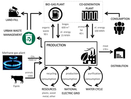
Figure 1.
Daily production for the case study of the meat industry in Italy.
The flows of animals and meat in the CLSC influence transportation and perishability costs, as well as charges of activities in logistic nodes. Consequently, the Net Present Value (NPV) of cash flows generated by all operations performed in the logistic chain could be evaluated, and quick reaction in real time without substantial time delay could be enabled if decisions and actions are possible because the data are available in real time as the events happen. The cost of flows between two nodes depends on their locations and the transportation mode used between them, as well as on the perishability characteristics of the meat in the chain. Important in this context are also the locations of the reverse logistics activities and disposal units.
An integrated meat supply chain includes the purchasing of animals and other raw materials, manufacturing with assembly, extracting, and distributing produced goods to other production units, or to the final clients—where consumption defines the activity levels—and finally to the reverse logistics activities (see Figure 1).
In a meat supply chain, critical variables under consideration for each operation are the activity level and timing, the inventory level, the perishability dynamics of meat, lead times, and other delays. The transformation of data of these physical indicators to the economic performances enables evaluation of control in a chain. The objective is to achieve the maximal net present value (NPV) of activities in the meat supply chain. By reducing the quantity of waste which goes into the environment, supply chains may also avoid costs of mitigating the pollution.
As written in [31], if managers of a supply chain do not have to bear them, market prices and the resulting NPV do not reflect these costs accurately. If the landfill is costly, it is reflected in the price vector c*, as will be explained later. Meat and other raw materials or components are delivered and stored in raw material warehouses at the production centers (slaughtering, processing, or repacking nodes). From there, they are transported in the required quantities to the next node of a graph representing the logistic system. There, the fresh meat and its components are transformed into semi-finished (prepared for packaging) goods, and so on. Here also the question is, how and when to include activities of the reverse logistics in a supply chain and how the increased percentage of recycling items in production affects the NPV of the total integrated chain. It is particularly difficult to evaluate NPV when lead times are varying simultaneously in the chain, and where the perishability dynamics are quite intensive and changing. The compact analyses in the frequency domain, in which lead-time perturbations may be studied analytically, make an evaluation of perishability and timing in NPV much easier [27,28]. The MRP approach gives us good theoretical and practical results. This approach can also be used for the extension of the analysis to distribution. In such cases, the transportation matrix is added in the system, when perishables would be in focus, especially to the reverse logistics part of a supply network further developed by [43]. Knowing better the data of parameters in the CLSC as presented in Figure 1, we can determine the values of decision variables and settings for improvements of NPV and related environmental criteria.
2.2. Monitoring and Control of the Perishability Dynamics in Meat Supply Chains—The Literature Review
Meat is one of the highly perishable cargos, which, unless adequately stored, processed, packaged, and transported, spoils quickly. Essential data which should be considered in the dataset are data on the quality of items in the flow of the supply chain and the value of things regarding their shelf-life [33]. The perishability dynamics of meat depends on various factors like pre-slaughter practices, age of the animal in the slaughtering process, handling during slaughtering, temperature controls during slaughtering, processing and distribution, preservation methods, packaging, and storage by consumer [25,44,45]. Different technical operations are involved in slaughtering actions following one after another in a supply chain of the meat industry. Inadequacy and therefore increased perishability at one stage results in a negative impact on the process and quality of items in the following stage [46]. The storage and transportation temperature, humidity and light, as well as the acidity of the meat and the structure of muscular tissue also affect the perishability dynamics [47] and therefore also cause the distribution of time to fall under the critical value of the shelf life. After a few hours of slaughtering, muscles become firm and rigid because of the stress during the slaughtering process. For controlling enzymatic, oxidative, and microbial spoilage, low-temperature storage and chemical techniques are the most common techniques in the industry today, but can often be perturbed so that the meat is exposed to the risk that it will not be bought. It is recommended to store the pieces of meat at lower than 4 °C immediately after slaughtering and during transport and storage, as it is critical for meat shelf life, appearance, and eating quality [48], and therefore this influences the final prices achieved on the market or costs of the reverse logistics. The characteristics of volatile compounds in meat in process differ so that each type of meat has its characteristic features, like odor and color, shelf-life, and the distribution of the time to the CRSL stipulated in the contract. Active packaging is one of the methods to extend the shelf-life of meat. Active materials absorb, for example, moisture and/or contain antimicrobial ingredients and antioxidants to improve the performance of meat. One of the most popular active packaging technologies is, for example, modified atmosphere packaging [49], which acts as a barrier against contaminants. Additionally, adding sensors to such a packaging system can also be considered so that we can detect earlier any event when perishability dynamics increase over expected limits. Namely, the sensors provide knowledge of freshness to alert increase of perishability dynamics in the packages of the fresh food or cold supply chain. This information requires our immediate action by changing temperature, humidity, or even to decide on a different final destination in time if we assume with a critical probability that the final customer will not buy the meat, which influences faster perishability dynamics. Such a combination is called “smart packaging”. The packaging system can detect, sense, and record any deterioration inside the meat package [50]. This way, we improve safety and quality. Namely, it enhances warning regarding deterioration processes during transportation, warehousing, and delivery to the final user [51,52]. Such control should be a part of the data-driven CPS of meat logistics.
2.3. Temperature and Humidity Measurement
The ATP Agreement [37] gives details on temperature measurements that need to be carried out, including the traceability of the measurements and also procedures for the thermal evaluation concerning prescribed insulation.
Perishables are not influenced only by temperature, but also by another crucial environmental parameter—humidity, and consequently, moisture [38]. Table 1 shows the optimal storage humidity for certain fruit and vegetables as presented in [53], and for meat by [46].

Table 1.
The optimal storage humidity and shelf life for certain fruit and vegetables compared to meat (not vacuum-packed).
Humidity can especially become an issue when vapor condenses during temperature shocks or uneven temperature/humidity distribution. Namely, a change in temperature by 1 °C can cause a relative humidity change, as high as 7 %, which could result in unwanted condensation for extended periods [54].
Therefore, if the humidity levels are close to condensing limits, it is important to note that temperature distribution inside the container alone can cause the condensation without being detected by the controlling thermometer. For this reason, proper and accurate humidity measurements are essential to implement. When taking into account the sharply defined natural threshold in humidity—the condensation—and the sensitivity mentioned above (up to 7%/°C), it is important to determine the target uncertainty of the measurements in order to be able to advise the optimal system control with respect to its cost and broad use. The characterization needs to be performed by precision state-of-the-art reference instruments, which are traceable to humidity measurement (physical) standards. This approach brings the need for implementation of a smart device that would measure and trace different environmental parameters.
Besides measuring, the device would also integrate geolocation with time-stamping and communication with the network cloud, as part of an Internet of Things (IoT). This integration would provide the base for real-time decision making and give ground for the recently introduced concept of ‘‘cold traceability’’ [42]. This concept helps to trace different groups of perishable goods like meat and other dairy products, which are transported under different cooling requirements.
The question arises, how can the cargo handling be improved to meet the final requirements? Additionally, what should be the conditions and restrictions of a dynamic system management be so that the final consumers will buy the food with a remaining shelf life (RSL) as long as stipulated in the contract? Are the static limitations of the perturbations at each moment as good as dynamic restrictions? To monitor the chain flows and to achieve the optimal control in the procedures of cooling and improvements, the skeleton of the model is built on the basis of input–output analysis in frequency domain, where timing is easier to manipulate and, in case of exceeding risk of improper delivery, the reverse logistics are included [43]. The results of cold chain management (CCM) are finally expressed and evaluated in the expected Net Present Value (NPV) of the final delivery to the buyer (with probability (1 − α) or to the local cogeneration plan (with probability α)). The impact of the risk of faster perishability and varying time delays is conveniently analyzed using NPV as the criterion function, derived from the annuity stream in the frequency domain. With the development of the IoT, the idea of moving activity cells with sensors has been presented in [33]. In this paper, the perishability dynamics of vegetables was assumed based on the variation of transportation lead time and other time delays at given changes in temperature. Currently, DHL is developing a technology for the next generation of cold chain visibility, forecasting near real-time visibility; full condition sensing, which monitors temperature and humidity, indicates shock and light; geo positioning; proof of delivery; and real-time alert notifications via SMS/e-mail [35]. These solutions would benefit from combining them with a decision support system, which would contribute to increasing the expected NPV (α) of activities in a supply chain. Besides, the measurements do not seem to consider all aspects of accurate humidity measurements. As described by [33] and written in [42], using smart devices that have multiple micro-sensors deployed in large quantities along the supply chains (including temperature and moisture detectors, as developed in our laboratory), we achieve a high capacity to trace and control perishable items in a variety of packages, pallets, parcels, or in bulk cargo in transport or storage.
In controlled environmental conditions, wireless sensors could measure physio-mechanical properties. Sensors have a long history, but having wireless sensors in cargo is relatively new. Regarding parcel boxes in Germany, where delivery points at home (domotics) also continue to multiply [35], logistics providers face new challenges. They need to find creative, cost-effective solutions that provide value for the end customer and operational efficiency for the logistics provider. Therefore, the IoT infrastructure for CPS as presented in [33] could create the “last mile” optimized collection from the mailboxes. Sensors placed inside the box detect whether it is empty and, if so, transmit a signal that is then processed in real time.
3. Modelling a Meat Supply Chain
3.1. Shelf Life (SL) of Meat and the Customer Remaining Shelf Life (CRSL)
Regarding perishable products, meat is among those with the shortest SL if the temperature is higher than 0. Therefore, production and logistics losses and waste should be considered carefully. In addition to regulations of fresh fruit and vegetables, meat has to be controlled [55], as given in EU Regulation 1169/2011. For the SL extension, there exist various packaging solutions, such as atmosphere and vacuum packaging [56]. In the meat supply chain, the quantity of waste is enormous, and therefore reverse logistics should also be organised like in Italy (see Figure 1). Freshness is strongly influenced by temperature and mode of aging (dependent on humidity). SL of the vacuum-packed beef at different temperatures is presented in Table 2.
Table 2.
Shelf life of the vacuum-packed (constant, optimal humidity) beef as a function of temperature.
Inadequate warehousing, transportation humidity, and temperature influence a costly reduction of the shelf life of meat cargo [57]. The results, as detected by the final customer, are the sensory characteristics of meat regarding odor, texture, and color. It can be measured by the sensory index (SI), which has its threshold at 1,8, but more precisely, the SL of meat depends on a number of microbes per gram of meat measured by colony-forming units per gram (cfu/g) of meat (Pseudomonas spp). [57] have determined the observed SL of meat as the time t when the Pseudomonas spp. reach 7,5 [log10cfu/g]. In many statistical observations, the Gompertz curve was used to describe the growth of microorganisms in meat, but unmodified exponential approximation or Weibull distribution is acceptable for our domain and the definition area. Therefore, we assume that the perishability in a node of a chain and between the nodes is described by:
- ∙ and
- ∙………
There are various reasons that meat in cold chains is exposed to the risk of reduced SL, such as pre-cooling of products, warehousing activities, and transhipments, waiting times during loading and unloading, and waiting in lines on the roads due to accidents or due to work on the road, or simply temperature abuses during transport. In many meat supply chains, only the environmental temperature at the truck level is monitored, from which it is not possible to draw reliable conclusions about the temperature inside the pallet or at the package level, because high variations could be detected inside a truck [58]. To obtain dispersed measurements inside the truck and their time series, an appropriate infrastructure for Big Data Analytics is needed. To determine the remaining SL and report the quality status at any moment in the chain, the graph of the chain should be known and the intensity of flows through the chain in any moment should be describable.
To estimate the present quality of meat and to be able to describe the future of perishability dynamics, a skeleton given by the MRP theory is suggested here. On this skeleton, the SL model is developed, which is based on the temperature and humidity monitoring devices. Organization of the meat supply chain from fields and stables to the final consumer depends on the number of animals in the source and the intensity of slaughtering in the slaughterhouse. In the case that a full truck can be loaded, the meat is transported from the slaughterhouse to the warehouse or distribution center directly (like in the numerical example). If the volume of the meat is less than a truck-full, the load of several suppliers should be first consolidated in a short time in depots and later transported to the warehouse or distribution center. A quality tracing in the food chain is possible, using wireless sensor networks, where sensors should be installed in slaughterhouses. A detector connected to the IoT is necessary, enabling temperature logs to calculate the RSL of the meat all along the supply chain. In case the remaining SL expected at the final user falls under the contracted level, the cargo should be redirected. Therefore, our aim was the development of a model for CPS of temperature-humidity-based quality control for meat that can be used for quality tracing along a meat supply chain and as a decision support tool to improve the NPV.
The remaining shelf life RSL(t) is the time from a certain moment t of measurement of the perishability level of meat and its environment (ambient conditions), until the final moment when the product is still acceptable for consumption by a customer. Because the perishability dynamics are a random variable, we can forecast the expected remaining shelf life—E(RSL(t + τ)). The sensors detect it, and CPS reports on it. Depending on the supply-chain ambient conditions, quality will decrease over time at varying rates, described here by perishability dynamics in the nodes . If the decay acceleration rate changes at the moment , we can write
where and is the index of a child node of the -th node on the route from time to . If the stipulated CRSL in the contract with the final customer is at a risk higher than the risk determined in advance (system’s risk aversion, SRA), the CPS could require a redirection of the flow from the chain to the nearest buyer for a lower price or to the reverse logistics sub-system, based on the known next admissible path on the MRP network.
3.2. Notation at Modification of the Extended MRP Theory and Required Data
We use the following notation for data, advised to be collected in the meat CLSC database, explained in the Table 3.
Table 3.
Notation and the required data.
3.3. The Skeleton Parallel to the Skeleton in the MRP Theory
There are four sub-systems and the processes are grouped into four sets of columns, representing production, distribution, consumption, and recycling respectively. The activity vectors are denoted: , concerning the respective processes of the sub-systems. Finally, denotes input requirements to the subsystem and outputs from sub-system k, k = 1, 2, 3, 4, so that a whole x may then be written as
Here, is the input matrix concerning the need of items required by sub-system k from running processes in sub-system l. Grey-colored elements of H in (2) would be zero matrices in a typical standard case. The net production is given by z, which is:
Table 4.
Net production sub-vectors (extension of [41]).
The quality of meat decreases in the supply chain with the perishability dynamics depending on temperature, humidity, and other environmental factors. The separation of good items from bad items is not possible during transportation, but only at the final delivery. CPS calculates the remaining shelf life only on the basis of the ambient parameters from a sensor attached to the pallets. Products have their shelf life from a farm to the end of usability, and a price of products p depends on the remaining shelf life (and is equal to c0 if RSL after the final delivery (CRLS) according to the stipulated contract).
3.4. The Economic Relationships of the Model
Items are assumed to have unit economic values which could be different in different nodes. If in the case that the cargo becomes suddenly highly exposed to risk of decay, and the smart devices recognize that the system could report to the nearest city which hosts the child node, and smart city can organize the transactions for such cargo locally at lower but acceptable prices or, in the worst case, the city can organize the disposal of rotten goods. Therefore, we shall write the unperturbed price vector c of items being a row vector:
determined at the standard shelf life of the items in the nodes , but in case of perturbations, the prices could be lower than or even negative if an immediate disposal is needed. Therefore, there exists a perturbed vector of lower or even negative prices (in case of landfill or in case of the waste incineration):
In the case of expecting a breach of contract when arriving to the final customer with a too high a probability when being on the arc , the rescheduling will be arranged. In this case, two events could happen: To sell the products on the local market of the node or to send it to the local cogeneration plant. Following the procedure of [30,31], we can write the NPV of a perturbed CSC at constant , where the basic generalized transportation input‒output matrix is given by (8). In this expression, we do not differentiate between the good and the bad cargo and keep them all on the vehicles from the stable to the final customer, following [30] and equation 14. Note that indexes belong to the reverse enumeration as in the papers of [27,28,29] and the recent paper of [59,60], where the cyclical processes repeat in constant time intervals before any perturbations, and are perturbed later, changing NPV:
In (6) and (7), and are the basic and the perturbed vectors of timing and density of activities as described in [30,31], and constant is the continuous interest rate. In our case, we model cyclical processes of logistics, repeating themselves in constant time intervals therefore, we must write in the frequency domain, the plan in the following way:
where is a vector of constant cargo sizes, for instance describing the total amounts to be delivered during one of the periods , j = 1, 2, …, n and where , j = 1, 2, …, m, are the points in time when the first of each respective cycle starts in node j when s = . If we have a single truck with the same load all the way and the unit of cargo is total cargo, the vector is and here means the standard notation for transposing the vector.
In the case of a supply chain as a chain through which the items make a certain path from a node to a node, the expression becomes much simpler, and we can write that the generalized matrix is:
Equation (10) will be shortly written as
In the case that CPS detect and calculate a high probability that CRSL will be too short, the redirection is ordered to a nearby location in the time distance τkf when being in the node k. Therefore, in case of perturbations only in perishability dynamics, the generalized matrix without perturbation in time delays changes to:
We shall write (12) shortly as:
and its perturbed case, when lead times are also perturbed, is therefore:
if it is redirected to the nearby consumption or disposal area.
In (6) and (7), the ordering and other setup + fixed production and distribution costs per unit of activity appear at each node, collected into the row vector of the setup costs
and column vectors of timing is:
where can be perturbed for and .
In the distribution part of a supply chain, it is often assumed that , but sometimes there could also be many sub-cycles of length T/m where m is number of deliveries in the next stage by smaller delivery vehicles that follow delivery with larger ones after the previous part of the route. To the NPV of repeated activities in (6) and (7), we have to also add transportation costs, as explained in the paper of [41], and further developed by [30,31] by including the transportation matrix. Congestion, which is increasing in national and international transportation networks, remains a serious problem, influencing matrix of time distances between nodes, and therefore influencing and the matrix of the perishability dynamics
The CPS control the perishability dynamic as a function of temperature and humidity at each nonempty arc , being exponentially distributed when the truck arrives in the arc , and learn the further development of perishability and calculate the probability that the cargo will arrive at the final destination with critical value of the remaining shelf life A or lower, where A is stipulated in the contract. To calculate it, we have to write the matrix of perishability dynamics. To clarify the case more explicitly, we shall assume the quantity on each arc needed for a unit of cargo in the next step with . In such a case, we can write the perishability dynamics as Time-spending distances give a better evaluation of transportation costs than the Euclidian or road distances, and can better measure the risk of events on the road when transport is slowed down or even stopped in a shorter time. The time-spending distance is included in the model. Between two fixed nodes of the graph, there is always a moving node which presents the movement of the truck. The moving node is equal to a child node if the perishability dynamics do not change. Between the location of the activity cell i and following activity cell j, transportation costs per item in transport could be determined by the product , where represents the transportation costs per unperishable item per time unit, which we collect into a transportation price matrix per unit of product transported so that the NPV of transportation costs between nodes on the transport route is equal to:
In (17), the row vector E is the vector of units (to summarize). are transportation costs from per item per time unit. If the source of items transported to j is only at one location, we have a simple case of a chain, (simple path in a directed graph) where and ,
3.5. Perturbations of the Chain on the Edges or in the Nodes of a Graph
In case of perturbations, the NPV is changed to:
where is the coefficient of increase of the transportation time on the arc ().
The matrix is a perturbed in timing with perturbations described shortly as
Let us now assume that when the cargo arrives somewhere on the arc () or in the node CPS calculate the CRSL and we realize that the perturbations in timing or in the perishability dynamics have been so high that the likelihood of the CRSLfalling under the critical value of the stipulated CRSL is higher than . We also assume that there is another customer in the node or very close to it who is willing to buy a product at a lower price . In this case, the transportation matrix is equal to
In case of such routing and in the case when the CPS detect a too high probability that the CRSL will fall under the contractually stipulated value, and therefore redirection in the node k is needed and possible, transportation costs are lower and the NPV of all such redirected transportation costs would be:
Here is the probability that in the node the cargo will be redirected to the near disposal area or final user, which is time units distance from node , and where the final income or disposal costs including the loss of final income would be . In such a meat logistic system, the total NPV is:
where the row vectors and have components from i=1 to k-1 equal to 0. Additionally, has the non-zero rows only from the row k+1 and further.
3.6. Net Present Value of the Repetitive Deliveries in a Supply Chain of Perishable Goods When the Critical Values of CRSL are Detected Earlier in the Chain
Let us now assume that the perishability dynamics on the chain with described in (10)–(13) and transportation costs matrix Π described in (15)–(17) with possible perturbations. In such a meat logistic system, the total NPV is given in (24). Like in (24), the row vectors and have components from i = 1 to k − 1 equal to 0. Additionally, has the non-zero rows only from the row k + 1 and further. CPS behave so that the NPV is maximum:
The CPS control the perishability dynamic as a function of temperature and humidity at each nonempty arc , being often exponentially or Weibull distributed when the truck arrives in the arc , and learn the further development of perishability and calculate the probability that the cargo will arrive to the final destination with a critical value of the remaining shelf life A or lower, where A is stipulated in the contract. To calculate it, we have to write the matrix of perishability dynamics. To clarify the case more explicitly, we shall assume the quantity on each arc needed for a unit of cargo in the next step with . In such a case we can write:
As given in [18,19], about 20% of meat is wasted according to an estimate made by the United Nations. As explained in [18], every kilogram of meat needs up to 130 times more water than a kilogram of potatoes and up to nine times more CO2 is produced. Therefore, the reduction of meat waste suggested by this procedure is evident. Reducing the mileage of trucks transporting this meat when food is no longer usable at the destination, additionally contributes to environmental health (reduces pollution) and ecosystem vitality, all of which contribute to raising the Environmental Performance Index (EIP). Taking into account Formulas (19)–(23), by substituting the coefficient b for the pollution indicator, we can also see how this innovation contributes to raising the environmental performance index.
4. The Example, Where the Only Path on the Graph is a Chain
We shall consider the published case of [44]. They developed a quality tracing procedure for vacuum-packed lamb. They calculated relevant sensory parameters, and the results have been used in the predictive model. Over the long term, their procedure was able to support the reduction of food waste and improve the resources efficiency of food production.
The authors analyze a cold chain of Irish lamb products including cross-docking facilities (depot and warehouse) with nodes and transportation roads as given in Table 5 (see the details in [44], Table 2). In their case study, the delivery of lamb products from the producer in Ireland to the customer in Germany could take even only 90 h, but may vary on the timing (in the presented case study the transportation and other logistics are 168 h long), and also the temperature of cargo can rise above . Suppose that the cargo is collected at the port of departure, as a node 4 so that the initial RSL is only 406 h. A visual respresentation of the dependence of shelf life on temperature is given in Figure 2 and a cold chain path is presented in Figure 3.
Table 5.
Deterioration of the lamb cold chain on the transport route from Dublin to Bremen. The contract stipulated CRSL = 240 h, and CRSL in the initial node is equal to 406 h.
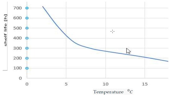
Figure 2.
Shelf life (SL) of vacuum-packed lamb in dependence of cargo temperature.
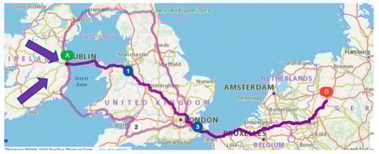
Figure 3.
An example of transportation of the lamb cold chain on the route from Dublin to Bremen, just to node 2.
Let us consider how this procedure could be controlled using our method, if the initial RSL was 406 h and the price in the contract was 150,000 Eur per unit (one truck) in case of contractually stipulated CRSL 230 h or more, and the cargo is refused in case of lower CRSL. However, in case of the probability of a lower CRSL at the final node, there is a possibility only at the wholesaler (node 2) that the cargo is redirected to an another customer, who is willing to buy the products for 50,000 Eur per unit in the case that it is not completely rotten. Let us consider what would be the decisions of our managers, based on our proposed procedure.
In case of the optimal temperature of cargo from the origin of this transport road in Ireland to the destination in Germany, the average perishability dynamics were assumed to be equal to:
While regarding the requirements stipulated in the contract (CRSL ≥ 230 h), the maximum of allowed is max 0.003383, there is a high probability that even in the case of optimal maintenance of the temperature in the cargo and in the case when the time of transport and other logistics do not increase, as in the case of perturbations in Table 5, there is a high probability that CRSL falls below the contract value, therefore the managers will consider to redirect the cargo in the node 2. The CPS controls the perishability dynamic in transportation and in nodes as a function of temperature and humidity at each non-empty arc , being exponentially distributed when the truck arrives in the arc , learns the further development of perishability, and calculates the probability that the cargo will arrive at the final destination with a critical value of the customer’s remaining shelf life CRSL = 240 h as stipulated in the contract. To calculate it, we have to write the matrix of perishability dynamics.
To clarify the case more explicitly, we shall assume the quantity on each arc needed for a unit of cargo in the next step with (means, for example, one S.KO COOL box body semi-trailer with 30,000 kg of cargo). In such a case, we can write:
Regarding the case in Table 5, the values ) and are given in the column VI, the values of are written in column VII for unperturbed transportation and other logistics, and in column X in the perturbed case.
There exists a particular critical value at which the cargo will be rejected by the final costumer with probability depending on the distribution of RSL (t +. In the case that CPS recognise (in the arc or in the node that the probability that the value of CRSL is lower than agreed in the contract and is higher than α, redirection is required to the nearest landfill, waste incinerator, or—if good enough—to the nearest market.
Let us assume that in the case reported in Table 5 there is possible cargo diversion only in node 2, where it is sold for a half price with probability or disposed of in a waste incinerator with probability for which it is necessary to pay 1000 € per unit of cargo. The probability of continuing to the final destination (to the node 1) is therefore 1 − calculated from the history of these activities, knowing perishability dynamics in the case of optimal and perturbed temperature control like in Table 5, as well as probabilities of perturbations caused by timing, which can often be reported also by some apps and linked with our CPS. At the end customer, the cargo may again be acceptable with an probability, or it may again need to be taken to incineration with probability . We may write for this particular case that = = 1.
If CPS follow this policy, then the whole NPV () in this case would be as given in (24). Let us suppose the following values of parameters:
- ⚬
- Price vectors are: ]; ];
- ⚬
- the price of waste incineration in node 1 is equal to the price in the node 2:
- ⚬
- the formulation of logistic dynamics in cold chains is expressed much more simple than a general production MRP formulation, since ;
- ⚬
- ;
- ⚬
- at a given continuous interest rate and the time to disposal or earlier delivery at node 2 is 1 h from the warehouse (=1), the matrices H are:
- ⚬
- the transportation costs matrices are:
After calculating maximum likelihood (MLE) values of on the bases of their own historical data, description of the current load condition, and on the reports on the environmental conditions on the roads, expected can alsobe calculated.
T = 1 week = 168 h and the values of α are the following:
With the chosen perishability dynamics, as given in the column VII of Table 5, and with timing, presented in column III of the same table, we have got:
Here we calculate:
Time unit in our case is 1 h and we suppose the continuous daily interest rate .
CPS can adapt to new parameters whenever the changes are detected. We compare this value with the expected value to sell the cargo at the local market or to dispose of it and decide on rescheduling, calculating NPV on the submatrices from 1 to n−1. If the rescheduled case gives a higher expected value, a redirection is made. The CPS also automatically sends the note to the stakeholders.
The countries through which this supply chain runs have the environmental performance index higher than 70, some even higher than 80. Taking into account Formulas (19)–(23), by substituting the coefficient b for the value of the pollution indicator, we can also see how this innovation contributes to raising the environmental performance index.
5. Conclusions and Directions to Further Research
Supply chain management of repeated shipments of perishable food requires a more intelligent technology to improve post-harvest loss prevention, to reduce lead times, and control perishability dynamics or at least reduce the transportation costs in case perishability dynamics become exposed to the high risk of achieving Customer Remaining Shelf Life at the final destination. We have seen that a higher income of total supply chain alliance of managers (as suggested by WEF in Davos in 2013) can be achieved by developing broader and more accurate planning and control of perishability together from stable to fork, providing/offering possibilities to redirect the shipments in case of increasing perishability dynamics or inordinately high time delays on the roads. In the meat supply chain, substantial losses may occur throughout the whole route. We presented how a substantial value may be added to the NPV as the criterion function by possibilities of rescheduling the remaining route in case of immediate, real-time detection of changes in (a) time delays in the system, (b) perishability dynamics, or (c) both at the same time. The procedures suggested here include a real-time calculation and communication of the remaining shelf life during transportation and other logistic manipulations from one chain node to another, all to the final user if the time to exceed the contractually stipulated Customer Remaining Shelf Life is distributed by known distribution. The changes in the estimated RSL should, therefore, be detected immediately, and the remaining route rescheduled if necessary.
Planning and control of meat shipment on the skeleton of the extended MRP model are advised, and the role of the collaborative cities in the network of final users is presented. In the model, we show how improvements can be achieved by the dynamic rerouting in real-time, based on the risk valuation. The changes in NPV at contractually stipulated Customer Remaining Shelf Life are calculated dynamically in real-time. We have explained how the Internet of Things (IoT) enables such real-time reports. Smart devices, tracking temperature, humidity, and gas concentration, allow such reports immediately after the detection of changes influencing the parameters of the Weibull distribution of shelf life on each directed edge or in a node of the graph can be forecasted. The model includes the assumption of possibilities to deliver the meat to the local market or even to the reverse logistics plants in the nodes of the remaining route if the expected contractually stipulated Customer Remaining Shelf Life becomes too high. In the numerical examples, a case is given on how much such a cyber-physical system improves NPV of the meat supply chain by this decision support model. We are also answer the question of how the results are improved with direct delivery in the smart refrigerator, which is especially convenient for older customers supplied by such meat supply chain.
In the presented model, we focused mainly on the issue of economic sustainability of meat supply through the evaluation of NPV of this supply in case of exposure to the risk of spoilage of meat during a long-distance transport, but in our formulas, there are also indicators which contribute to the environmental sustainability. Reducing food losses due to spoilage processes, as well as reducing the length of unnecessary transportation routes for meat trucks, improve the objectives of the environmental performance index. Thus, in further studies, it is possible to move from a single-criteria function that supports decisions regarding economic criteria, to a bi-objective function, when we add to the current formula the environmental health and ecosystem vitality measures and goals that contribute to raising EPI as another optimization objective. Taking into account Formulas (19)–(23), by substituting the coefficient b for the pollution indicator, we can also observe in parallel how this innovation contributes to raising the environmental performance index. This direction will be the subject of our further research.
Organizing smaller groups of customers on the transport route from the source of the meat to the intended end-user would be a good solution to reduce the risk of spoilage of the meat on the transport route when the meat is still of good quality on the part of the route, but is less likely to reach contractually agreed CRSL at the end of this road. For such cases, we studied that the organization of retirement communities and schools along the way to buy this meat at significantly reduced prices, but still of high quality, would be a favorable solution for the care systems of the elderly, which additionally contribute to the social sustainability of eldercare.
The automatic redirection of meat and meat products in the cargo is based on the assumption that the exponential or Weibull Reliability Function can be used when modelling reliability and risk of proper delivery according to the stipulated contract. It is assumed that the Big Data are created through automatic identification sensors of humidity and temperature, from where the parameters of reliability functions are determined, and exposure to risk is evaluated. Such procedures can be developed now when the Internet of Things applications are growing very fast in industrial engineering.
In this paper, we assumed that repeated flows appear on the infinite horizon, which is not often the case. Additionally, when developing the network of customers in the settlements on the road, the costs of developing such a network should be compared with the expected increase in NPV for the case of established collaborative networks. If the activity of a supply chain appears on a reasonably short time horizon, the correction which is the result of the final length of the tasks on the horizon should be evaluated. Therefore, we must find the correction factor which could be calculated using some Network Simulation Model [61,62,63], which has already been applied successfully in several fields of engineering, such as electrochemical reactions, heat transfer, and many others. These improvements will be the subject of our further research in cooperation with the Universidad Politécnica de Cartagena, where the simulation lab is available.
Author Contributions
D.B. and M.B. conceptualized the methodology; D.B. developed software, lead the research; D.H. developed measurement tools and wrote the draft of Section 2.1 and Section 2.3, S.C. wrote the final text of this article, and prepared presentation; M.B. also edited the paper including validation of the model. The research was running under the guidance of V.D. All authors have read and agreed to the published version of the manuscript.
Funding
This research has received funding from the European Union’s Horizon 2020 research and innovation program under the Marie Sklodowska-Curie grant agreement No 873077 (MAIA-H2020-MSCA-RISE 2019).
Conflicts of Interest
The authors declare no conflict of interest.
References
- Lambert, D.M.; Enz, M.G. Issues in Supply Chain Management: Progress and potential. Ind. Mark. Manag. 2017, 62, 1–16. [Google Scholar] [CrossRef]
- Hartmann, J.; Moeller, S. Chain liability in multitier supply chains? Responsibility attributions for unsustainable supplier behavior. J. Oper. Manag. 2014, 32, 281–294. [Google Scholar] [CrossRef]
- Panigrahi, S.S.; Bahinipati, B.; Jain, V. Sustainable supply chain management. Manag. Environ. Qual. 2019, 30, 1001–1049. [Google Scholar] [CrossRef]
- Gold, S.; Seuring, S.; Beske, P. The constructs of sustainable supply chain management—A content analysis based on published case studies. Prog. Ind. Ecol. Int. J. 2010, 7, 114. [Google Scholar] [CrossRef]
- Seuring, S.; Sarkis, J.; Müller, M.; Rao, P. Sustainability and supply chain management—An introduction to the special issue. J. Clean. Prod. 2008, 16, 1545–1551. [Google Scholar] [CrossRef]
- Grimm, J.H.; Hofstetter, J.S.; Sarkis, J. Exploring sub-suppliers’ compliance with corporate sustainability standards. J. Clean. Prod. 2016, 112, 1971–1984. [Google Scholar] [CrossRef]
- Venkatesh, V.; Kang, K.; Wang, B.; Zhong, R.Y.; Zhang, A. System architecture for blockchain based transparency of supply chain social sustainability. Robot. Comput. Manuf. 2020, 63, 101896. [Google Scholar] [CrossRef]
- Bansal, P. Evolving sustainably: A longitudinal study of corporate sustainable development. Strat. Manag. J. 2005, 26, 197–218. [Google Scholar] [CrossRef]
- Zhu, Q.; Sarkis, J.; Lai, K.-H. Confirmation of a measurement model for green supply chain management practices implementation. Int. J. Prod. Econ. 2008, 111, 261–273. [Google Scholar] [CrossRef]
- Green, K.W.; Zelbst, P.J.; Meacham, J.; Bhadauria, V.S. Green supply chain management practices: Impact on performance. Supply Chain Manag. Int. J. 2012, 17, 290–305. [Google Scholar] [CrossRef]
- Green, K.W.; Inman, R.A.; Sower, V.E.; Zelbst, P.J. Impact of JIT, TQM and green supply chain practices on environmental sustainability. J. Manuf. Technol. Manag. 2019, 30, 26–47. [Google Scholar] [CrossRef]
- Florida, R.; Davison, D. Gaining from Green Management: Environmental Management Systems inside and outside the Factory. Calif. Manag. Rev. 2001, 43, 64–84. [Google Scholar] [CrossRef]
- Vachon, S.; Mao, Z. Linking supply chain strength to sustainable development: A country-level analysis. J. Clean. Prod. 2008, 16, 1552–1560. [Google Scholar] [CrossRef]
- Deng, X.; Yang, X.; Zhang, Y.; Li, Y.; Lu, Z. Risk propagation mechanisms and risk management strategies for a sustainable perishable products supply chain. Comput. Ind. Eng. 2019, 135, 1175–1187. [Google Scholar] [CrossRef]
- Diop, N.; Jaffee, S.M. Fruits and vegetables: Global trade and competition in fresh and processed product markets. In Global Agricultural Trade & Developing Countries; Aksoy, M., Ed.; World Bank: Washingtion, DC, USA, 2005; pp. 237–257. [Google Scholar]
- Noya, I.; Aldea, X.; Gasol, C.M.; González-García, S.; Amores, M.J.; Colón, J.; Ponsá, S.; Roman, I.; Rubio, M.A.; Casas, E.; et al. Carbon and water footprint of pork supply chain in Catalonia: From feed to final products. J. Environ. Manag. 2016, 171, 133–143. [Google Scholar] [CrossRef] [PubMed]
- Wang, J.; Liu, S.; Su, J. Identifying vulnerable nodes in supply chain based on the risk transmission model. In Proceedings of the 6th International Conference on Industrial Technology and Management, Cambridge, UK, 7–10 March 2017. [Google Scholar]
- Sprong, J.; Lin, X.; Maestre, J.; Negenborn, R. Quality-Aware Control for Optimizing Meat Supply Chains. In Proceedings of the 18th European Control Conference, Naples, Italy, 25–28 June 2019. [Google Scholar]
- Food and Agriculture Organization (FAO). Per Capita Egg Consumption. 2017. Available online: https://ourworldindata.org/meat-production#per-capita-egg-consumption (accessed on 3 April 2020).
- Raab, V.; Petersen, B.; Kreyenschmidt, J. Temperature monitoring in meat supply chains. Br. Food J. 2011, 113, 1267–1289. [Google Scholar] [CrossRef]
- Arason, S.; Asgeirsson, E.I.; Margeirsson, B.; Margeirsson, I.; Olsen, P.; Stefansson, H. Decision support systems for the food industry. In Handbook of Decision Making; Jain, L.C., Lim, C.P., Eds.; Springer: Berlin, Heidelberg, 2010; pp. 295–315. [Google Scholar] [CrossRef]
- Andriolo, A.; Battini, D.; Calzavara, M.; Gamberi, M.; Peretti, U.; Persona, A.; Pilati, F.; Sgarbossa, F. New RFID pick-to-light system: Operating characteristics and future potential. Int. J. RF Technol. Res. Appl. 2016, 7, 43–63. [Google Scholar] [CrossRef]
- Azzi, A.; Battini, D.; Persona, A.; Sgarbossa, F. Packaging Design: General Framework and Research Agenda. Packag. Technol. Sci. 2012, 25, 435–456. [Google Scholar] [CrossRef]
- Battini, D.; Bortolini, M.; Faccio, M.; Regattieri, A. Energy and cost optimization in multi-modal fresh food distribution network. In Proceedings of the 22nd International Conference on Production Research, Parana, Brazil, 28 June–1 August 2013. [Google Scholar]
- Battini, D.; Calzavara, M.; Persona, A.; Sgarbossa, F. Sustainable Packaging Development for Fresh Food Supply Chains. Packag. Technol. Sci. 2015, 29, 25–43. [Google Scholar] [CrossRef]
- Yang, S.; Xiao, Y.; Kuo, Y.-H. The Supply Chain Design for Perishable Food with Stochastic Demand. Sustainability 2017, 9, 1995. [Google Scholar] [CrossRef]
- Grubbström, R.W.; Tang, O. An Overview of Input-Output Analysis Applied to Production-Inventory Systems. Econ. Syst. Res. 2000, 12, 3–25. [Google Scholar] [CrossRef]
- Grubbström, R.W. Transform methodology applied to some inventory problems. J. Bus. Econ. 2007, 12, 3–25. [Google Scholar] [CrossRef]
- Grubbström, R.W.; Bogataj, L.; Bogataj, M. A Compact Representation and Optimisation of Distribution and Reverse Logistics in the Value Chain. In Mathematical Economics, Operational Research and Logistics; Bogataj, L., Ros Mcdonell, L., Eds.; Faculty of Economics: Ljubljana, Slovenia, 2007. [Google Scholar]
- Bogataj, M.; Grubbström, R.W. On the representation of timing for different structures within MRP theory. Int. J. Prod. Econ. 2012, 140, 749–755. [Google Scholar] [CrossRef][Green Version]
- Bogataj, M.; Grubbström, R.W. Transportation delays in reverse logistics. Int. J. Prod. Econ. 2013, 143, 395–402. [Google Scholar] [CrossRef]
- Lee, J.; Bagheri, B.; Kao, H.-A. A Cyber-Physical Systems architecture for Industry 4.0-based manufacturing systems. Manuf. Lett. 2015, 3, 18–23. [Google Scholar] [CrossRef]
- Bogataj, D.; Bogataj, M.; Hudoklin, D. Mitigating risks of perishable products in the cyber-physical systems based on the extended MRP model. Int. J. Prod. Econ. 2017, 193, 51–62. [Google Scholar] [CrossRef]
- Mexis, S.F.; Kontominas, M.G. PACKAGING: Active Food Packaging. Encyclopedia of Food Microbiology, 2nd ed.; University of Ioannina: Ioannina, Greece, 2014; pp. 999–1005. [Google Scholar]
- DHL Parcel Delivery Boxes Now in Apartment Buildings. Available online: https://www.dhl.com/en/press/releases/releases_2015/group/dhl_parcel_delivery_boxes_now_in_apartment_buildings.html (accessed on 10 September 2020).
- Commission Directive 92/2/EEC. Available online: https://eur-lex.europa.eu/legal-content/EN/TXT/?uri=celex:31992L0002 (accessed on 2 September 2020).
- Agreement on the International Carriage of Perishable Foodstuffs and Special Equipment to be Used for such Carriage. Available online: https://www.unece.org/fileadmin/DAM/trans/main/wp11/ATP_publication/ATP-2016e_-def-web.pdf (accessed on 5 September 2020).
- Hudoklin, D.; Bojkovski, J.; Nielsen, J.; Drnovsek, J. Design and validation of a new primary standard for calibration of the top-end humidity sensors. Measurement 2008, 41, 950–959. [Google Scholar] [CrossRef]
- Beges, G.; Rudman, M.; Drnovsek, J. Evaluation of Flat Surface Temperature Probes. Int. J. Thermophys. 2010, 32, 396–406. [Google Scholar] [CrossRef]
- Pušnik, I.; Drnovšek, J. Infrared ear thermometers—Parameters influencing their reading and accuracy. Physiol. Meas. 2005, 26, 1075–1084. [Google Scholar] [CrossRef]
- Bogataj, D.; Bogataj, M. The role of free economic zones in global supply chains—A case of reverselogistics. Int. J. Prod. Econ. 2011, 131, 365–371. [Google Scholar] [CrossRef]
- Internet of Things in Logistics. DHL Trend Research. Available online: http://www.dhl.com/en/about_us/logistics_insights/dhl_trend_research.html (accessed on 6 September 2020).
- Net present value evaluation of energy production and consumption in repeated reverse logistics. Technol. Econ. Dev. Econ. 2015, 23, 877–894. [CrossRef]
- Mack, M.; Dittmer, P.; Veigt, M.; Kus, M.; Nehmiz, U.; Kreyenschmidt, J. Quality tracing in meat supply chains. Philos. Trans. R. Soc. 2014, 372, 999–1005. [Google Scholar] [CrossRef] [PubMed][Green Version]
- Sgarbossa, F.; Russo, I. A proactive model in sustainable food supply chain: Insight from a case study. Int. J. Prod. Econ. 2017, 183, 596–606. [Google Scholar] [CrossRef]
- Animal Production and Health. Good Practices for the Meat Industry. Available online: http://www.fao.org/docrep/004/t0279e/T0279E00.htm#TOC (accessed on 5 September 2020).
- Berkel, B.M.; Boogard, B.V.; Heijnen, C. Preservation of fish and meat. Agromisa Found. 2004, 8, 78–80. [Google Scholar]
- Mutwakil; Dave, D.; Ghaly, A.E. Meat Spoilage Mechanisms and Preservation Techniques: A Critical Review. Am. J. Agric. Biol. Sci. 2011, 6, 486–510. [Google Scholar] [CrossRef]
- Smiddy, M.; Papkovsky, D.; Kerry, J. Evaluation of oxygen content in commercial modified atmosphere packs (MAP) of processed cooked meats. Food Res. Int. 2002, 35, 571–575. [Google Scholar] [CrossRef]
- Kuswandi, B.; Jayus; Oktaviana, R.; Abdullah, A.; Heng, L.Y. A Novel On-Package Sticker Sensor Based on Methyl Red for Real-Time Monitoring of Broiler Chicken Cut Freshness. Packag. Technol. Sci. 2014, 27, 69–81. [Google Scholar] [CrossRef]
- Salinas, Y.; Ros-Lis, J.V.; Vivancos, J.-L.; Martínez-Máñez, R.; Marcos, M.D.; Aucejo, S.; Herranz, N.; Lorente, I. Monitoring of chicken meat freshness by means of a colorimetric sensor array. Analyst 2012, 137, 3635–3643. [Google Scholar] [CrossRef]
- Salinas, Y.; Ros-Lis, J.V.; Vivancos, J.-L.; Martínez-Máñez, R.; Marcos, M.D.; Aucejo, S.; Herranz, N.; Lorente, I.; Garcia, E. A novel colorimetric sensor array for monitoring fresh pork sausages spoilage. Food Control. 2014, 35, 166–176. [Google Scholar] [CrossRef]
- Paull, R. Effect of temperature and relative humidity on fresh commodity quality. Postharvest Biol. Technol. 1999, 15, 263–277. [Google Scholar] [CrossRef]
- Kentved, A.B.; Heinonen, M.; Hudoklin, D. Practical Study of Psychrometer Calibrations. Int. J. Thermophys. 2012, 33, 1408–1421. [Google Scholar] [CrossRef]
- Regulation (EU) No 1169/2011. Available online: https://eur-lex.europa.eu/legal-content/EN/ALL/?uri=CELEX%3A32011R1169 (accessed on 3 September 2020).
- Kiermeier, A.; Tamplin, M.; May, D.; Holds, G.; Williams, M.; Dann, A. Microbial growth, communities and sensory characteristics of vacuum and modified atmosphere packaged lamb shoulders. Food Microbiol. 2013, 36, 305–315. [Google Scholar] [CrossRef] [PubMed]
- Bruckner, S.; Albrecht, A.; Petersen, B.; Kreyenschmidt, J. Influence of cold chain interruptions on the shelf life of fresh pork and poultry. Int. J. Food Sci. Technol. 2012, 47, 1639–1646. [Google Scholar] [CrossRef]
- Raab, V.; Bruckner, S.; Beierle, E.; Kampmann, Y.; Petersen, B.; Kreyenschmidt, J. Generic model for the prediction of remaining shelf life in support of cold chain management in pork and poultry supply chains. J. Chain Netw. Sci. 2008, 8, 59–73. [Google Scholar] [CrossRef]
- Bogataj, L. Preface. In Input-Output Analysis and Laplace Transforms in Material Requirements Planning; Bogataj, L., Grubbström, R.W., Eds.; FPP: Portorož, Slovenia, 1998. [Google Scholar]
- Bogataj, D.; Battini, D.; Calzavara, M.; Persona, A. The Response Latency in Global Production and Logistics: A Trade-off Between Robotization and Globalization of a Chain. Procedia Manuf. 2019, 39, 1428–1437. [Google Scholar] [CrossRef]
- Marín, F.; Alhama, F.; Moreno, J. Modelling of stick-slip behaviour with different hypotheses on friction forces. Int. J. Eng. Sci. 2012, 60, 13–24. [Google Scholar] [CrossRef]
- Marín, F.; Alhama, F.; Meroño, P.A.; Moreno, J.A. Modelling of stick–slip behaviour in a Girling brake using network simulation method. Nonlinear Dyn. 2016, 84, 153–162. [Google Scholar] [CrossRef]
- Alhama, F.; Marín, F.; Moreno, J. An efficient and reliable model to simulate microscopic mechanical friction in the Frenkel–Kontorova–Tomlinson model. Comput. Phys. Commun. 2011, 182, 2314–2325. [Google Scholar] [CrossRef]


Publisher’s Note: MDPI stays neutral with regard to jurisdictional claims in published maps and institutional affiliations. |
© 2020 by the authors. Licensee MDPI, Basel, Switzerland. This article is an open access article distributed under the terms and conditions of the Creative Commons Attribution (CC BY) license (http://creativecommons.org/licenses/by/4.0/).