Injection Mold Production Sustainable Scheduling Using Deep Reinforcement Learning

Abstract

In the injection mold industry, it is important for manufacturers to satisfy the delivery date for the products that customers order. The mold products are diverse, and each product has a different manufacturing process. Owing to the nature of mold, mold manufacturing is a complex and dynamic environment. To meet the delivery date of the customers, the scheduling of mold production is important and is required to be sustainable and intelligent even in the complicated system and dynamic situation. To address this, in this paper, deep reinforcement learning (RL) is proposed for injection mold production scheduling. Before presenting the RL algorithm, a mathematical model for the mold scheduling problem is presented, and a Markov decision process framework is proposed for RL. The deep $Q$-network, which is an algorithm for RL, is employed to find the scheduling policy to minimize the total weighted tardiness. The results of experiments demonstrate that the proposed deep RL method outperforms the dispatching rules that are presented for minimizing the total weighted tardiness.

1. Introduction

In Industry 4.0, manufacturing companies consider technical issues [1] in addition to economic, environmental, and social issues [2] for sustainability. By considering the technical impacts on manufacturing, the manufacturers try to satisfy customer demand and to improve the production efficiency for enhancing sustainability. Among the diverse factors for achieving their endeavor, the agility or the flexibility of manufacturing plays an important role. If the manufacturers do not cope with a dynamic manufacturing environment with agility, it may lead to customers’ dissatisfaction and a decrease in the competitiveness of the manufacturers in the market. In Industry 4.0, the core of decision-making in manufacturing operations is based on information accessibility at the right time, which assists and enables the maintenance of manufacturing agility. With an increased utilization of the information, gathering and inferring industrial data, evolved intelligent production planning, scheduling, and control systems are required. Combining new technologies in Industry 4.0 with manufacturing processes, the performance of the systems is enhanced through real-time, data-driven, and continuous learning from a more varied range of data sources [3].

Among them, scheduling is a core process for manufacturing companies to maximize profits and to reduce costs at the same time. In particular, in a complex system and a dynamic manufacturing environment, more sustainable and intelligent scheduling that can respond to them is needed because poor scheduling has higher costs, a longer production time, and higher tardiness. Thus, to deal with a manufacturing site’s complexity and to improve its effectiveness, scheduling needs to be evolved and improved for sustainability and intelligence.

Injection mold (hereafter mold) manufacturing is a complex production system. Molds are used as the semifinal or final parts that can produce products for most firms. This is a special case where producing products are used in manufacturing processes for other industries such as automobiles, shoes, and electronics. As mold manufacturing plays an important role in the industry, mold manufacturing has been the focus of many studies in terms of the design process, manufacturing, testing the molds, and tuning the parameters of the molding machines [4]. These studies have focused on manufacturing to improve the quality of the manufacturing molds. Although it is important to look after the quality of the products for customer satisfaction, delivering the products on time is a matter of satisfaction for the customers as well.

The complexity of the mold manufacturing production system comes from a multi-product production system that is based on the customers. The products can be of many different types, and their processes vary from product to product. In addition, the processing time is dependent on the manufacturing line and generally ranges from a minute to hours. Therefore, scheduling to determine the allocation of jobs for machines is crucial. The demand and type of products are dependent on the customers, and satisfying the due date plays an important role in determining competitiveness in the mold industry. The mold industry is a typical multi-time, small-sized production. Some of the typical issues include frequent setup time occurrences, complicated processes, and planning for delays due to an urgent order and a dynamic environment. Therefore, developing effective and intelligent scheduling that can counteract flexibly while considering the products’ due date and the diverse product types in a dynamic environment is necessary for the mold industry.

In this study, to address the complexity and dynamic environment of mold manufacturing, deep reinforcement learning (RL) is employed for the mold scheduling problem. This study developed a scheduling method that uses the deep $Q$-network (DQN) as the algorithm for deep RL, which is applied to the scheduling for mold manufacturing systems. The state, action, and reward are defined properly for the mold scheduling problem. In the training section, the DQN is learned during the episodes, which are iterations for the mold scheduling problem. Once the training is finished, the performance of the proposed algorithm is evaluated by using dispatching rules for minimizing the total weighted tardiness.

The remaining sections of this study are as follows. Section 2 is the literature review of the mold manufacturing industry and deep RL. In Section 3, the mathematical model is presented to explain the mold scheduling problem, the Markov decision process (MDP) framework is proposed for RL, and the algorithm of deep RL is described. Section 4 presents the result of experiments, which are implemented through a case study. The discussion and conclusion are presented in Section 5 and Section 6, respectively.

2. Literature Review

2.1. Mold Manufacturing

As the mold is a core part of the diverse manufacturing industry, numerous studies have been conducted to improve production efficiency and enhance sustainability in the market. Low and Lee [5] focused on the cavity layout design system for the injection mold. The cavity is the main one among diverse parts that constitute the mold. As time-to-market for plastic products is getting shorter, the available time for mold manufacturing is decreasing. By making a template for designing the cavity layout, miscommunication was avoided between product and mold designers, and time was saved. Hu and Masood [6] exploited the intelligent cavity layout design system to assist mold designers in the cavity design step. Fu et al. [7] dealt with the parting surface, core, and cavity blocks in the computer-aided mold design system, which is the bottleneck. The architecture of the mold design system and the methodology to generate them were proposed.

Other studies addressed the layout design of the cooling system for the mold as the cooling step takes a large portion of the mold manufacturing process. The cooling system is important for the productivity of the process and the quality of the mold. Li et al. [8] developed a graph traversal algorithm to make cooling circuits from the graph structure that was devised to capture a given initial design. The heuristic search and fuzzy framework were used for developing the cooling circuits into the layout designs and evaluating the designs. Liang [9] derived the optimization model to achieve the highest transfer efficiency of the cooling system. Li et al. [10] used a topology optimization to design the conformal cooling system for the mold and simplified the analysis of the cooling process by the cycle averaged approach. The boundary element method was employed to find solutions and to calculate the sensitives.

Some authors have addressed the perspective of energy saving, as energy consumption is related to the company’s cost as well as environmental impacts. Li et al. [11] figured out the relationship between energy consumption and process parameters on mold machine tools via experimental observations in the research. With the observations, the throughput rate was found to be a critical factor for the energy and eco-efficiency of mold processes. Another study discussed the guideline to characterize the energy consumption of the mold process [12]. Five steps were presented for the guideline to calculate the estimated energy consumption. With the guideline, it could estimate and benchmark a variety of manufacturing processes and products using mold process by considering theoretical minimum energy that was computed with part design, material, and process planning, the estimation of energy consumption that was calculated with manufacturing resource information. Thus, many studies have been conducted from a variety of perspectives to improve the efficiency and sustainability of the company. However, as mentioned, as the mold products are used in other manufacturing as parts, the customer-oriented operational view of studies needs to be discussed. Based on the customer-oriented operation, the scheduling is a core process as it decides the number and the type of the product to manufacture, which leads to the demand of the customers.

In the literature, a few studies have approached mold scheduling with a variety of objectives. The mold scheduling problem has been formulated diversely, such as parallel machine scheduling, flexible job shop scheduling, and resource-constraint project scheduling problems.

Past studies [13,14] have addressed scheduling injection molding with production planning. The production plan was used as the input for the scheduling, and the heuristic method was developed for a scheduling problem by minimizing the makespan. Some authors have employed a meta-heuristic algorithm for mold scheduling. Oztemel et al. [15] developed a bee algorithm for multi-mode resource-constrained project scheduling in the mold industry to minimize the mold project duration. Wang et al. [16] used an ant colony optimization algorithm for the selection of machines that are needed in each working procedure, and the job sequence was determined by the heuristic algorithm. Choy et al. [17] introduced a genetic algorithm with optimization to minimize the job tardiness and applied it to the mold manufacturing environment.

Others employed a Petri net to solve the mold scheduling problem. The Petri net is a basic process model in process mining that expresses the concurrent situations and synchronizes the events as the model. With the Petri net, Wu et al. [18] solved the mold project schedule, which is expressed as the resource-constrained multiple project scheduling problem that uses a timed-colored Petri net. Caballero-Villalobos et al. [19] combined the genetic algorithm and the Petri net to solve the parallel machine scheduling problem for mold manufacturing by using every advantage.

This study considers the scheduling for mold manufacturing with the importance of products and their tardiness simultaneously as the total weighted tardiness. As the mold manufacturing industry is customer-oriented more than other industries due to the use purpose of the mold, the delivery date is important, and customers receive updates from the manufacturer as per a certain period of time. Therefore, the more practical and realistic objective that is the total weighted tardiness is considered. In addition, in this study, the processing time for manufacturing mold is stochastic, which means the average processing time is known when scheduling, and the actual one is informed later. This characteristic is essential for the real case, which is the dynamic manufacturing environment. The methodologies that have been presented by previous studies may not be flexible for changing the manufacturing environment. In this study, as the proposed methodology is based on a learning basis, the change of the manufacturing environment is perceived, and it may respond to the change flexibly.

2.2. Reinforcement Learning

Deep RL is a machine learning category and it refers to the combination of RL and deep learning. RL has been widely adopted in the decision-making process, and it can be formulated as a Markov decision process. RL consists of an agent and the environment, and the agent finds a global optimal policy as follows. Once the agent observes the state of the environment, the agent selects the action from action candidates based on the policy that the agent has. Then, the state of the environment is changed by the action, and the agent takes action in the new state. The reward comes from the environment, and the policy of the agent is improved by periodically calculating the long-term reward. The difference between RL and deep RL is that in deep RL, a neural network is used to choose an action from the candidates of the action when the action is being selected. The primary advantage of deep RL is the expression of the complicated model in a relatively simple manner, and the factors for decision making can be considered diversely. Additionally, the agent finds the optimal policy by learning and enhancing the policy through trial and error, and the decision can be made by the optimal policy in a dynamic environment.

Deep RL has been spotlighted after demonstrating an extraordinary performance for problems and applied scheduling problems in a variety of industries [20,21,22]. Among the algorithms for deep RL, the deep $Q$-network (DQN) has been employed by many researchers. Atallah et al. [23] applied the DQN to find the energy-efficient scheduling policy considering the characteristics of vehicles in a RoadSide Unit’s communication range. Wang et al. [24] addressed the scheduling of multi-workflows for infrastructure-as-a-service clouds using DQN. Xu et al. [25] used the DQN and deep neural network to find the optimal link and for allocating power into the schedule.

DQN has been developed from $Q$-learning introduced by Watkins [26]. $Q$-learning is based on a $Q$-value that calculates the pairing of the state and action for the expected value of the future reward. Mnih et al. [27] developed a DQN that combines $Q$-learning and neural networks. Through $Q$-learning, the DQN approximates the $Q$-value through the neural network. The RL has a problem that cannot converge due to the correlations between the target value and $Q$-value, which occurred by the order of observations. To eliminate the correlations, the DQN uses replay memory that stores the experienced data for selecting the data randomly when learning. Besides, the target network that is employed to prevent the target value is changed continuously. The weight of the target network is updated iteratively for stable convergence of expected $Q$-value.

In this study, the DQN is employed for mold production scheduling that has not been addressed previously and is designed to minimize the total weighted tardiness.

3. Mold Production Scheduling

3.1. Problem Definition

This section describes the environment for mold manufacturing and explains some assumptions that are used to model the mold scheduling system. Generally, mold manufacturers receive the order of customers with the delivery date. With the order, the mold that is to be produced is passed through the main workflow, which is divided into three parts: design, manufacturing, and testing. Once the design is discussed with the customer, the processes of the mold are determined, and the materials that are needed for the mold are ordered. The mold production system has diverse specifications for the products and small production orders, each of which is unique; thus, the processes of the molds can be different.

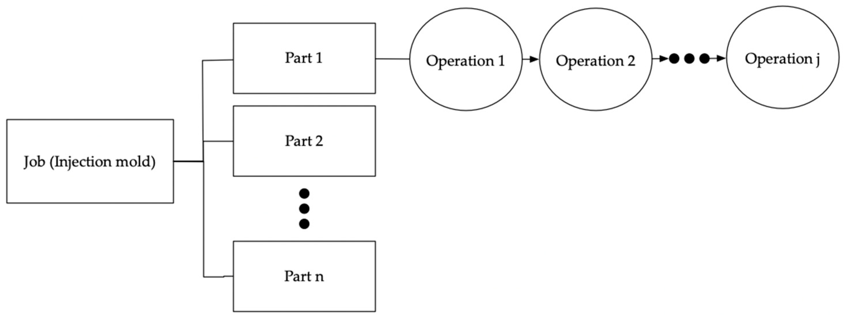
The mold is grouped by size (small, middle, and large) and is named based on the number of parts: a two-plate or a three-plate mold. The mold consists of many parts, and the parts have operations that need to be processed. The mold is completed when the operations of all the parts are finished. Figure 1 shows the configuration of the mold. The processing time of the operations is dependent on the type and size of the mold. In this study, it is assumed that if the size of the mold is large, the operation processing time is longer. For example, if there are operations for large and small molds, respectively, and they are the same, the processing time of the operation for a large mold is longer than the small mold. Additional assumptions are as follows:

• The moving time between the operations is excluded.
• The machines that have the same type are considered to have equal abilities.
• One operation can be processed on a machine at a time.
• The number of operations and parts are known and are not changed until the mold is completed.
• If the machine is idle, the operation of parts that are waiting for assigning is allocated to the spot unless the number of waiting operations is empty.
• The machine is dedicated to certain types of operations.
• When the setup of the machine is changed, the setup time occurs.

3.2. Mathematical Modeling

In this section, a mathematical model is presented for the mold scheduling problem that has been previously described. This model shows the decision-making point with constraints for mold scheduling.

$$\underset{ }{\min }{{\displaystyle \sum }}_i{w}_i{T}_i$$

(1)

Subject to

$$T_i\ge C_i-d_i, \forall i\in ℐ$$

(2)

$${st}_{ipo}\ge {st}_{ip\left(o-1\right)}+{\sum }_k{pt}_{ip\left(o-1\right)}·x_{ip\left(o-1\right)k},\forall i\in ℐ,p\in {𝒫}_i,o\in {𝒪}_p^i,o>1,k\in {ℳ}_{p\left(o-1\right)}^i$$

(3)

$$\begin{array}{c}{st}_{ipo}\ge {st}_{i\prime p\prime o\prime }+{pt}_{i\prime p\prime o\prime }+{su}_{ipoi\prime p\prime o\prime k}-\left(2-x_{ipok}-x_{i\prime p\prime o\prime k}+y_{ipoi\prime p\prime o\prime }\right)·H,\forall i,i\prime \in ℐ,\\ p\in {𝒫}_i,p\prime \in {𝒫}_{i\prime },k\in {ℳ}_p^i\cap {ℳ}_{p\prime }^{i\prime },o\in {𝒪}_p^i,o\prime \in {𝒪}_{p\prime }^{i\prime },|o\ne o\prime \end{array}$$

(4)

$$\begin{array}{c}{st}_{i\prime p\prime o\prime }\ge {st}_{ipo}+{pt}_{ipo}+{su}_{ipoi\prime p\prime o\prime k}-\left(3-x_{ipok}-x_{i\prime p\prime o\prime k}+y_{ipoi\prime p\prime o\prime }\right)·H,\forall i,i\prime \in ℐ,\\ p\in {𝒫}_{i\prime },p\prime \in {𝒫}_i\prime ,k\in {ℳ}_p^i\cap {ℳ}_{p\prime }^{i\prime },o\in {𝒪}_p^i,o\prime \in {𝒪}_{p\prime }^{i\prime },|o\ne o\prime \end{array}$$

(5)

$${st}_{ipo}\ge r_i,\forall i\in ℐ,p\in {𝒫}_i,o\in {𝒪}_p^i,o=1$$

(6)

$$C_{ip}\ge {st}_{ipo}+{\sum }_k{pt}_{ipo}·x_{ipok},\forall i\in ℐ,p\in {𝒫}_i,o\in {𝒪}_p^i,o\in \left|{𝒪}_p^i\right|,k\in {ℳ}_p^i$$

(7)

$$C_i=\underset{p\in {\mathcal{P}}_i}{\max }{C}_{ip},\forall i\in ℐ$$

(8)

$${\sum }_k{x}_{ipok}=1,\forall i\in ℐ,p\in {𝒫}_i,o\in {𝒪}_p^i,k\in {ℳ}_p^i$$

(9)

$$T_i, C_i,s{t}_{ipo}, C_{ip}\ge 0, x_{ipok},y_{ijp{i}^{\prime }{j}^{\prime }{p}^{\prime }}\in \left\{0, 1\right\}$$

(10)

Equation (1) relates to the objective that minimizes the total weighted tardiness of the jobs. Equation (2) calculates the tardiness of each job. Equation (3) ensures the precedence relations between the consecutive operations of a part for the job. Equations (4) and (5) guarantee that the overlapping of the operations on the machine is restrained. Equation (6) means that the job cannot be started before the release time itself. Equations (7) and (8) calculate the completion time of each part of the job and the finished time for the job, respectively. Equation (9) guarantees that only one operation can be processed on a machine.

3.3. Markov Decision Process Framework

For deep RL, the MDP is proposed in this section, which can mathematically model the decision process. In deep RL, the agent observes the state of the environment at a certain time $t$, $s_t$, and an action, $a_t$, which is selected by the policy of the agent among the actions that are given to the environment. The state is changed to the next state, $s_{t+1}$, through the transition probability, and the reward,$r_t$, is received from the environment. The same procedure occurs at every discrete time. In the next section, the state, action, and reward are described, and the transition probability is excluded because it is not necessarily required for deep RL [28,29].

3.3.1. State

In terms of the environment of the mold production scheduling system, the main information is largely divided by two factors: the machine and the job. In this system, the state is meant to be a set of idle machine statuses. Let ${\overline{K}}_t$ be a set of idle machines and $t{y}_{kt}$ denotes the setup type of the machine $k \in {\overline{K}}_t$ at time t. Machines are dedicated to certain operation types, $sy =\left\{1,2,\dots ,SY\right\}$, and additional setup time occurs if a different type of operation is allocated to the machine that already has the setup type.

For job information, let ${\overline{\mathcal{O}}}_t^k$ be a set of waiting operations at time $t$ for machine $k$ and $S{O}_t^{sy}$ is the sum of the operations that have operation type $sy$ in ${\overline{\mathcal{O}}}_t^k$. As mentioned in Section 2.2, the job has the weight $jw =\left\{1,2,\dots ,JW\right\}$ and let $O{W}_t^{jw}$ be the sum of the operations that have $jw$ at time $t$. Based on the explanation above, the state of each machine $k$ at time $t$,$s_t^k$, is expressed as follows.

$$s_t^k= \left\{t{y}_{kt}, \left( \frac{O{W}_t^1}{\left|{\overline{\mathcal{O}}}_t^k\right|}, \frac{O{W}_t^2}{\left|{\overline{\mathcal{O}}}_t^k\right|},\dots ,\frac{O{W}_t^{JW}}{\left|{\overline{\mathcal{O}}}_t^k\right|}\right),\left( \frac{S{O}_t^1}{\left|{\overline{\mathcal{O}}}_t^k\right|}, \frac{S{O}_t^2}{\left|{\overline{\mathcal{O}}}_t^k\right|},\dots ,\frac{S{O}_t^{SY}}{\left|{\overline{\mathcal{O}}}_t^k\right|}\right) \right\}, \forall k, t$$

(11)

In Equation (11), by dividing the total number of operations, $\left|{\overline{\mathcal{O}}}_t^k\right|$, the state vector is standardized as a set of vector numbers that are expressed in the range of [0, 1]. By doing this, the agent is able to visit all the states [23]. Finally, $s_t$ can be expressed as follows.

$$s_t= \left\{s_t^1 ,s_t^2,\dots ,s_t^K\right\}, \forall t$$

(12)

3.3.2. Action

The action refers to the selection of the operation for assigning an idle machine $k$. Hence, the candidates of the action, which is the action space, is the total number of waiting operations for machine $k$. Equation (13) shows the action space for $s_t^k$.

$$a_t^k\in \left\{{\overline{\mathcal{O}}}_t^k\right\}, \forall k, t$$

(13)

Based on Equation (13), $a_t$ can be described as follows.

$$a_t= \left\{a_t^1,a_t^2,\dots ,a_t^K\right\}, \forall t$$

(14)

3.3.3. Reward

The reward is meant to be the objective of the mold production system, which minimizes the total weighted tardiness. To calculate the tardiness of the job, the completion time is required, which is difficult to calculate at the decision point. In addition, even if the completion time of the job is expected at the decision point, it is important to consider the possibility that the job might be finished earlier or later than the expected time owing to other jobs’ schedules.

In this study, the processing time of the operation that is selected as the action is regarded as the reward. At the decision point, the processing time of the operation is not known; hence, the decision is made by using the average processing time. By multiplying the weight of the operation of the job, the weight of the job is reflected in the reward.

If the processing time of the last operation is long, this may have the impact that the tardiness is larger. The reward formulation considers that it prevents larger tardiness by the long processing time of the last operation and selects the operation that belongs to the job that has a high weight first.

From the above, the reward consequential to the action for each machine is formulated in Equation (15), and $r_t$ is expressed in Equation (16).

$$r_t^k=w_i·p_{ipo},$$

(15)

$$r_t=\left\{r_t^1,r_t^2,\dots ,r_t^K\right\}, \forall t$$

(16)

3.4. Deep RL for the Mold Production Scheduling System

Based on the aforementioned details, in this study, the agents and the environment are structured and interact, as illustrated in Figure 2. There are as many agents as the number of machines. Once a machine is idle, the agent corresponding to the machine observes the machine state. When observing, the setup type of the machine and the waiting operations to be allocated for the machine are considered. Then, the agent selects the operation while waiting, according to the policy of the neural network, which is the brain of the agents. After taking the action, the agent obtains the reward from the environment. As suggested in [30], while each agent acts in a decentralized fashion, the neural network is shared to take advantage of centralized learning. Therefore, when the elements in the environment change, for example, the number of machines change, the DQN does not need to be retrained.

Algorithm 1 shows the mold scheduling procedure that is based on the DQN algorithm for training. At time $t$, when ${\overline{\mathcal{K}}}_t$ and ${\overline{\mathcal{O}}}_t^k$ exist at the same time, scheduling is implemented on the basis of the DQN algorithm until one of them is empty. When the agent selects the action, there are two ways to achieve this: random selection and $Q$-value selection. Random selection is ε greedy and the procedure is as follows. A random variable is generated, and if it is less than the ε value, then the action is selected randomly. Otherwise, the action is chosen following the maximum $Q$-value. To calculate the $Q$-value of each action, the operation’s average processing time, the type of the operation, and the staying time of the job that the operation belongs to are considered.

Algorithm 1. DQN for mold scheduling

Input: scheduling problem

Output: Parameters θ of a $Q$-Network

1: Initialize replay memory $U$

2: Initialize $Q$-Network with weights $\theta$

3: Initialize target network $Q$ with weights ${\theta }^{-}$

4: for ep = 1, T do

5:  Get ${\overline{\mathcal{K}}}_t$ and ${\overline{O}}_t^k$

6:  if ${\overline{\mathcal{K}}}_t\ne \varnothing$ and ${\overline{\mathcal{O}}}_t^k\ne \varnothing$ then

7:   repeat

8:    Observe $s_t$

9:    Select a random action $a_t$ with probability ε greedy policy.

Otherwise, $a_t=\underset{a}{\max }Q\left(s_t, a;\theta \right)$

10:   Execute ${\mathrm{a}}_{\mathrm{t}}$ (select $o\in {\overline{O}}_{kt}$, which is assigned to machine $k$)

11:   Observe $s_{t+1}$, and $r_t$ is given to the agent

12:   Save transition $\left(s_t, a_t,r_t,s_{t+1}\right)$ in $U$

13:   ${\overline{\mathcal{K}}}_t\leftarrow {\overline{\mathcal{K}}}_t\backslash \left\{k\right\}$, ${\overline{O}}_t^k\leftarrow {\overline{O}}_t^k\backslash \left\{o \right\}$

14:   until ${\overline{\mathcal{K}}}_t=\varnothing$ or ${\overline{\mathcal{O}}}_t^k=\varnothing$

15:  end if

16:   if $\left|U\right|\ge L$ then

17:   Sampling random minibatch $\left(s_q, a_q,r_q,s_{q+1}\right)$ from $U$

18:   Calculate loss

19:   Perform a gradient decent regarding weights $\theta$

20:  end if

21: if $\left|U\right|\ge L$ and $ep \% N=0$

22:  update ${\theta }^{-}=\theta$

23: end if

24: end for

The waiting time is calculated by the current time minus the release time of the job. Algorithm 2 explains the procedure for selecting the action. The transition is stored in the memory replay $U$. When the transitions are more than half of the size of $U$, the loss is calculated with the random minibatch from $U$. Lastly, in every $N$ episode after calculating the loss, the target weight is updated. Figure 3 shows the framework for the steps of the proposed method.

Algorithm 2. Action selection

1: random value $\leftarrow$ random ( ):

2:  if random value $\le ϵ$ then

3:    action $\leftarrow$ random $\left({\overline{\mathcal{O}}}_t^k\right)$

4:  else

5:    action $\leftarrow$ $maxQ\left(s_t^k,{\overline{\mathcal{O}}}_t^k\right)$

6:  end if

The proposed scheduling method consists of training and testing phases. In the training phase, the same scheduling problem is solved iteratively, and the scheduling problems with the other condition are solved in the testing phase. Figure 4 shows the framework of the DQN training for this study. After training, in the testing phase, the proposed method with the trained weight of the $Q$-network is tested to compare the other dispatching rules in the new scheduling problems to check the performance.

4. Experimental Results

This section describes the results of the proposed method for the mold scheduling problem and it provides a comparison of the dispatching rules. The proposed method was coded in Python with the Keras application programming interface and tested on a 3.2 GHz Intel i7 with 16 GB of RAM. The neural network that was used for the method is fully connected, and there are four hidden layers. Each node has 64, 32, 16, and 8 layers, respectively, and the leaky rectified linear unit is used as an activation function for all the layers. For the testing phase, the hyperparameters that are used for the test are listed in

Table 1. Hyperparameters.

Hyperparameter	Value
Learning rate	0.001
Discount factor $\gamma$	0.9
Epsilon to select action randomly $ϵ$	0.1
Update target point $N$	10
Minimum training point $L$	1000
Size of memory $U$	20,000
Iteration	3000
Batch size	64
Optimizer	RMSprop

.

After applying the hyperparameters, the method’s performance is influenced; however, the optimal value of the hyperparameters is difficult to determine because of the large search space. In this study, a random search [31] was conducted to find the best value.

For the testing data, the data were received from a small Korean company that made molds that customers order. Some of the missing information was gained from the staff that worked for the company. The molds were divided into three categories: small, medium, and large. The number of parts that are needed for making the molds is dependent on the order of the customers and their size. In this study, the main parts, the main and base cavity, and the core, which are the most critical parts, were considered. Depending on the size, additional parts were considered. According to the size, the number of small, medium, and large parts is three, four, and five. In addition, the processing time of the operations is dependent on the size. The increasing ratio of the average processing time for small, medium, and large is 1, 1.3, and 1.6, respectively. The operations of each part are different, and nine patterns were extracted from them.

Table 2. Operation patterns.

Pattern	Description
1	A → C → D
2	A → C → D →E
3	A → C → D → B → G → E
4	H → C → D → E
5	A → C → B
6	A → B → C → F → D → E
7	A → C
8	A → F → C → E
9	A → F → D → E

→: Operational sequence direction.

shows the operating patterns. The arrow sign is meant for the direction of the operations, and the next operation can be commenced when the predecessor operation is finished.

The due date of the jobs is 1.3 times the average sum of the processing time of the operations, and the weight $w_i$ is assigned in accordance to the size: 1 for small, 2 for medium, and 3 for large. To compare the performance of the proposed method, four dispatching rules were designed. In order to determine whether an operation should be allocated to an idle machine, two steps need to be performed.

As the job contains parts and the parts have operations, one of the parts for the available jobs can be determined. In other words, (1) a job is selected among the available jobs, and (2) the operation of the available parts for the job is chosen. Because the objective of the problem is to minimize the total weighted tardiness, they consider the earliest due date (EDD) rule for the job selection. The EDD rule selects the shortest remaining time for the job and it is expressed as $\underset{i\in {\overline{ℐ}}_t}{\min }\left\{d_i-t\right\}$ where ${\overline{ℐ}}_t$ is a set of available jobs at time $t$. Three out of four dispatching rules (ES, EL, EC) use the EDD rule for the job selection. The last rule (WEL) considers the waiting time as well as the EDD, which is $\underset{i\in {\overline{ℐ}}_t}{\min }\left\{\left(wa·\left(d_i-t\right)+\left(1-wa\right)·\left(t-r_i\right)\right)\right\}$ where $wa$ is the weight for the EDD and the waiting time is set to 0.8.

Next, the second step for the four dispatching rules is explained. The first rule (ES) considers the shortest remaining average processing time. The operation of the part that is the smallest sum of the remaining average processing times for the available parts of the selected job is selected. Let ${\mathcal{O}}_{pt}^i$ be a set of operations for part $p$ of job $i$ at time $t$ and the second decision for the first rule can be expressed as $\underset{p\in {\mathcal{P}}_i}{\min }\left\{{\sum }_{o=1}^{\left|{\mathcal{O}}_{pt}^i\right|}{p}_{ipo}\right\}$. The second rule (EL) is used to contemplate the longest average processing time. The operation of the part that is the largest sum of the remaining average processing times among the available parts for the selected job is chosen, $\underset{p\in {\mathcal{P}}_i}{\max }\left\{{\sum }_{o=1}^{\left|{\mathcal{O}}_{pt}^i\right|}{p}_{ipo}\right\}$. The critical ratio is considered in the third rule (EC) for the part selection. It selects the operation of the part that has the smallest value, which is calculated using the due date of the job. This is followed by performing a subtraction from the current time, and then it is divided by the sum of the remaining average processing times for the job’s part, $\underset{p\in {\mathcal{P}}_i}{\min }\left\{\frac{\left(d_i-t\right)}{{\sum }_{o=1}^{\left|{\mathcal{O}}_{pt}^i\right|}{p}_{ipo}}\right\}$.In the last rule (WEL), the method of selecting the part for the operation is the same as that of EL.

Table 3. Composite dispatching rules.

Dispatching Rule	Job Selection	Part Selection
Earliest due date with the shortest remaining average processing time (ES)	$\underset{i\in {\overline{ℐ}}_t}{\min }\left\{\left(d_i-t\right)\right\}$	$\underset{p\in {\mathcal{P}}_i}{\min }\left\{{\sum }_{o=1}^{\left|{\mathcal{O}}_{pt}^i\right|}{p}_{ipo}\right\}$
Earliest due date with the longest remaining average processing time (EL)		$\underset{p\in {\mathcal{P}}_i}{\max }\left\{{\sum }_{o=1}^{\left|{\mathcal{O}}_{pt}^i\right|}{p}_{ipo}\right\}$
Earliest due date with the critical ratio (EC)		$\underset{p\in {\mathcal{P}}_i}{\min }\left\{\frac{\left(d_i-t\right)}{{\sum }_{o=1}^{\left|{\mathcal{O}}_{pt}^i\right|}{p}_{ipo}}\right\}$
Earliest due date and waiting time with the longest remaining average processing time (WEL)	$\underset{i\in {\overline{ℐ}}_t}{\min }\left\{\left(wa·\left(d_i-t\right)+\left(1-wa\right)·\left(t-r_i\right)\right)\right\}$	$\underset{p\in {\mathcal{P}}_i}{\max }\left\{{\sum }_{o=1}^{\left|{\mathcal{O}}_{pt}^i\right|}{p}_{ipo}\right\}$

shows the composite dispatching rules at a glance.

To evaluate the performance of the proposed method, five scenarios are assumed with different occurrence ratios of the job’s size. As the size of the job takes up a large proportion of the objective function because the larger size of the job can have more operations, each scenario has a different occurrence ratio, which is shown in

Table 4. Occurrence ratio for the size of the mold.

Scenario	Small	Medium	Large
1	0.3	0.6	1
2	0.5	0.8	1
3	0.2	0.7	1
4	0.3	0.5	1
5	0.1	0.2	1

as a cumulative value.

In this study, four types of machines were considered. Each type of machine is dedicated to certain operations as follows: type 1 for operations A and C, type 2 for operations B and D, type 3 for operations E and F, and type 4 for operations G and H. There are 11 machines and $\left\{3, 5, 2, 2\right\}$ from types 1 to 4.

For the training phase, with an instance of 10 jobs in scenario 1, the neural network was trained for 3000 episodes. During the training, the selection of an operation was based on the average processing time, and the actual processing time was the same for all the episodes. Therefore, the neural network can learn about the static environment first. Figure 5 shows the results of the total weighted tardiness that was obtained by the DQN in 3000 episodes. As shown, the curve of the graph gradually decreases with an increase in the episode, which indicates that the proposed DQN learned the proper policy for the scheduling problem.

The total number of jobs in the testing phase was 10, 30, 50, and 70 for each scenario; thus, a total of 20 cases were used for testing the proposed method. Each case was tested with 100 independent instances, and the total number of operations that had to be processed for each job was approximately 150, 500, 800, and 1000. The trained $Q$ network was selected for testing during the 2633rd episode, which showed the best performance during the episodes. The results are represented by the average values for 100 instances, which are shown in

Table 5. Results for the mean of the total weighted tardiness.

Jobs	Rule	Scenario 1 $\left({10}^2\right)$	Scenario 2 $\left({10}^2\right)$	Scenario 3 $\left({10}^2\right)$	Scenario 4 $\left({10}^2\right)$	Scenario 5 $\left({10}^2\right)$
10	Deep RL	8.7	7.1	10.1	9.9	14.3
	ES	40.9	30.9	43.3	48.7	69.8
	EL	32.9	25.2	35.3	37.1	55.8
	EC	38.0	29.3	40.9	42.8	60.7
	WEL	22.7	18.2	24.6	26.2	35.3
30	Deep RL	260.2	188.7	279.2	284.9	438.0
	ES	570.3	434.4	611.1	650.7	929.4
	EL	518.3	394.9	565.0	592.2	838.8
	EC	519.9	398.1	560.1	583.4	864.5
	WEL	469.1	363.5	494.4	535.1	720.5
50	Deep RL	863.2	648.2	945.9	978.1	1391.5
	ES	1595.6	1327.3	1831.4	1984.6	2758.3
	EL	1597.9	1271.7	1734.6	1880.5	2595.0
	EC	1595.6	1243.6	1755.7	1856.0	2586.9
	WEL	1428.2	1142.8	1546.7	1689.5	2266.7
70	Deep RL	1797.7	1295.5	1953.3	2042.5	2875.6
	ES	3372.4	2538.9	3652.1	3863.5	5479.5
	EL	3233.3	2423.5	3493.9	3700.1	5214.2
	EC	3304.3	2541.7	3601.4	3754.7	5382.6
	WEL	2991.4	2271.6	3224.4	3415.0	4707.1

. In all the scenarios, the performance of deep RL for minimizing the total weighted tardiness outperformed the other dispatching rules. Even in an extreme situation, such as scenario 5, the deep RL showed a better performance than the other dispatching rules, and it was observed that the deep RL worked to schedule the operations in harsh conditions. As the number of jobs increased, the standard deviation of the deep RL was larger than the other rules, as shown in Figure 6.

Specifically, in the case of 50 and 70 jobs, the standard deviation of the deep RL was largest, which showed that there was a large difference between the best and the worst performance. Another interesting thing is that WEL had a better performance than the rest of the rules, because the rule considered the combination of the waiting time and the due date of the job. This means that the waiting time may be necessary to prevent certain jobs from waiting for too long.

Figure 7 shows the results of the total weighted tardiness for each instance for 30 jobs in scenario 1 and the average, minimum, and maximum of the total weighted tardiness in the box plot. The orange bar in the rectangular box indicates the median value, the green dot is the mean value, and the asterisk in blue is an outlier. As shown in Figure 7, in many instances, it is difficult to determine the superiority of the inferior performance of the dispatching rules. However, deep RL showed a stable performance in most instances. This observation shows that deep RL is larger than the other dispatching rules depending on the uncertainty of the processing time.

5. Discussion

In a manufacturing environment, it is difficult to make a decision to schedule jobs under a dynamic situation, and it is important to provide the decision-maker with a certain rule or policy to achieve efficient scheduling. In a variety of studies, rule-based methods have been employed for scheduling jobs; however, this method has some disadvantages. One of the disadvantages is that a single rule cannot outperform the other rules for different shop configurations [32]. The results that are presented in this study show that the deep RL method for scheduling jobs to minimize the total weighted tardiness can perform better than the other suggested rules in diverse situations. In most instances, the performance of deep RL was higher than the other rules, which is stable in a dynamic situation. In all the scenarios, the processing time was not the same, which generates different processing times. The information known before the scheduling jobs was the average processing time and the rules that were selected to consider it. In the situation that the processing time was not static, deep RL had a robust performance. Likewise, in the practical manufacturing environment, the exact processing time cannot be expected and the change in the number of machines occurs frequently due to machine break, failure, and so forth. In the situation, the proposed method is able to show better performance and provide a robust scheduling policy.

To reduce the complexity of the state, a novel definition state is proposed to recognize the environment. In addition, generally, the reward is equivalent to the objective function. However, it is highly difficult to anticipate the tardiness because the mold product consists of several parts and the parts have operations to be processed on dedicated machines. To complete the mold product, the operations of all parts are finished. In addition, as the operations of the parts of a mold product are affected by machine status and other parts of other products, selecting the operation of a part from the waiting parts to be processed on an idle machine by calculating the tardiness in the middle of the manufacturing the mold is complex and difficult. Even if the expected tardiness is calculated, the accuracy of the calculation may not be guaranteed due to the dynamic environment. In this study, the reward for considering the objective that minimizes the total weighted tardiness is designed in the view of the processing time of the operation. The agent tends to maximize the sum of the rewards and, the processing time of the operation and the weight of the product that the operation belongs to are considered to the reward. This is equivalent to that the operation that has the longest processing time is allocated first among others in consideration of the weight of the product that includes the operation. By doing this, although this is not related to the tardiness of the product directly, it prevents the tardiness is larger by the last operation of the product.

To apply the proposed method practically, the manufacturing scheduling system is required with computer support for solving scheduling problems. Basically, all data is collected from all machines and the information of customers’ orders is stored in the database system. Using historical data, the neural network is learned with the proposed state, action, and reward. After enough learning, the neural network is used to schedule the operations on idle machines. At that time, the transmission between the neural network and the idle machines should be possible. Depending on manufacturing sites, the instruction to select the operation from the neural network is given to workers in front of machines or machines directly. In addition, learning the neural network that is the weight needs to be done periodically to accommodate the change of the manufacturing environment, as the weight is a key factor that decides the action based on the state. When using the suggested scheduling model, the assumptions for the model are addressed to fit the manufacturing field. For example, if the distance between machines is far, the moving time should be considered to add a new decision variable. Furthermore, the assumption that the same type of machine has the same ability is handled as the actual ability. For instance, average processing time may be different between the same type of machines so that the ability is considered by the field data.

The proposed algorithm provides benefits in the view of the management for the manufacturing process. As the algorithm is based on the learning with historical data, the proposed algorithm can confront manufacturing processes flexibly in an unpredictable situation so that the cumbersome works can be reduced such as reconfiguration of scheduling policy due to unexpected situations. In addition, even if new processes are added, the algorithm is updated through simulation before applying to the production system so that the efficiency of the production is sustained.

In the proposed method, the $Q$-networks were trained with a small-scale problem, and then the trained $Q$-network was used for large-scale problems. As a result, the deep RL showed a good performance in comparison to the other rules without retraining, which shows the robustness of the trained $Q$-network. Additionally, in the proposed method, the centralized neural network is designed, so that the neural network is not needed to retrain when the number of the machine is changed.

However, when the type of operations, machines, and the sequence of the operations are changed or are added, the $Q$-network needs to be retrained, which is one of the limitations of this study. Another limitation is that the model has some assumptions that do not embrace all the factors in manufacturing situations. For example, the method of manufacturing molds is different from the specification of what customers order. To embrace this, the order of the customers was largely divided by the size of the mold: small, medium, and large. In addition, all the processes are not included, but the core processes are considered to represent mold manufacturing. In this study, diverse machines were not considered, and it is assumed that the machines have the same performance. In the real world, the performance can differ depending on the machine year. However, the difference between the machines was included in the processing time as the processing time of the operations was not the same for every instance.

In terms of future research, a state is needed to develop $Q$-networks that are not necessary for retraining, even though operation types, machine types, and so forth are changed. In addition, more uncertain factors, such as the breakdown of machines, can be considered. It can be extended as a multi-objective, such as minimizing the makespan and tardiness as they are conflicted. As another future research, the performance of the proposed algorithm can be compared with other heuristic algorithms that were presented in other studies [33].

6. Conclusions

In Industry 4.0, as manufacturing firms consider technical issues for sustainability as well as economic, environmental, and social issues, they try to enhance the production efficiency and meet customers’ demand with the technical introduction to the manufacturing. To fulfill the firms’ exertion, enhancing the agility of manufacturing is key. Because the manufacturing environment is getting dynamic due to an increase in the number of products to be produced, not responding to the environment with agility causes customers’ dissatisfaction and has a negative influence on the companies’ competitiveness in the market as a result. Therefore, intelligent systems have been required to cope with the dynamic environment for complex production systems to enhance sustainability.

In complex production systems, scheduling is a core process that can increase profits and reduce costs. Manufacturing molds consist of complex production systems since many parts are combined and the specification of each mold is different. Moreover, the parts have different processes, and those factors induce the dynamic manufacturing environment. Due to the complexity and the dynamic environment, the importance of scheduling for mold manufacturing has emerged and sustainable and intelligent scheduling has been required to handle them with agility. However, few studies have been conducted on scheduling in mold manufacturing. In addition, the literature has proposed heuristic rules that are intractable in the real world. To address the complexity and the dynamic environment as well as practicality, in this study, deep RL was designed for mold scheduling problems. Before applying deep RL, a mathematical model was developed for the mold scheduling problem, and the MDP was presented for the objective of minimizing the total weighted tardiness. The algorithm of deep RL, DQN, was used to find the optimal scheduling policy for the mold scheduling problem.

To evaluate the performance of deep RL, some dispatching rules were suggested as a comparison with deep RL. As a result, deep RL outperformed the other dispatching rules under diverse scenarios. In the case that has large operations and a large number of high-weighted jobs, deep RL showed a lower total weighted tardiness than the others. Moreover, even in the situations in which the processing time for each instance was not deterministic, the proposed method assures good performance in a dynamic situation.