How Does Heterogeneity Affect Freeway Safety? A Simulation-Based Exploration Considering Sustainable Intelligent Connected Vehicles

Abstract

Intelligent connected vehicles (ICVs) are recognized as a new sustainable transportation mode, which could be promising for reducing crashes. However, the mixed traffic consisting of manually driven vehicles and ICVs may negatively affect road safety due to individual heterogeneity. This study investigated heterogeneity effects on freeway safety-based simulation experiments. Two types of vehicle dynamic models were employed to depict dynamic behaviors of manually driven vehicles and adaptive cruise control (ACC) vehicles (a simplified version of ICVs), respectively. Real vehicle trajectories were utilized to calibrate model parameters based on genetic algorithms. Surrogate safety measures were applied to establish the relationship between vehicle behaviors and longitudinal collision risks. Simulation results indicate that the heterogeneity has negative effects on longitudinal safety. With the higher degree of heterogeneity, longitudinal collision risks are increased. Compared to traffic flow consisting of human drivers only, mixed traffic flow may be more dangerous when the market penetration rate of ACC is low, since the ACC system can be recognized as a new source of individual heterogeneity. Findings of this study show that necessary countermeasures should be developed to improve safety for mixed traffic flow from the perspective of transportation safety planning in the near future.

1. Introduction

Traffic crashes cause grave losses of life and property all over the world. The rear-end crash is the most frequently occurring type, resulting in approximately 34% of the total reported crashes in the United States [1]. The proportion is also high in China, which occupies about 40% of all highway crashes [2]. Therefore, considerable studies have been conducted to reduce rear-end crashes [3,4,5,6].

Previously, most efforts have been taken to develop a variety of crash prediction models to investigate contributing factors of rear-end crashes. In general, reported historical crash data are exploited and various factors, such as traffic volume, speed, weather, vehicle type and others, are examined in various models [7,8,9,10]. There are also some non-parametric methods based on machine learning models proposed for rear-end crash analysis [11,12].

Among the above studies, dozens of random effect and random parameter models have been developed to capture unobserved heterogeneity [8,13,14,15,16], but these models take into account heterogeneity mostly from crash data level instead of individual behavior level. The individual heterogeneity is caused by differences among drivers’ age, gender, driving experience, preference and so on, which is a microscopic characteristic. It has been demonstrated in previous studies that these factors could result in heterogeneity and cause significant effects [17]. Although individual heterogeneity of human drivers plays a critical role, there is a lack of exploitation.

On the other hand, with the advancement of wireless communication and automation technologies, intelligent connected vehicles (ICVs) are recognized as a new sustainable transportation mode, which could be promising for reducing crashes [6,18,19,20,21,22,23,24]. The ICVs include two aspects, i.e., the connected vehicle and the autonomous vehicle that focuses on the communication and automation technologies, respectively. A large amount of prior research has demonstrated the potential of ICVs to enhance safety, but most of them consider the ideal scenarios with high market penetration rates of ICVs and take into no account the individual heterogeneity. The ICVs can be recognized as a unique individual, which has different characteristics and maneuvers from manually driven vehicles. Therefore, at the early state of ICVs’ popularization, the market penetration rate is still very low, and the ICVs become a new source of individual heterogeneity in mixed traffic flow. The safety effect of the heterogeneous mixed traffic flow also lacks an in-depth analysis.

The above research gaps motivate the present study to investigate influences of the individual heterogeneity on rear-end collision risks, i.e., the longitudinal safety, based on simulation experiments. The individual heterogeneity effects are explored in two perspectives: (1) how does human drivers’ heterogeneity affect longitudinal safety on traffic flow consisting of only manually driven vehicles; and (2) how do adaptive cruise control (ACC) vehicles (a simplified version of ICVs) impact the mixed traffic flow consisting of both manually driven and ACC vehicles. Results of this study could provide insights towards influences of individual heterogeneity on longitudinal safety and improve freeway safety for mixed traffic flow from the perspective of transportation safety planning in the near future.

2. Methods

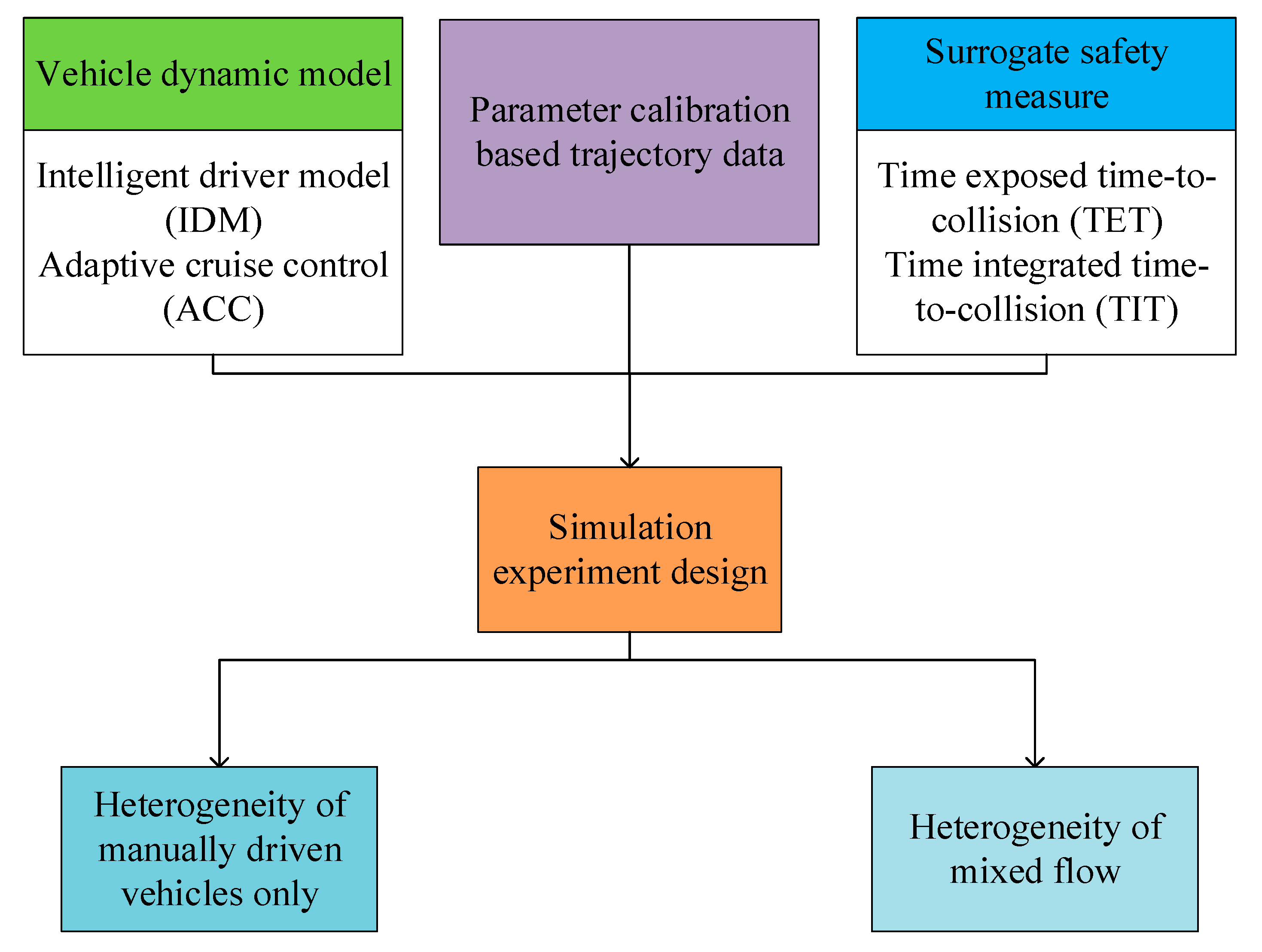
2.1. Research Framework

An overview of the research framework is displayed in Figure 1. Two types of vehicle dynamic models were applied to depict longitudinal car-following behaviors, i.e., the intelligent driver model (IDM) for manually driven vehicles and the ACC model for ACC vehicles, respectively. Note that, a large number of car-following models have been previously proposed, including stimulus–response models, desired measures models and psycho-physical models. The IDM belongs to the desired measures model, which can take the desired space, headway and speed into account and is one of the most widely employed car-following models.

The real trajectory data were extracted to calibrate model parameters. Two surrogate safety measures derived from the time-to-collision (TTC) index were applied for longitudinal safety evaluations, including the time exposed time-to-collision (TET) and time integrated time-to collision (TIT). With vehicle dynamic models and safety measures, extensive simulation experiments were designed and conducted to examine influences of heterogeneity on longitudinal safety. Two different heterogeneity scenarios were investigated in the present study. One is the individual heterogeneity in a traffic stream consisting of only manually driven vehicles, and the other is in the mixed traffic flow consisting of manually driven vehicles and ACC vehicles. A microscopic simulation platform was developed based on MATLAB 2019b software, integrating the above vehicle dynamic models, surrogate safety measures and calibrated parameters to investigate the aforementioned heterogeneity.

2.2. Vehicle Dynamic Models

2.2.1. Human Driver Model

The car-following models were employed to describe longitudinal dynamics of manually driven vehicles in this study. The intelligent driver model (IDM) is one of the most commonly used models [22,25,26,27], which calculates vehicle dynamic accelerations using desired speed and gap distance and can be expressed as follows:

$$a={\alpha }_m[1-{\left(\frac{v}{v_0}\right)}^4-{\left(\frac{s^{*}}{s}\right)}^2]$$

(1)

$$s^{*}=s_0+\max [0,vT+\frac{v\Delta v}{2\sqrt{{\alpha }_m\beta }}]$$

(2)

where $a$ denotes the acceleration of subject vehicle; ${\alpha }_m$ denotes the maximum acceleration; $v$ and $v_0$ are the speed and the desired speed of subject vehicle, respectively; $s$ is the gap distance between the subject and preceding vehicles; $s_0$ denotes the minimum gap distance at standstill; $T$ is the safe time gap; $\Delta v$ denotes the speed difference between subject and preceding vehicles; and $\beta$ is the desired deceleration.

With the dynamic accelerations, vehicles’ speeds and positions can be calculated:

$$v=v_{prev}+a\Delta t$$

(3)

$$x=x_{prev}+v\Delta t+a{\left(\Delta t\right)}^2/2$$

(4)

where $x_{prev}$ and $v_{prev}$ denote the position and speed of the subject vehicle in the previous time step; and $\Delta t$ is the simulation time step and is set as 0.1 s.

2.2.2. ACC Models

The ACC model proposed by the California Partners for Advanced Transit and Highways (PATH) was employed in this study. The PATH ACC model was derived from real vehicle tests and reveals performances of the current ACC systems [28,29,30]. Similar to conventional car-following models, the ACC model can be expressed as follows:

$$a_i=k_1\left(x_{i-1}-x_i-t_{hw}{v}_i-L_{i-1}\right)+k_2\left(v_{i-1}-v_i\right)$$

(5)

where $a_i$ denotes the acceleration of the subject ACC vehicle; $x_{i-1}$ and $v_{i-1}$ denote the position and speed of preceding vehicle, respectively; $x_i$ and $v_i$ represent the position and speed of subject vehicle, respectively; $t_{hw}$ denotes the time gap of ACC vehicles; $L_{i-1}$ denotes the preceding vehicle length; and $k_1$, $k_2$ represent the model coefficients. With the dynamic accelerations, vehicles’ speeds and positions can also be calculated by Equations (3) and (4).

2.3. Trajectory Data Collection and Parameter Calibration

2.3.1. Trajectory Data Collection

In this study, real vehicle trajectory data were utilized for model parameter calibrations. Vehicle trajectory is a new type of traffic data, promoted by the advancement of traffic video surveillances and processing. Generally, trajectory data include time, vehicles’ longitudinal and lateral positions, velocities, accelerations, preceding and following vehicle ID and other information at each second or sub-second. This study applied trajectories collected by the Federal Highway Administration’s Next Generation Simulation (NGSIM) project [31]. The NGSIM data were collected via video cameras fixed on tall buildings and extracted automatically based on a special software with 10 frames of data per second.

The dataset utilized in this study was collected from the Interstate 80 (I-80) in Emeryville, California from 5:00 p.m. to 5:15 p.m. on 13 April 2005. The studied freeway site has six lanes in one direction with the length of approximately 1650 feet. The average flow of the site was 7124 vph and the time mean speed was only 18.62 mph, indicating a typical congested condition. The congested traffic condition generated considerable car-following vehicle pairs that were suitable for longitudinal safety analysis. The criterion of data extraction is that vehicles have to maintain the stable car-following state without any lane-changing behaviors. After the careful selection, a total of 513 car-following pairs with 195,029 frames of data were extracted from the original dataset and employed for parameter calibrations. All the data were smoothed before calibrations to reduce the impact of data noises.

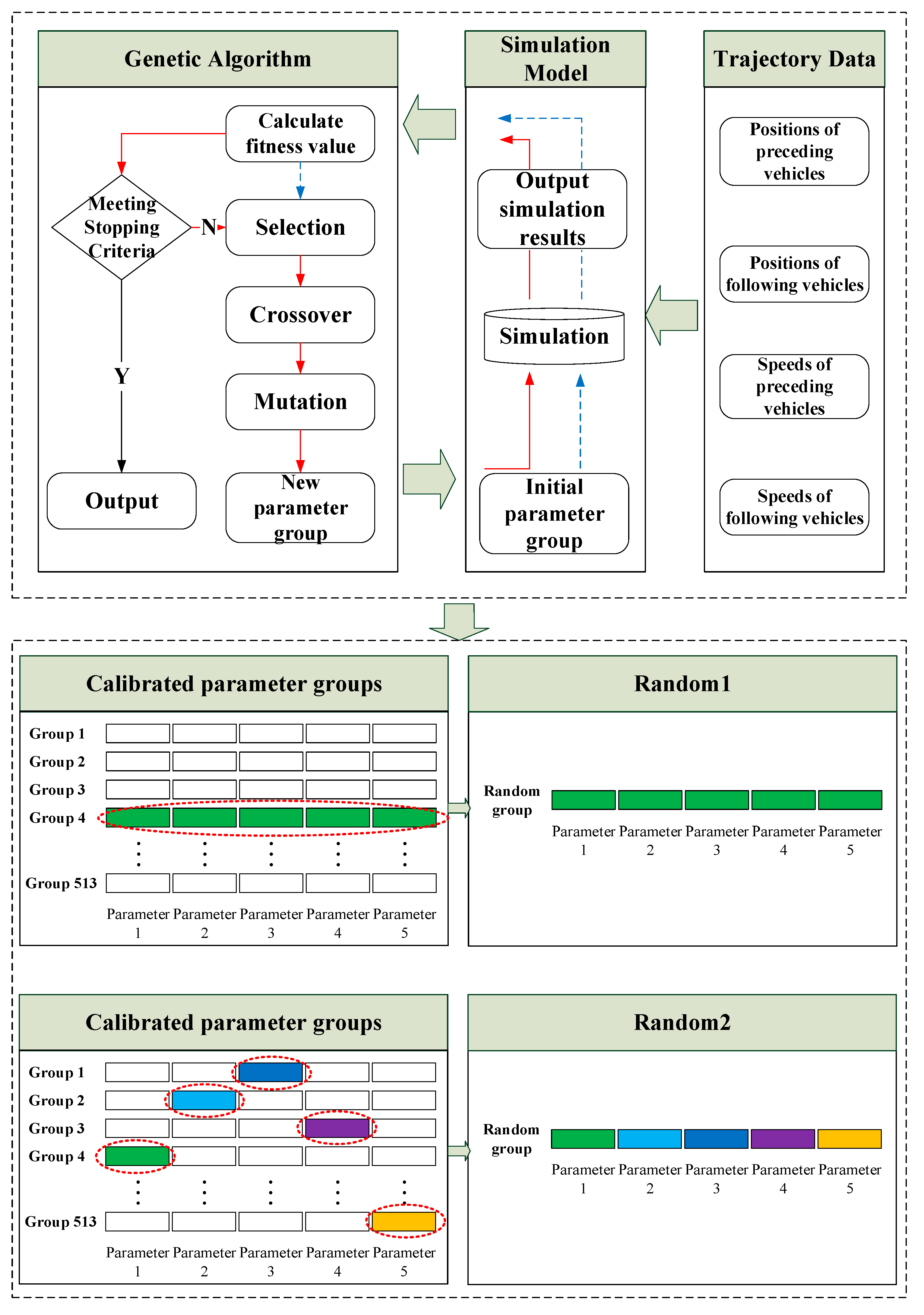
2.3.2. Parameter Calibration

As mentioned in the framework, there are two types of vehicle models, the IDM for manually driven vehicles and the ACC model for ACC vehicles. Previously, research has utilized reasonably fixed parameter values for the IDM to simulate car-following vehicles. These fixed parameters are able to capture traffic flow phenomenon, such as stop-and-go waves and flow breakdown but are not realistic for safety analysis. In practice, individual heterogeneity undoubtedly exists across different drivers, therefore the parameter values are supposed to be distinct for each driver.

Therefore, for the IDM, we employed the commonly used parameter values as the benchmark for assessment, which are denoted as the fixed parameters. The heterogeneous values were calibrated by real vehicle trajectory data and generated based on two different randomization methods. The parameters in the IDM included $s_0$, $T$, ${\alpha }_m$, $\beta$, and $v_0$, and their fixed values were set according to previous studies as follows: the minimum distance at standstill $s_0$ was set as 0.3 m; the time gap $T$ was set as 1.19 s; the maximum acceleration ${\alpha }_m$ and the desired deceleration $\beta$ were set as 1.52 m/s⁻² and 3 m/s⁻², respectively; $v_0$ denoted the maximum desire speed and was set as 33.3 m/s [28,29,32,33].

With respect to heterogeneous parameter values in the IDM, the real-world trajectory data of manually driven vehicles from the NGSIM dataset were employed and the genetic algorithm was developed for parameter calibrations. The core aim of the parameter calibration is to minimize the errors between real trajectory data and the simulated data. The objective function of the minimization is as follows:

$${\epsilon }_m\left(\theta \right)=\frac{\sqrt{{\sum }_t{[x_m\left(t\right)-x_r\left(t\right)]}^2}}{\sqrt{{\sum }_t{[x_r\left(t\right)]}^2}}+\frac{\sqrt{{\sum }_t{[v_m\left(t\right)-v_r\left(t\right)]}^2}}{\sqrt{{\sum }_t{[v_r\left(t\right)]}^2}}$$

(6)

$${\theta }^{*}=\arg \min {\epsilon }_m\left(\theta \right)$$

(7)

where $x_m\left(t\right)$ and $x_r\left(t\right)$ are simulated and real positions at time $t$, respectively; $v_m\left(t\right)$ and $v_r\left(t\right)$ are simulated and real speeds at time $t$, respectively; $\theta$ is used to represent for all five parameters in the IDM and ${\theta }^{*}$ represents the calibrated best values. For each car-following pair, all the five parameters can be calibrated using the above method. The genetic algorithm was coded in MATLAB software to solve the optimization problem.

The process of parameter calibration is illustrated in Figure 2. The major steps are as follows:

Step 1:

Input the trajectory data of car-following vehicle pairs selected from the NGSIM dataset.

Step 2:

Generate initial parameter groups randomly by the genetic algorithm.

Step 3:

Obtain the real trajectory of front vehicle and the simulated trajectory of the following vehicle with current parameter groups.

Step 4:

Calculate the value of fitness function by Equation (6).

Step 5:

Determine whether the stopping criteria of genetic algorithm are met. If so, terminate and output the parameter group; otherwise, go to step 6.

Step 6:

Perform selection, crossover, and mutation operators to generate the new parameter groups and enter step 3.

Step 7:

Repeat the above steps until all the parameter groups are output.

In the genetic algorithm, the initial population, maximum iteration, crossover probability and mutation probability were set to be 100, 300, 0.6 and 0.2, respectively. The lower bounds of $s_0$, ${\alpha }_m$ and $\beta$ were set to 0, and the upper bounds were set to 5 m, 3 m/s² and 5 m/s², respectively. As for $v_0$, since it refers to desired maximum speed, the upper bound was set to be 35 m/s, and the lower bound was set to be the maximum real speed of all steps in trajectory data. The safe time gap $T$ reflects drivers’ preference during a car-following process, which is not exactly equal to the real time gap at each step. Therefore, the lower and upper bounds of $T$ were set to be the larger one of 0 s and the minimum real time gap, and the smaller one of 2 s and the maximum real time gap, respectively.

For each car-following pair, we calibrated and obtained one group of parameter values and thus there are a total of 513 groups (see Figure 2). Further, we defined two different randomization methods to mimic individual heterogeneity. Random1 refers to the following simulation experiments, where we investigate individual heterogeneity by randomly choosing parameter groups from the 513 groups, and all five parameters of each group are selected as a whole (the random1 parameters). While random2 refers to a more stochastic method, in which the original five parameters of 513 groups are randomly combined into a new group and utilized for simulations (the random2 parameters). The random2 parameters have higher degree of heterogeneity than those of random1, and both were tested in the following simulation experiments.

Regarding ACC vehicles, system parameters are encapsulated into controllers and only few values can be chosen by users. For ACC models, the real ACC vehicle trajectory data are publicly unavailable due to commercial confidentiality. Thus, we utilized the parameter values used by previous studies. There are three key parameters included in the ACC model, i.e., $t_{hw}$, k₁ and k₂. The k₁ = 0.04 s⁻² and k₂ = 0.8 s⁻¹ were applied according to the previous study [30]. Regarding $t_{hw}$, we set it as the mean value of calibrated human drivers’ time gaps for the sake of fairness of comparison. We denote these values as the ACC parameters.

2.4. Surrogate Safety Measures

Surrogate safety measures have been widely utilized to establish the relationship between vehicle trajectory data and potential traffic conflicts. Previously, considerable measures have been proposed for safety evaluations [34,35,36,37]. In this study, extended from the TTC index, time exposed TTC (TET) and time integrated TTC (TIT) measures were employed for analysis. The TTC denotes the remaining time for the following vehicle to collide with the leading one if they do not change driving states (change speeds or lanes). The TTC of a following vehicle $i$ at time step $t$ with respect to the leading vehicle $i-1$ can be calculated as follows:

$$TT{C}_i\left(t\right)=\{\begin{array}{cc}\frac{x_{i-1}\left(t\right)-x_i\left(t\right)-\overline{L}}{v_i\left(t\right)-v_{i-1}\left(t\right)}& , if v_i\left(t\right)>v_{i-1}\left(t\right)\\ \infty & , if v_i\left(t\right)\le v_{i-1}\left(t\right)\end{array}$$

(8)

where $x_{i-1}$ and $v_{i-1}$ denote the position and speed of the preceding vehicle, respectively; $x_i$ and $v_i$ represent the position and speed of the following vehicle, respectively; and $L_{i-1}$ is the preceding vehicle’s length.

According to the definition of the TTC index, there are numerous TTC values at each time step. Thus, the aggregated TET and TIT were utilized, which can be calculated as:

$$TET\left(t\right)={\displaystyle \sum }_{i=1}^N{\delta }_t·\Delta t,{\delta }_t=\{\begin{array}{l}1, \forall 0<TT{C}_i\left(t\right)\le TT{C}^{*}\\ 0, else\end{array}$$

(9)

$$TET={\displaystyle \sum }_{t=1}^{TI}TET\left(t\right)$$

(10)

$$TIT\left(t\right)={\displaystyle \sum }_{i=1}^N[TT{C}^{*}-TT{C}_i\left(t\right)]·\Delta t,\forall 0<TT{C}_i\left(t\right)\le TT{C}^{*}$$

(11)

$$TIT={\displaystyle \sum }_{t=1}^{TI}TIT\left(t\right)$$

(12)

where ${\delta }_t$ represents the switching variable at time t; $\Delta t$ is the time step, which is set as 0.1 s; $N$ is the number of vehicles; $TI$ is time interval; and $TT{C}^{*}$ denotes the TTC threshold distinguishing unsafe car-following situations from safe ones, and values from 1 s to 4 s were tested in this study [18,19,38,39].

2.5. Simulation Experiment Platform

A micro-level simulation platform was developed in MATLAB 2019 software, and both IDM and ACC models were coded and incorporated into the platform. All types of car-following behaviors, including cruise, deceleration and acceleration, were taken into account in this study. For each simulation experiment, the time period was set to be 400 s with the time step of 0.1 s, which was long enough for integrating all the cruise, deceleration and acceleration behaviors. For the fixed parameters experiment, the simulation only needed to be conducted one time. For all random simulation experiments, we repeated 5000 times and used average results to reduce random errors.

3. Results and Discussion

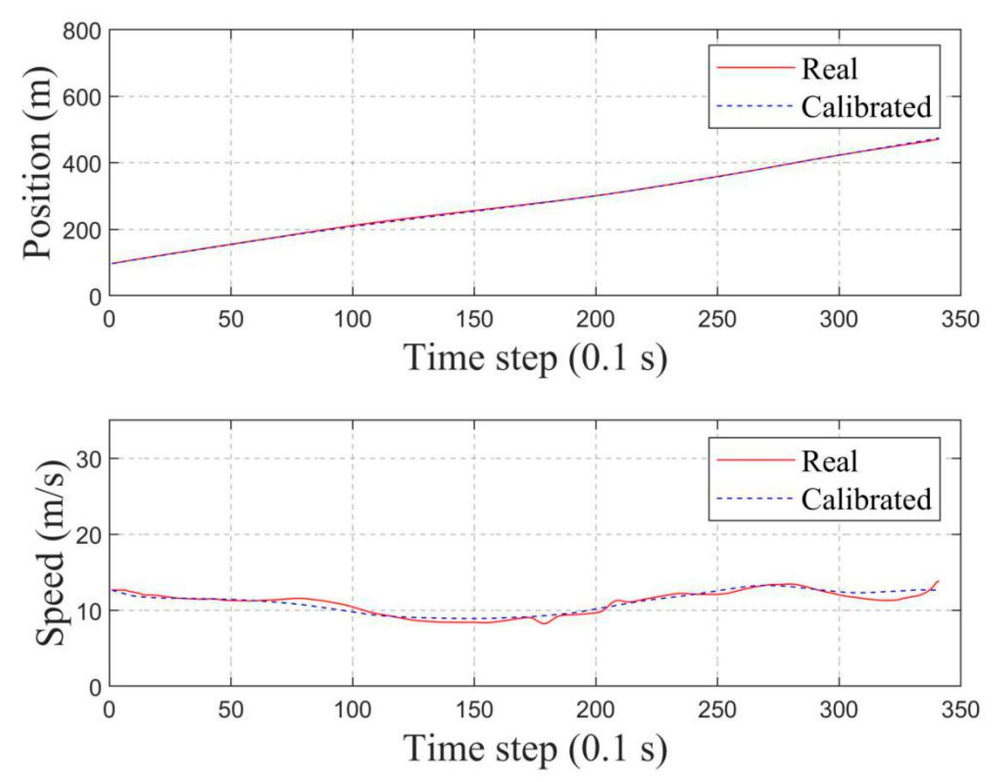
3.1. Results of Parameter Calibration

The trajectory data of each car-following pair were input into the IDM for parameter calibration based on the genetic algorithm. A typical calibration result is presented in Figure 3. The red solid lines represent real positions and speeds while the blue dashed ones denote the calibrated data. It is obvious that the real and calibrated curves overlap almost completely, which indicates good performance of the calibrated IDM for capturing microscopic car-following behaviors.

The statistics of parameter calibrations for the IDM are displayed in

Table 1. Statistics of parameter calibrations for the intelligent driver model (IDM).

Statistics	${\mathbf{s}}_0 \left(\mathbf{m}\right)$	$\mathbf{T}$ (s)	${\mathsf{\alpha }}_{\mathbf{m}} (\mathbf{m}/{\mathbf{s}}^2)$	$\mathsf{\beta }$	${\mathbf{v}}_0 (\mathbf{m}/\mathbf{s})$	Calibrated Objective Value
Mean	0.30	1.19	1.52	3.00	33.34	0.03
Standard deviation	0.92	0.39	0.81	1.95	3.94	0.01
Maximum	5.00	2.00	3.00	5.00	35.00	0.05
Minimum	0.00	0.10	0.50	0.00	20.01	0.01

. Figure 4 depicts distributions of calibrated parameters and calibrated objective values. The calibrated objective values are calculated based on the objective function in Equation (6) and reflect differences between real and calibrated trajectory data and are distributed from 0.01 to 0.05 with a mean of 0.03. The distribution of ${\mathrm{s}}_0$ is mainly concentrated between 0 and 1 m, which is consistent with the congested traffic condition in the NGSIM dataset. The time gap $T$ approximately obeys the normal distribution, with an average gap of 1.19 s. The acceleration and deceleration rates ${\alpha }_m$ and $\beta$, as well as desired maximum speed $v_0$, are also reasonable and in line with the actual situation.

The above calibration results unveil two important facts. First, the applied IDM is able to capture microscopic car-following behaviors extremely well based on parameter values calibrated by the genetic algorithm. The tiny calibrated objective values indicate the good performances of both the IDM and the algorithm. Additionally, distributions of parameter values also imply the apparent individual heterogeneity across human drivers. Most parameters, including $T$, ${\alpha }_m$ and $\beta$, have the obviously distributed values instead of one concentrated value. These results motivate the following safety analysis of individual heterogeneity via simulation experiments.

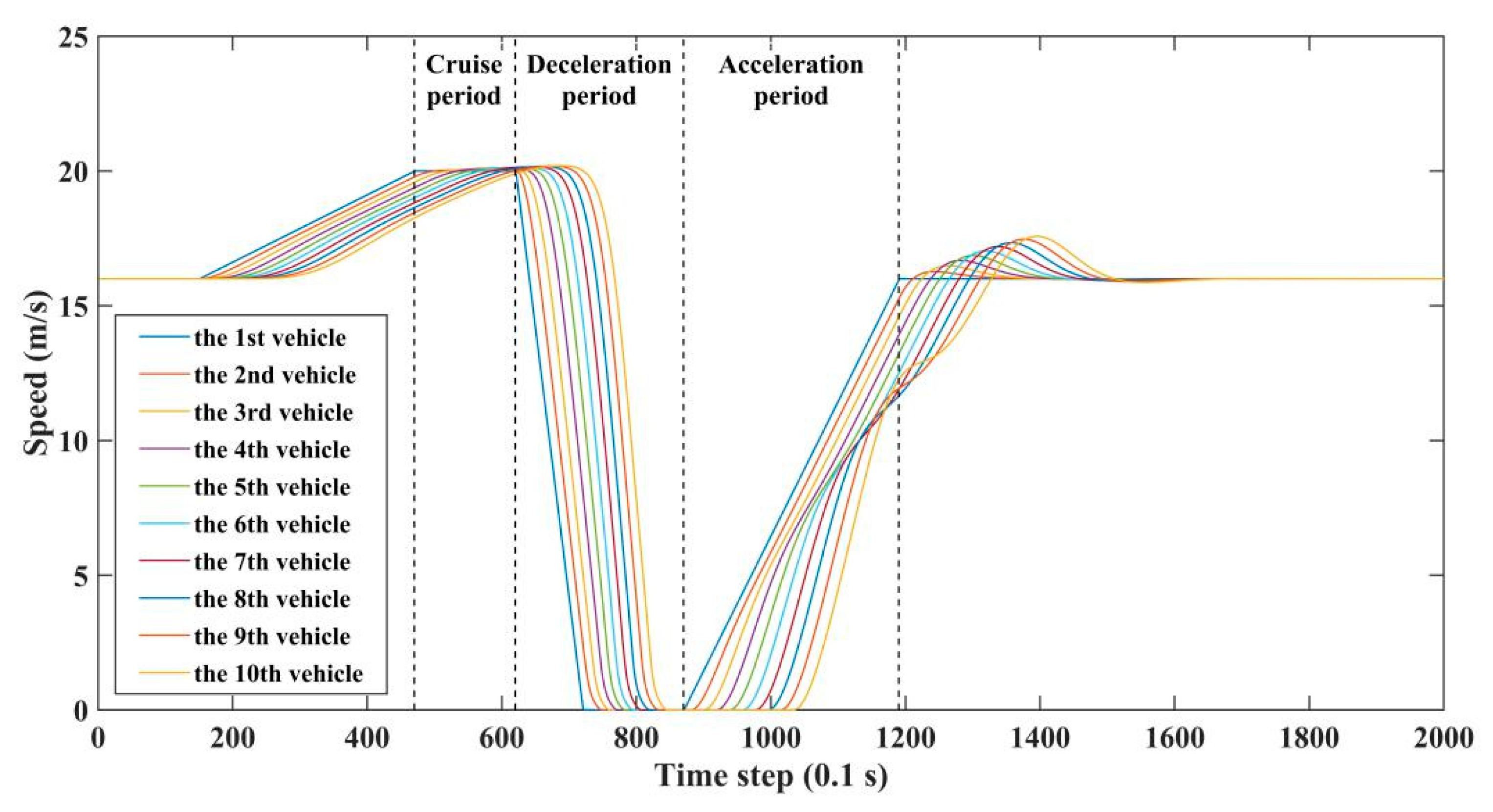
3.2. Traffic Flow of Only Manually Driven Vehicles

This subsection investigated individual heterogeneity in the traffic flow consisting of only manually driven vehicles. The IDM with the fixed parameter values was simulated as the benchmark and the random1 and random2 parameter values were tested for heterogeneity analysis.

In order to simulate the congested traffic condition from the NGSIM dataset, the basic driving cycle of the leading vehicle is set as follows. The leading vehicle is set to drive at a speed of 16 m/s for 15 s; then, it accelerates at a constant acceleration of 1/8 m/s² to reach 20 m/s, and remains this constant speed for 15 s. After that, the leader brakes to standstill at a deceleration rate of 2 m/s² and the stationary state continues for 15 s. Finally, the leading vehicle accelerates at an acceleration of 0.5 m/s² to 16 m/s, and maintains this constant speed to 400 s. All following vehicles make reactions to preceding vehicles’ behaviors based on the IDM. Furthermore, the TET and TIT are calculated based on these TTC values via Equations (8)-(12) for safety evaluations. A typical simulation trajectory is expressed in Figure 5 (excluding the last 200 s of cruise periods for simplicity), which includes cruise, deceleration and acceleration periods.

In the above basic driving cycle, two critical factors were further investigated. One is the simulated vehicle number and the other is the TTC threshold used for determining safe or risky conditions. After preliminary tests, seven different vehicle numbers were finally examined, including 10, 25, 50, 75, 100, 125 and 150 vehicles, as more vehicles do not show a significantly different simulation result. TTC thresholds were set from 1 s to 4 s with an interval of 0.5 s. Results of these simulation experiments are displayed in Figure 6 and Figure 7.

Figure 6 illustrates the heat map results of fixed and random1 parameters. Figure 6a,d shows the TET and TIT results of fixed values, while Figure 6b,e shows to the random1 parameters. Figure 6c,f are TET and TIT results of random1 subtracting those of fixed parameters. It can be observed that all results with randomized parameters are larger than those with fixed values, given the same vehicle number and TTC threshold. For example, the TET and TIT values of random1 parameters are approximately 2.5 times those of fixed parameters with 150 vehicles and the TTC threshold of 2 s. This result indicates that the individual heterogeneity across human drivers remarkably increases rear-end collision risks.

Figure 7 displays the similar comparison results between the fixed and random2 parameters, which demonstrates the negative effects of heterogeneity again. Furthermore, when comparing the results of Figure 6 and Figure 7, it can be observed that the random2 parameters have higher collision risks than those of random1. As aforementioned in Figure 2, parameters in the random2 method are randomly chosen from random1 values, and the former ones possess the much higher degree of individual heterogeneity. Therefore, this result also implies that the higher degree of individual heterogeneity will increase longitudinal collision risks.

Additionally, the growth of simulated vehicle quantities increases the TET and TIT values. The possible explanation for this is that more vehicles will be affected by the leading vehicle with a longer fleet length. Take Figure 6b as an example, the TET values of 25, 50 and 100 vehicles are 189.7, 430.4 and 1071 s, respectively, when TTC threshold is 1 s. It shows that the risks may increase more than two times when the simulation vehicle number doubles. The larger TTC threshold also increases the TET and TIT values, since more conditions will be considered as risky when the threshold value rises. Overall, whatever the simulated vehicle number and TTC threshold are, the negative effects of individual heterogeneity are apparent.

Some may argue that different driving designs of the leading vehicle in simulation experiments will lead to distinct results. After preliminary tests, we figured out that the deceleration rate braking to standstill dominates results of the whole driving process. Therefore, nine different deceleration values were further tested, including 2/5, 1/2, 5/8, 4/5, 1, 5/4, 8/5, 2, and 5/2 m/s², respectively. Note that these rates are not designed to be evenly spaced, since we have to ensure the speeds can be reduced to zero with integer time steps in simulations. The leading vehicle is also set to drive at a speed of 16 m/s for 15 s; then, it accelerates at a constant acceleration of 1/8 m/s² to reach 20 m/s, and remains this constant speed for 15 s. After that, the leader brakes to standstill at various deceleration rates and the stationary state continues for 15 s. Finally, the leading vehicle accelerates at an acceleration of 0.5 m/s² to 16 m/s, and maintains this constant speed to 400 s. A total of 10 vehicles were simulated with the TTC threshold of 2 s.

Figure 8 displays sensitivity analysis results of deceleration rates. For each deceleration value, results of the fixed parameter values are still utilized as the benchmark, and the two random parameters are compared by calculating the changed proportions of TET and TIT. It can be found that changed proportions of both types of random parameters are much larger than zero, no matter which deceleration rate it is. This result demonstrates the negative influence of individual heterogeneity again. It can also be observed that collision risks of random2 parameters are all larger than those of random1, which is consistent with the above finding that the greater degree of heterogeneity causes more remarkable negative impacts on longitudinal safety. In addition, the changed proportion of surrogate safety measures decreases with the increase in the deceleration rate. The reason for this is that with the same speed reduction range in all simulations, a larger deceleration rate will cause a shorter decelerating time.

3.3. Impacts on Mixed Traffic Flow

The aforementioned results imply the significant negative impact of individual heterogeneity in traffic flow consisting of only manually driven vehicles. In this subsection, we further investigated the impacts on mixed traffic flow. The mixed traffic flow consists of manually driven vehicles and ACC vehicles. The driving designs of the leading vehicle was the same as the above settings. A total of 100 vehicles were simulated, with the deceleration rate of 2 m/s² and the TTC threshold of 2 s.

For the mixed traffic flow, the individual heterogeneity includes two aspects, i.e., the heterogeneous behaviors between manually driven vehicles and ACC vehicles, and the heterogeneity within the same type of vehicles. The above simulation experiments in Section 3.2 explored impacts of the heterogeneity within the manually driven vehicles only. In this subsection, the heterogeneity between the two types of vehicles and within ACC vehicles were investigated, which is reflected by the market penetration rate and time gap, respectively. Note that, the heterogeneity within ACC vehicles is not as significant as that of manually driven vehicles, since ACC vehicles are driven based on designed systems. For current commercial ACC vehicles, only the time gap can be selected by drivers and thus the heterogeneity is reflected based on this parameter. The simulated market penetration rate of ACC vehicles ranged from 0% to 100% to examine impacts of the full spectrum. The time gaps of ACC were randomly generated within the interval of $[1.19 s, 1.19\ast \left(1+p\right) s]$, where $p$ was set to be from 0% to 60%.

Figure 9 displays simulation results of the mixed traffic flow. Ten different market penetration rates of ACC vehicles were analyzed, from 0% to 100%. The scenario with a rate of 0% means the traffic flow with only manually driven vehicles. The results show different interaction effects of market penetration rates and time gaps. More specifically, when $p$ is 0% and 10%, the time gaps of all ACC vehicles are about 1.19 s. In this case, the TET and TIT values rise first and then reduce with the increase in market penetration rate, which indicates the negative effects of ACC vehicles in the mixed traffic flow. This result is important since it is contrary to findings of previous studies that ACC vehicles could improve safety. From the perspective of heterogeneity, the ACC vehicle itself is a new source of heterogeneity when mixing with manually driven vehicles and increases the individual heterogeneity.

When $p$ increases to be greater than 20%, the time gaps of most ACC vehicles become larger, and the TET and TIT values decrease monotonously with the increase in market penetration rate. This result is interesting as it indicates that there is a tradeoff between the individual heterogeneity and the time gap of ACC vehicles. On the one hand, the heterogeneity will increase collision risks if different ACC vehicles employ various time gap values. On the other hand, the larger time gap will reduce collision risks with the safer car-following gaps.

The negative safety impacts of individual heterogeneity will definitely compromise the popularization of ACC systems and other similar ICV techniques. Some researchers have found that the presence of novel ICVs in the mixed traffic stream may slow other vehicles down and thus reduce network throughputs [40,41]. Such a phenomenon could last for a long time until the market penetration of ICVs reaches a certain threshold.

Possible countermeasures are inevitable to address the above negative influences. One strategy is to promote ICVs’ applications via various fiscal methods, such as the purchase subsidy and tax reduction. The core idea of fiscal strategy is to increase market penetration rates at the early stage. The other approach is to homogenize traffic flow via transportation safety planning and control. For example, exclusive ICV lanes, ICV roads or even ICV zones have been proposed to separate manually driven vehicles and ICVs [40]. By homogenizing traffic flow, the individual heterogeneity caused by new techniques could be reduced and longitudinal safety may be improved accordingly.

4. Conclusions

This study investigated longitudinal safety influences of individual heterogeneity based on simulation experiments. Two types of vehicle dynamic models were employed to depict driving behaviors of manually driven vehicles and ACC vehicles, respectively. The ACC vehicles can be recognized as low-version autonomous vehicles. Real vehicle trajectories were utilized to calibrate model parameters based on genetic algorithms. Surrogate safety measures were applied to establish the relationship between microscopic behaviors and longitudinal collision risks. Extensive simulation experiments were conducted to evaluate the longitudinal impacts of individual heterogeneity of traffic flow consisting of manually driven vehicles only, as well as mixed traffic flow consisting of both manually driven vehicles and ACC vehicles. The major conclusions we reached consist of the following:

(1)

Individual heterogeneity has negative effects on longitudinal safety—with the higher degree of heterogeneity, longitudinal collision risks are increased.

(2)

Compared to traffic flow consisting of manually driven vehicles only, mixed traffic flow with manually driven vehicles and ACC vehicles may be more dangerous when the market penetration rate of ACC is low, since the ACC system can be recognized as a new source of individual heterogeneity.

We conclude this paper by highlighting the importance of reducing heterogeneity in future mixed traffic consisting of various types of vehicles. Although new ICVs are promising to improve traffic safety, the low market penetration rate and resultant heterogeneous effects are inevitable. There is a lack of systematic methodology to address this issue from the perspective of safety planning, so more research efforts are needed to fill this critical void. Additionally, other relevant factors, such as weather and lighting, may result in heterogeneity, which are also worthy of being further investigated in the future.

References

1. Itasca, I. National Safety Council—Injury Fact; National Safety Council: Itasca, IL, USA, 2015. [Google Scholar]
2. Wu, K.F.; Thor, C.P. Method for the use of naturalistic driving study data to analyze rear-end crash sequences. Transp. Res. Record. 2015, 2518, 27–36. [Google Scholar] [CrossRef]
3. Gao, J.; Davis, G.A. Using naturalistic driving study data to investigate the impact of driver distraction on driver’s brake reaction time in freeway rear-end events in car-following situation. J. Saf. Res. 2017, 63, 195–204. [Google Scholar] [CrossRef]
4. Piccinini, G.B.; Engström, J.; Bärgman, J.; Wang, X. Factors contributing to commercial vehicle rear-end conflicts in China: A study using on-board event data recorders. J. Saf. Res. 2017, 62, 143–153. [Google Scholar] [CrossRef]
5. Wu, Y.; Abdel-Aty, M.; Cai, Q.; Lee, J.; Park, J. Developing an algorithm to assess the rear-end collision risk under fog conditions using real-time data. Transp. Res. Part C-Emerg. Technol. 2018, 87, 11–25. [Google Scholar] [CrossRef]
6. Wu, Y.; Abdel-Aty, M.; Wang, L.; Rahman, M.S. Combined connected vehicles and variable speed limit strategies to reduce rear-end crash risk under fog conditions. J. Intell. Transport. Syst. 2020, 24, 494–513. [Google Scholar] [CrossRef]
7. Christoforou, Z.; Cohen, S.; Karlaftis, M.G. Identifying crash type propensity using real-time traffic data on freeways. J. Saf. Res. 2011, 42, 43–50. [Google Scholar] [CrossRef] [PubMed]
8. Xu, C.; Wang, W.; Liu, P. Identifying crash-prone traffic conditions under different weather on freeways. J. Saf. Res. 2013, 46, 135–144. [Google Scholar] [CrossRef] [PubMed]
9. Xu, C.; Liu, P.; Wang, W.; Li, Z. Identification of freeway crash-prone traffic conditions for traffic flow at different levels of service. Transp. Res. Part A-Policy Pract. 2014, 69, 58–70. [Google Scholar] [CrossRef]
10. Xu, C.; Liu, P.; Yang, B.; Wang, W. Real-time estimation of secondary crash likelihood on freeways using high-resolution loop detector data. Transp. Res. Part C-Emerg. Technol. 2016, 71, 406–418. [Google Scholar] [CrossRef]
11. Pande, A.; Abdel-Aty, M.; Das, A. A classification tree based modeling approach for segment related crashes on multilane highways. J. Saf. Res. 2010, 41, 391–397. [Google Scholar] [CrossRef] [Green Version]
12. Xing, L.; He, J.; Li, Y.; Wu, Y.; Yuan, J.; Gu, X. Comparison of different models for evaluating vehicle collision risks at upstream diverging area of toll plaza. Accid. Anal. Prev. 2020, 135, 105343. [Google Scholar] [CrossRef] [PubMed]
13. Dinu, R.R.; Veeraragavan, A. Random parameter models for accident prediction on two-lane undivided highways in India. J. Saf. Res. 2011, 42, 39–42. [Google Scholar] [CrossRef] [PubMed]
14. Yu, R.; Abdel-Aty, M. Investigating the different characteristics of weekday and weekend crashes. J. Saf. Res. 2013, 46, 91–97. [Google Scholar] [CrossRef] [PubMed]
15. Xing, L.; He, J.; Abdel-Aty, M.; Cai, Q.; Li, Y.; Zheng, O. Examining traffic conflicts of up stream toll plaza area using vehicles’ trajectory data. Accid. Anal. Prev. 2019, 125, 174–187. [Google Scholar] [CrossRef]
16. Xing, L.; He, J.; Abdel-Aty, M.; Wu, Y.; Yuan, J. Time-varying Analysis of Traffic Conflicts in Toll Plaza’s Upstream Diverging Area. Accid. Anal. Prev. 2020, 141, 105539. [Google Scholar] [CrossRef]
17. Behnood, A.; Mannering, F. The effect of passengers on driver-injury severities in single-vehicle crashes: A random parameters heterogeneity-in-means approach. Anal. Methods Accid. Res. 2017, 14, 41–53. [Google Scholar] [CrossRef]
18. Li, Y.; Xu, C.; Xing, L.; Wang, W. Integrated cooperative adaptive cruise and variable speed limit controls for reducing rear-end collision risks near freeway bottlenecks based on micro-simulations. IEEE Trans. Intell. Transp. Syst. 2017, 18, 3157–3167. [Google Scholar] [CrossRef]
19. Li, Y.; Wang, H.; Wang, W.; Xing, L.; Liu, S.; Wei, X. Evaluation of the impacts of cooperative adaptive cruise control on reducing rear-end collision risks on freeways. Accid. Anal. Prev. 2017, 98, 87–95. [Google Scholar] [CrossRef]
20. Li, Y.; Xing, L.; Wang, W.; Wang, H.; Dong, C.; Liu, S. Evaluating impacts of different longitudinal driver assistance systems on reducing multi-vehicle rear-end crashes during small-scale inclement weather. Accid. Anal. Prev. 2017, 107, 63–76. [Google Scholar] [CrossRef]
21. Li, Y.; Li, Z.; Wang, H.; Wang, W.; Xing, L. Evaluating the safety impact of adaptive cruise control in traffic oscillations on freeways. Accid. Anal. Prev. 2017, 104, 137–145. [Google Scholar] [CrossRef]
22. Li, Y.; Tu, Y.; Fan, Q.; Dong, C.; Wang, W. Influence of cyber-attacks on longitudinal safety of connected and automated vehicles. Accid. Anal. Prev. 2018, 121, 148–156. [Google Scholar] [CrossRef] [PubMed]
23. Xu, C.; Ding, Z.; Wang, C.; Li, Z. Statistical analysis of the patterns and characteristics of connected and autonomous vehicle involved crashes. J. Saf. Res. 2019, 71, 41–47. [Google Scholar] [CrossRef] [PubMed]
24. Li, Y.; Chen, Z.; Yin, Y.; Peeta, S. Deployment of roadside units to overcome connectivity gap in transportation networks with mixed traffic. Transp. Res. Part C-Emerg. Technol. 2020, 111, 496–512. [Google Scholar] [CrossRef]
25. Treiber, M.; Hennecke, A.; Helbing, D. Congested traffic states in empirical observations and microscopic simulations. Phys. Rev. E 2000, 62, 1805. [Google Scholar] [CrossRef] [Green Version]
26. Rahman, M.S.; Abdel-Aty, M. Longitudinal safety evaluation of connected vehicles’ platooning on expressways. Accid. Anal. Prev. 2018, 117, 381–391. [Google Scholar] [CrossRef]
27. Zheng, Y.; Zhang, G.; Li, Y.; Li, Z. Optimal jam-absorption driving strategy for mitigating rear-end collision risks with oscillations on freeway straight segments. Accid. Anal. Prev. 2020, 135, 105367. [Google Scholar] [CrossRef]
28. Milanés, V.; Shladover, S.E.; Spring, J.; Nowakowski, C.; Kawazoe, H.; Nakamura, M. Cooperative adaptive cruise control in real traffic situations. IEEE Trans. Intell. Transp. Syst. 2013, 15, 296–305. [Google Scholar] [CrossRef] [Green Version]
29. Milanés, V.; Shladover, S.E. Modeling cooperative and autonomous adaptive cruise control dynamic responses using experimental data. Transp. Res. Part C-Emerg. Technol. 2014, 48, 285–300. [Google Scholar] [CrossRef] [Green Version]
30. Xiao, L.; Wang, M.; Schakel, W.; Van Arem, B. Unravelling effects of cooperative adaptive cruise control deactivation on traffic flow characteristics at merging bottlenecks. Transp. Res. Part C-Emerg. Technol. 2018, 96, 380–397. [Google Scholar] [CrossRef]
31. FHWA. Next Generation Simulation (NGSIM). 2006. Available online: https://ops.fhwa.dot.gov/trafficanalysistools/ngsim.htm (accessed on 1 December 2006).
32. Kesting, A.; Treiber, M.; Schönhof, M.; Kranke, F.; Helbing, D. Jam-avoiding adaptive cruise control (ACC) and its impact on traffic dynamics. In Traffic and Granular Flow’05; Springer: Berlin/Heidelberg, Germany, 2007; pp. 633–643. [Google Scholar]
33. Kesting, A.; Treiber, M.; Schönhof, M.; Helbing, D. Adaptive cruise control design for active congestion avoidance. Transp. Res. Part C-Emerg. Technol. 2008, 16, 668–683. [Google Scholar] [CrossRef]
34. Kusano, K.D.; Chen, R.; Montgomery, J.; Gabler, H.C. Population distributions of time to collision at brake application during car following from naturalistic driving data. J. Saf. Res. 2015, 54, 95.e29–104. [Google Scholar]
35. Lubbe, N. Brake reactions of distracted drivers to pedestrian Forward Collision Warning systems. J. Saf. Res. 2017, 61, 23–32. [Google Scholar]
36. Tu, Y.; Wang, W.; Li, Y.; Xu, C.; Xu, T.; Li, X. Longitudinal safety impacts of cooperative adaptive cruise control vehicle’s degradation. J. Saf. Res. 2019, 69, 177–192. [Google Scholar]
37. Li, Y.; Wu, D.; Lee, J.; Yang, M.; Shi, Y. Analysis of the transition condition of rear-end collisions using time-to-collision index and vehicle trajectory data. Accid. Anal. Prev. 2020, 144, 105676. [Google Scholar] [PubMed]
38. Minderhoud, M.M.; Bovy, P.H. Extended time-to-collision measures for road traffic safety assessment. Accid. Anal. Prev. 2001, 33, 89–97. [Google Scholar]
39. Meng, Q.; Qu, X. Estimation of rear-end vehicle crash frequencies in urban road tunnels. Accid. Anal. Prev. 2012, 48, 254–263. [Google Scholar]
40. Chen, Z.; He, F.; Yin, Y.; Du, Y. Optimal design of autonomous vehicle zones in transportation networks. Transp. Res. Part B-Methodol. 2017, 99, 44–61. [Google Scholar]
41. Calvert, S.C.; Schakel, W.J.; Van Lint, J.W.C. Will automated vehicles negatively impact traffic flow? J. Adv. Transp. 2017, 2017, 3082781. [Google Scholar]
Figure 1. Illustration of the research framework.
Sustainability 12 08941 g001
Figure 2. The process of parameter calibration and randomization designs.
Sustainability 12 08941 g002
Figure 3. Typical calibration results.
Sustainability 12 08941 g003
Figure 4. Distributions of calibrated parameter values.
Sustainability 12 08941 g004
Figure 5. Illustration of simulated trajectories (ten vehicles).
Sustainability 12 08941 g005
Figure 6. Simulation results between fixed and random1 parameters, (a) TET for fixed parameters, (b) TET for random1 parameters, (c) TET for difference between the random1 and fixed parameters, (d) TIT for fixed parameters, (e) TIT for random1 parameters, (f) TIT for difference between the random1 and fixed parameters.
Sustainability 12 08941 g006
Figure 7. Simulation results between fixed and random2 parameters, (a) TET for fixed parameters, (b) TET for random2 parameters, (c) TET for difference between the random2 and fixed parameters, (d) TIT for fixed parameters, (e) TIT for random2 parameters, (f) TIT for difference between the random2 and fixed parameters.
Sustainability 12 08941 g007
Figure 8. Sensitivity analysis of deceleration rates: (a) time integrated time-to collision (TIT); (b) time exposed time-to-collision (TET).
Sustainability 12 08941 g008
Figure 9. Results of mixed traffic flow with adaptive cruise control (ACC) vehicles: (a) TIT; (b) TET.
Sustainability 12 08941 g009