Home-Based Locational Accessibility to Essential Urban Services: The Case of Wake County, North Carolina, USA


Abstract
:1. Introduction
2. Literature Review
2.1. Accessibility Measures
2.2. Accessibility Applications
2.3. Locational Accessibility as Used in This Research
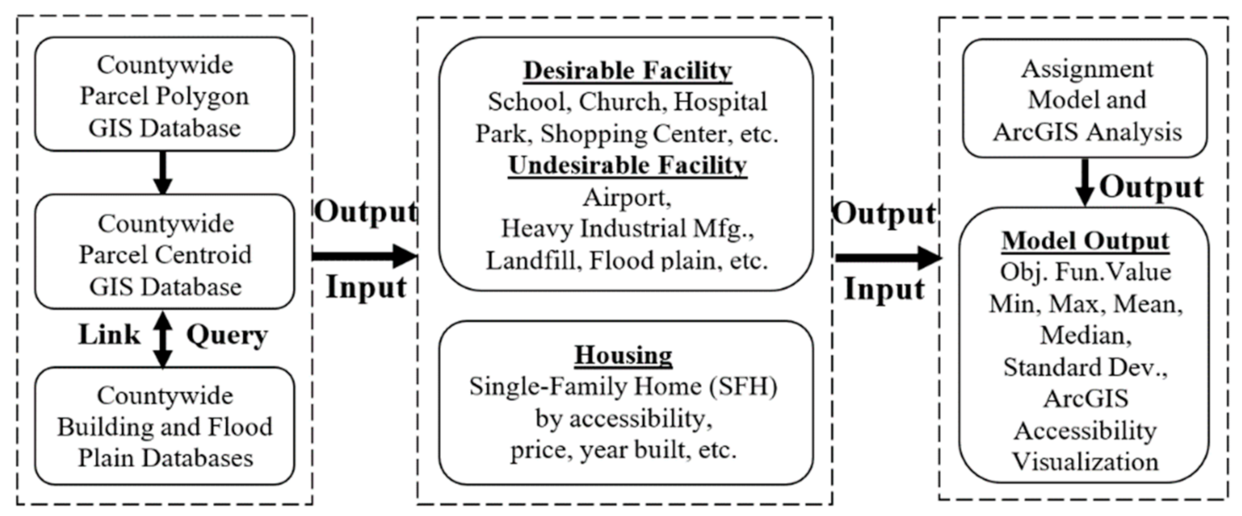
3. Methodology
3.1. Model Assumptions
3.2. Model Formulation
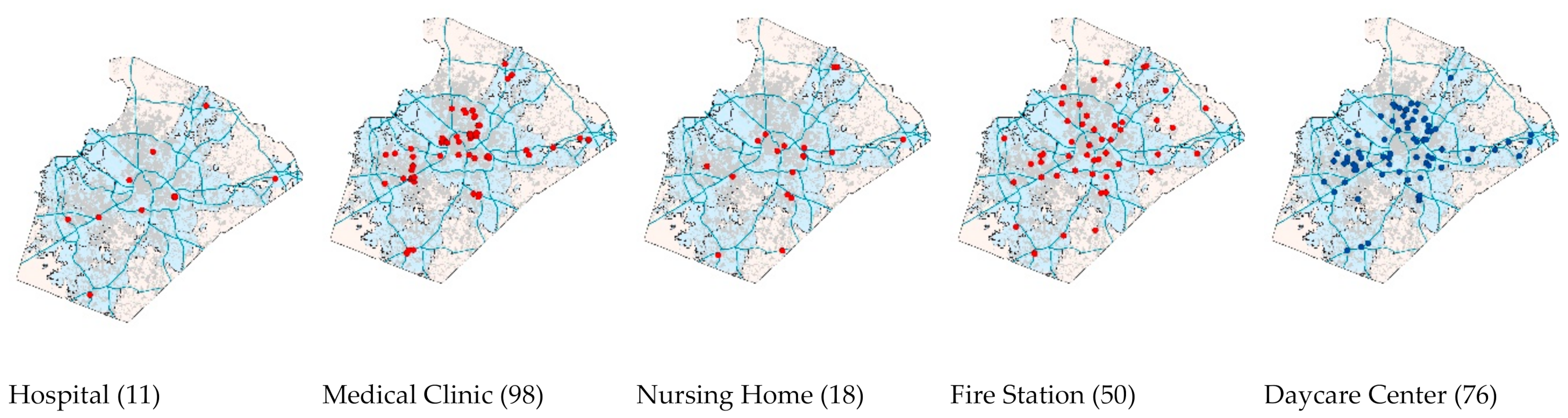
3.3. Study Site and Database
3.4. Modeling Procedure
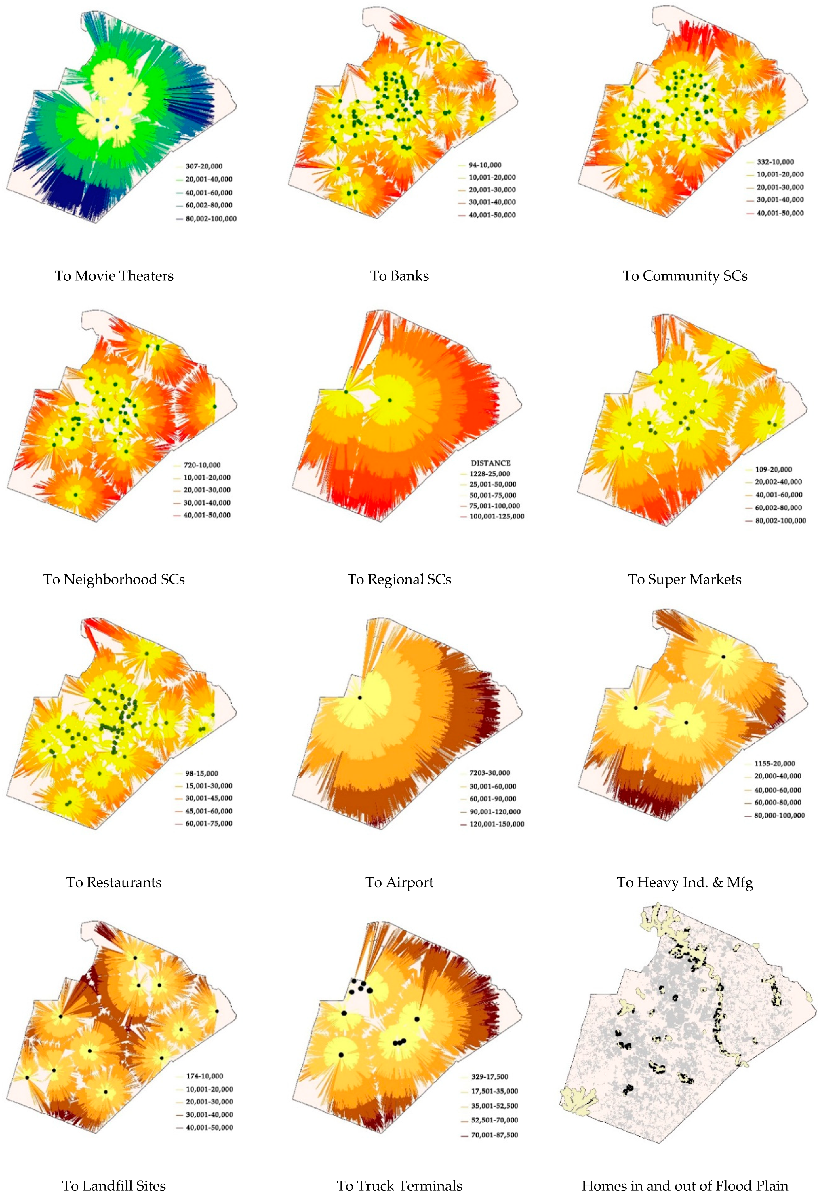
4. Results and Discussions
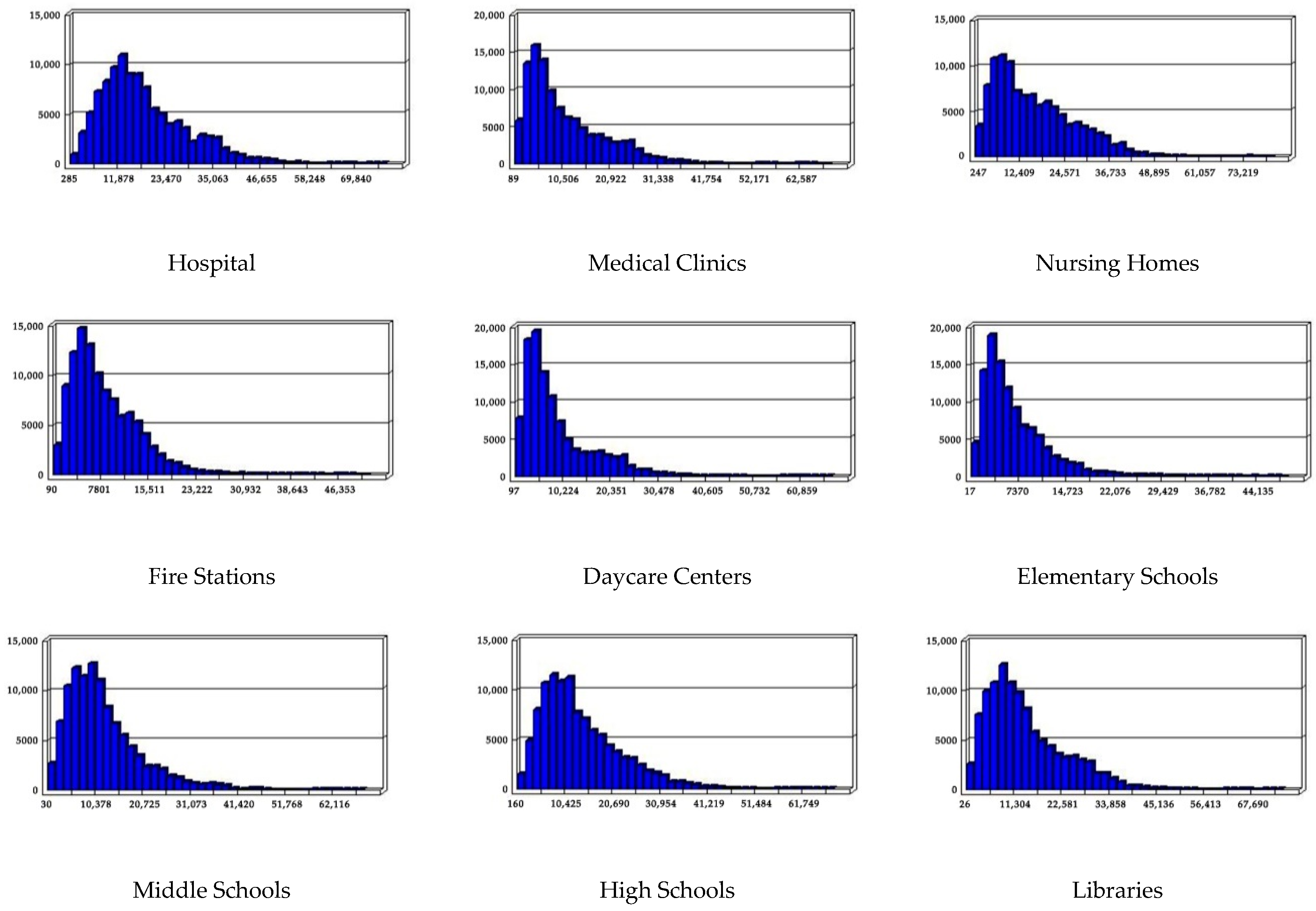
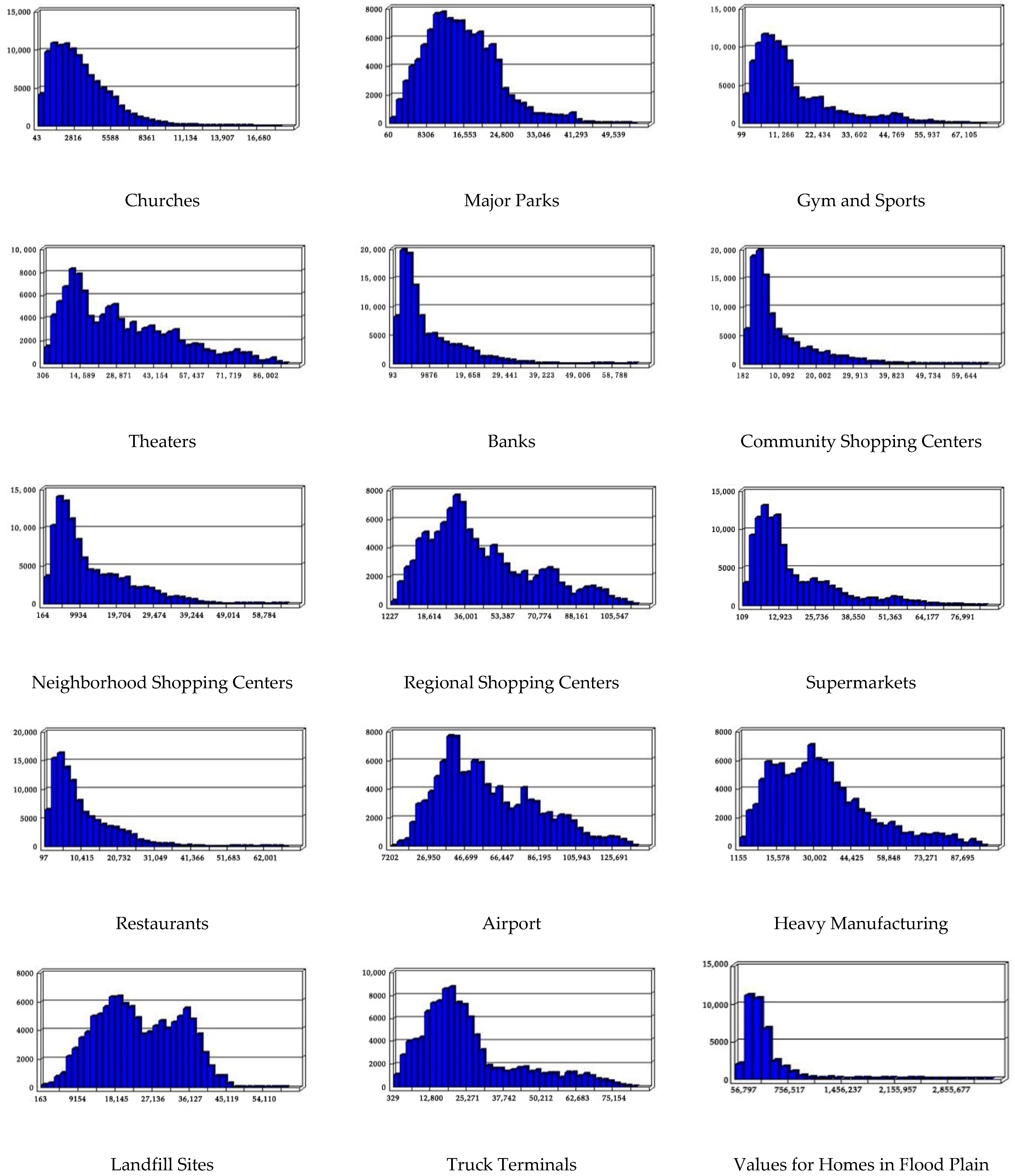
4.1. Key Statistics for Accessibility
4.2. Accessibility Disparity by Home Value and Year Built?
4.3. Home-Based Accessibility Good to Explain Home Value?
5. Conclusions and Remarks
Author Contributions
Funding
Acknowledgments
Conflicts of Interest
References
- Haase, D.; Güneralp, B.; Dahiya, B.; Bai, X.; Elmqvist, T. Global urbanization. Urban Planet Knowl. Towards Sustain. Cities 2018, 19, 326–339. [Google Scholar]
- Glaeser, E.L. Triumph of the city: How our greatest invention makes us richer, smarter, greener, healthier, and happier (an excerpt). J. Econ. Sociol. 2013, 14, 75–94. [Google Scholar] [CrossRef]
- Cervero, R.; Rood, T.; Appleyard, B. Tracking accessibility: Employment and housing opportunities in the San Francisco Bay Area. Environ. Plan. A 1999, 31, 1259–1278. [Google Scholar] [CrossRef]
- Geurs, K.T.; Krizek, K.J.; Reggiani, A. Accessibility Analysis and Transport Planning: Challenges for Europe and North America; Edward Elgar Publishing: Cheltenham, UK, 2012. [Google Scholar]
- Harvard. The State of the Nation’s Housing. Available online: https://www.jchs.harvard.edu/sites/default/files/Harvard_JCHS_State_of_the_Nations_Housing_2018.pdf (accessed on 20 May 2020).
- Geurs, K.T.; Van Wee, B. Accessibility evaluation of land-use and transport strategies: Review and research directions. J. Transp. Geogr. 2004, 12, 127–140. [Google Scholar] [CrossRef]
- Wilson, S.; Hutson, M.; Mujahid, M. How planning and zoning contribute to inequitable development, neighborhood health, and environmental injustice. Environ. Justice 2008, 1, 211–216. [Google Scholar] [CrossRef] [Green Version]
- Curl, A.; Nelson, J.D.; Anable, J. Does accessibility planning address what matters? A review of current practice and practitioner perspectives. Res. Transp. Bus. Manag. 2011, 2, 3–11. [Google Scholar] [CrossRef] [Green Version]
- Johnson, D.; Ercolani, M.; Mackie, P. Econometric analysis of the link between public transport accessibility and employment. Transp. Policy 2017, 60, 1–9. [Google Scholar] [CrossRef]
- McKeown, P.; Workman, B. A study in using linear programming to assign students to schools. Interfaces 1976, 6, 96–101. [Google Scholar] [CrossRef]
- Mei, D.; Xiu, C.; Feng, X.; Wei, Y. Study of the School–Residence Spatial Relationship and the Characteristics of Travel-to-School Distance in Shenyang. Sustainability 2019, 11, 4432. [Google Scholar] [CrossRef] [Green Version]
- Swersey, A.J.; Ballard, W. Scheduling school buses. Manag. Sci. 1984, 30, 844–853. [Google Scholar] [CrossRef]
- Bowen, W.M.; Salling, M.J.; Haynes, K.E.; Cyran, E.J. Toward environmental justice: Spatial equity in Ohio and Cleveland. Ann. Assoc. Am. Geogr. 1995, 85, 641–663. [Google Scholar] [CrossRef]
- Martens, K. Justice in transport as justice in accessibility: Applying Walzer’s ‘Spheres of Justice’to the transport sector. Transportation 2012, 39, 1035–1053. [Google Scholar] [CrossRef] [Green Version]
- Omer, I. Evaluating accessibility using house-level data: A spatial equity perspective. Comput. Environ. Urban Syst. 2006, 30, 254–274. [Google Scholar] [CrossRef]
- Hansen, W.G. How accessibility shapes land use. J. Am. Inst. Plan. 1959, 25, 73–76. [Google Scholar] [CrossRef]
- Dong, X.; Ben-Akiva, M.E.; Bowman, J.L.; Walker, J.L. Moving from trip-based to activity-based measures of accessibility. Transp. Res. Part A Policy Pract. 2006, 40, 163–180. [Google Scholar] [CrossRef]
- Handy, S.L.; Niemeier, D.A. Measuring accessibility: An exploration of issues and alternatives. Environ. Plan. A 1997, 29, 1175–1194. [Google Scholar] [CrossRef]
- Koenig, J.G. Indicators of urban accessibility: Theory and application. Transportation 1980, 9, 145–172. [Google Scholar] [CrossRef]
- Van Wee, B. Accessible accessibility research challenges. J. Transp. Geogr. 2016, 51, 9–16. [Google Scholar] [CrossRef] [Green Version]
- Wachs, M.; Kumagai, T.G. Physical accessibility as a social indicator. Socio-Econ. Plan. Sci. 1973, 7, 437–456. [Google Scholar] [CrossRef]
- Bhat, C.; Handy, S.; Kockelman, K.; Mahmassani, H.; Chen, Q.; Weston, L. Development of an Urban Accessibility Index: Literature Review; University of Texas at Austin. Center for Transportation Research: Austin, TX, USA, 2000. [Google Scholar]
- Farrington, J.H. The new narrative of accessibility: Its potential contribution to discourses in (transport) geography. J. Transp. Geogr. 2007, 15, 319–330. [Google Scholar] [CrossRef]
- Neuburger, H. User benefit in the evaluation of transport and land use plans. J. Transp. Econ. Policy 1971, 5, 52–75. [Google Scholar]
- Vickerman, R.W. Accessibility, attraction, and potential: A review of some concepts and their use in determining mobility. Environ. Plan. A 1974, 6, 675–691. [Google Scholar] [CrossRef] [Green Version]
- Wubneh, M.; Shen, G. The impact of manufactured housing on adjacent residential property values: A GIS approach based on three North Carolina counties. Rev. Urban Reg. Dev. Stud. 2004, 16, 56–73. [Google Scholar] [CrossRef]
- Ben-Akiva, M.E.; Lerman, S.R.; Lerman, S.R. Discrete Choice Analysis: Theory and Application to Travel Demand; MIT Press: Cambridge, MA, USA, 1985. [Google Scholar]
- Chorus, C.G.; De Jong, G.C. Modeling experienced accessibility for utility-maximizers and regret-minimizers. J. Transp. Geogr. 2011, 19, 1155–1162. [Google Scholar] [CrossRef]
- Miller, H.J. Place-based versus people-based accessibility. In LEVINSON, D AND KRIZEK, KJ Access to Destinations; Elsevier: Oxford, UK, 2005; pp. 63–89. [Google Scholar]
- Wu, Y.H.; Miller, H.J. Computational tools for measuring space-time accessibility within dynamic flow transportation networks. J. Transp. Stat. 2001, 4, 1–14. [Google Scholar]
- Li, Q.; Zhang, T.; Wang, H.; Zeng, Z. Dynamic accessibility mapping using floating car data: A network-constrained density estimation approach. J. Transp. Geogr. 2011, 19, 379–393. [Google Scholar] [CrossRef]
- Santos, F.; Almeida, A.; Martins, C.; Gonçalves, R.; Martins, J. Using POI functionality and accessibility levels for delivering personalized tourism recommendations. Comput. Environ. Urban Syst. 2019, 77, 101173. [Google Scholar] [CrossRef]
- Shen, G. Location of manufactured housing and its accessibility to community services: A GIS-assisted spatial analysis. Socio-Econ. Plan. Sci. 2005, 39, 25–41. [Google Scholar] [CrossRef]
- Srour, I.M.; Kockelman, K.M.; Dunn, T.P. Accessibility indices: Connection to residential land prices and location choices. Transp. Res. Rec. 2002, 1805, 25–34. [Google Scholar] [CrossRef] [Green Version]
- Giuliano, G.; Gordon, P.; Pan, Q.; Park, J. Accessibility and residential land values: Some tests with new measures. Urban Stud. 2010, 47, 3103–3130. [Google Scholar] [CrossRef] [Green Version]
- Horner, M.W. Spatial dimensions of urban commuting: A review of major issues and their implications for future geographic research. Prof. Geogr. 2004, 56, 160–173. [Google Scholar]
- Talen, E.; Anselin, L. Assessing spatial equity: An evaluation of measures of accessibility to public playgrounds. Environ. Plan. A 1998, 30, 595–613. [Google Scholar] [CrossRef] [Green Version]
- Coutts, C. Greenway accessibility and physical-activity behavior. Environ. Plan. B Plan. Des. 2008, 35, 552–563. [Google Scholar] [CrossRef] [Green Version]
- Boone, C.G.; Buckley, G.L.; Grove, J.M.; Sister, C. Parks and people: An environmental justice inquiry in Baltimore, Maryland. Ann. Assoc. Am. Geogr. 2009, 99, 767–787. [Google Scholar] [CrossRef]
- Rigolon, A. A complex landscape of inequity in access to urban parks: A literature review. Landsc. Urban Plan. 2016, 153, 160–169. [Google Scholar] [CrossRef]
- Iraegui, E.; Augusto, G.; Cabral, P. Assessing Equity in the Accessibility to Urban Green Spaces According to Different Functional Levels. Isprs Int. J. Geo-Inf. 2020, 9, 308. [Google Scholar] [CrossRef]
- Khan, A.A. An integrated approach to measuring potential spatial access to health care services. Socio-Econ. Plan. Sci. 1992, 26, 275–287. [Google Scholar] [CrossRef]
- Luo, W.; Wang, F. Measures of spatial accessibility to health care in a GIS environment: Synthesis and a case study in the Chicago region. Environ. Plan. B Plan. Des. 2003, 30, 865–884. [Google Scholar] [CrossRef] [Green Version]
- Bissonnette, L.; Wilson, K.; Bell, S.; Shah, T.I. Neighbourhoods and potential access to health care: The role of spatial and aspatial factors. Health Place 2012, 18, 841–853. [Google Scholar] [CrossRef] [Green Version]
- Bell, S.; Wilson, K.; Bissonnette, L.; Shah, T. Access to primary health care: Does neighborhood of residence matter? Ann. Assoc. Am. Geogr. 2013, 103, 85–105. [Google Scholar] [CrossRef]
- Paul, A. Land-use-accessibility model: A theoretical approach to capturing land-use influence on vehicular flows through configurational measures of spatial networks. Int. J. Urban Sci. 2012, 16, 225–241. [Google Scholar] [CrossRef]
- Vandebona, U.; Tsukaguchi, H. Impact of urbanization on user expectations related to public transport accessibility. Int. J. Urban Sci. 2013, 17, 199–211. [Google Scholar] [CrossRef]
- Jang, S.; An, Y.; Yi, C.; Lee, S. Assessing the spatial equity of Seoul’s public transportation using the Gini coefficient based on its accessibility. Int. J. Urban Sci. 2017, 21, 91–107. [Google Scholar] [CrossRef]
- Mladenka, K.R. The distribution of an urban public service: The changing role of race and politics. Urban Aff. Q. 1989, 24, 556–583. [Google Scholar] [CrossRef]
- Hewko, J.; Smoyer-Tomic, K.E.; Hodgson, M.J. Measuring neighbourhood spatial accessibility to urban amenities: Does aggregation error matter? Environ. Plan. A 2002, 34, 1185–1206. [Google Scholar] [CrossRef]
- Gonzalez-Feliu, J.; Salanova Grau, J.M.; Beziat, A. A location-based accessibility analysis to estimate the suitability of urban consolidation facilities. Int. J. Urban Sci. 2014, 18, 166–185. [Google Scholar] [CrossRef]
- Shen, G. Measuring accessibility of housing to public–community facilities using Geographical Information Systems. Rev. Urban Reg. Dev. Stud. 2002, 14, 235–255. [Google Scholar] [CrossRef]
- Taaffe, E.J.; Gauthier, H.; O’Kelly, M.E. Geography of Transportation; Prentice Hall: Englewood, FL, USA, 1996. [Google Scholar]
- Shogan, A.W. Management Science; Prentice Hall: Englewood, FL, USA, 1998. [Google Scholar]
- Wu, W.; Gan, A.; Cevallos, F.; Shen, L.D. Selecting bus stops for accessibility improvements for riders with physical disabilities. J. Public Transp. 2011, 14, 133–149. [Google Scholar] [CrossRef] [Green Version]
- Feng, S.; Chen, L.; Sun, R.; Feng, Z.; Li, J.; Khan, M.S.; Jing, Y. The Distribution and Accessibility of Urban Parks in Beijing, China: Implications of Social Equity. Int. J. Environ. Res. Public Health 2019, 16, 4894. [Google Scholar] [CrossRef] [PubMed] [Green Version]
- Alonso, W. Location and Land Use: Toward A General Theory of Land Rent; Harvard University Press: Cambridge, MA, USA, 1964. [Google Scholar]
- Harris, C.D.; Ullman, E.L. The nature of cities. Annu. Am. Acad. Political Soc. Sci. 1945, 242, 7–17. [Google Scholar] [CrossRef]


| 1. For Environmental, Health, and Rescue Services | ||||||
| Facility Type | Number | Min | Max | Mean | Median | Std. Dev. |
| Hospital | 11 | 286.53 | 76,689.13 | 17,955.57 | 15,803.93 | 10,287.93 |
| Medical Clinic | 98 | 89.92 | 68,740.91 | 10,718.26 | 7940.29 | 8323.12 |
| Nursing Home | 18 | 247.53 | 80,411.53 | 15,946.60 | 13,549.54 | 10,797.36 |
| Fire Station | 50 | 90.64 | 50,908.50 | 8109.94 | 6820.35 | 5281.50 |
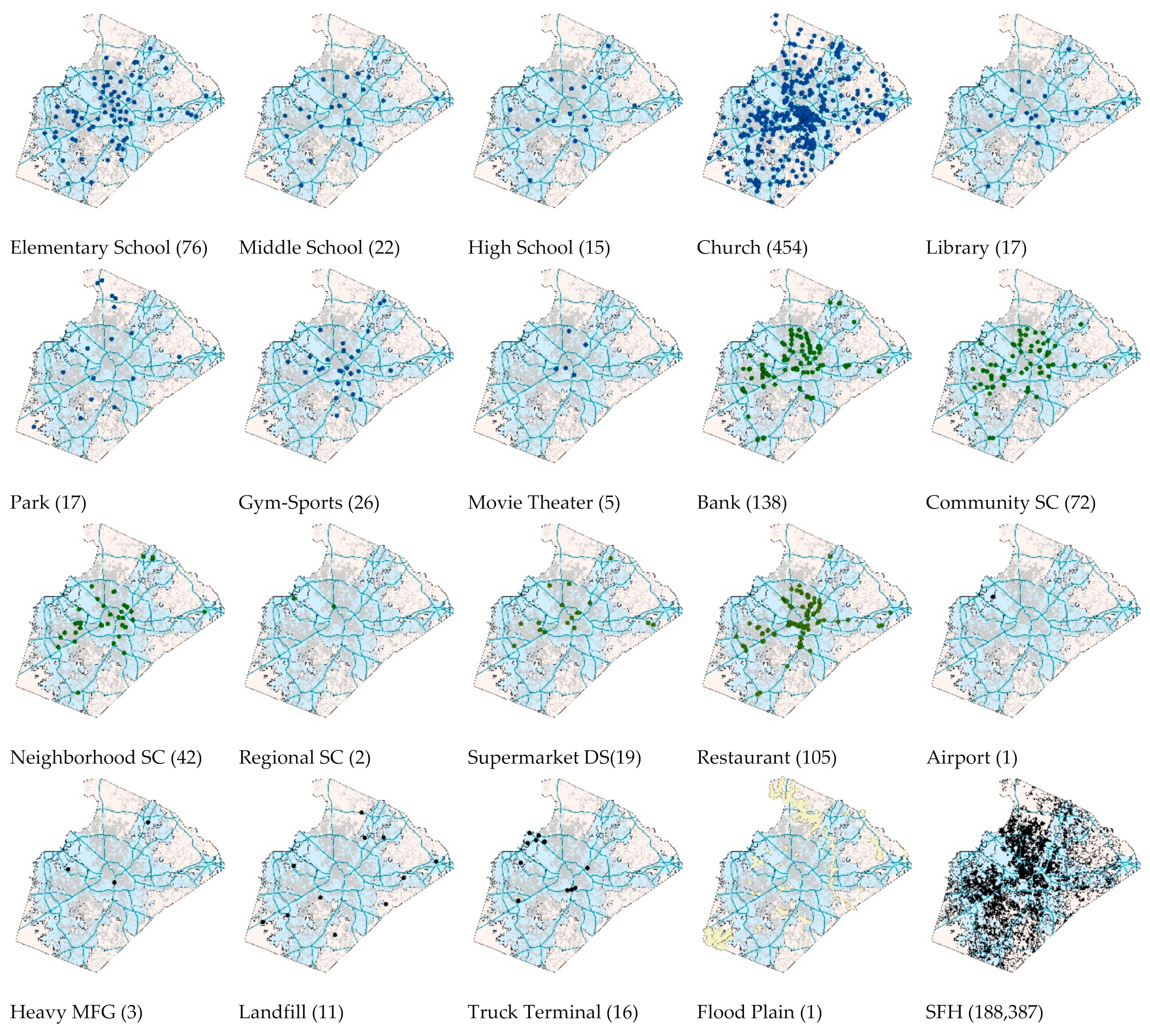
| 2. For Cultural, Recreational, and Educational Services | ||||||
| Daycare Center | 76 | 97.25 | 6684.57 | 8820.28 | 6212.95 | 7556.96 |
| Elementary School | 76 | 17.82 | 48,479.62 | 6589.45 | 5081.21 | 5184.24 |
| Middle School | 22 | 30.76 | 68,228.97 | 11,877.17 | 10,119.14 | 7961.07 |
| High School | 15 | 160.48 | 67,813.10 | 13,548.65 | 11,441.80 | 8425.99 |
| Church | 454 | 43.17 | 18,318.39 | 3170.53 | 2744.24 | 2121.99 |
| Library | 17 | 26.75 | 74,353.04 | 13,627.16 | 11,392.39 | 9050.61 |
| Park | 17 | 60.39 | 54,411.34 | 15,957.97 | 15,075.14 | 8123.12 |
| Gym and Sports | 26 | 98.98 | 73,702.58 | 14,580.26 | 10,986.14 | 11,930.28 |
| Theater | 5 | 306.59 | 94,440.04 | 29,806.50 | 25,269.30 | 20,802.51 |
| 3. For Auto, Food, Shopping, and Other Business Services | ||||||
| Bank | 138 | 93.75 | 64,567.70 | 8778.47 | 5776.70 | 7785.93 |
| Community Shopping Center | 72 | 182.10 | 65,499.29 | 9471.35 | 6069.10 | 8632.97 |
| Neighborhood Shopping Center | 42 | 164.91 | 64,556.54 | 12,070.07 | 8649.34 | 9399.92 |
| Regional Shopping Center | 2 | 1227.62 | 115,819.10 | 42,632.23 | 36,380.51 | 24,334.71 |
| Supermarket | 19 | 109.45 | 84,561.00 | 17,126.21 | 11,965.78 | 14,665.02 |
| Restaurant | 105 | 97.84 | 68,096.04 | 9876.25 | 7351.71 | 7842.14 |
| 4. For Manufacturing, Waste Management, and Transportation Services | ||||||
| Airport | 1 | 7202.66 | 137,358.28 | 58,645.84 | 53,252.05 | 25,959.90 |
| Heavy Manufacturing, | 3 | 1155.38 | 96,215.82 | 32,351.88 | 29,479.66 | 21,048.51 |
| Landfill | 11 | 163.02 | 59,422.03 | 23,741.26 | 22,734.43 | 9983.33 |
| Truck Terminal | 16 | 329.31 | 82,522.07 | 25,361.52 | 20,354.66 | 16,627.83 |
| 1. For Environmental, Health, and Rescue Services | ||||||||
| Facility Type | 50 k–125 k | 125 k–200 k | 200 k–275 k | 275 k–350 k | 350 k–425 k | 425 k–500 k | 500 k–700 k | >700 k |
| Hospitals | 18,360.48 | 19,793.90 | 18,931.54 | 17,356.94 | 16,220.01 | 16,542.93 | 15,554.63 | 14,845.34 |
| Medical Clinic | 12,444.23 | 11,996.88 | 12,024.41 | 10,000.47 | 9313.55 | 9823.56 | 8149.82 | 6327.46 |
| Nursing Home | 14,534.09 | 13,347.44 | 15,912.32 | 17,355.55 | 17,165.87 | 17,791.88 | 15,387.10 | 11,310.30 |
| Fire Station | 7995.51 | 7762.26 | 8261.98 | 8209.36 | 7978.27 | 7971.17 | 7827.22 | 6831.82 |
| 2. For Cultural, Recreational, and Educational Services | ||||||||
| Daycare Center | 9809.03 | 8830.10 | 9119.62 | 8030.86 | 7809.81 | 8970.98 | 8009.06 | 7828.34 |
| Elementary School | 7564.93 | 6939.77 | 6972.22 | 6372.15 | 5844.14 | 5895.90 | 5640.94 | 4901.31 |
| Middle School | 14,594.33 | 13,690.69 | 12,817.30 | 10,431.53 | 10,521.30 | 11,163.99 | 9956.03 | 8177.71 |
| High School | 14,299.25 | 14,323.72 | 13,996.90 | 12,216.02 | 12,783.88 | 13,734.42 | 12,937.14 | 11,546.26 |
| Church | 2563.47 | 2962.92 | 3200.28 | 3130.25 | 3137.13 | 3422.89 | 3239.55 | 3326.87 |
| Library | 12,809.65 | 11,963.96 | 13,613.41 | 13,528.04 | 14,024.46 | 15,020.65 | 13,477.21 | 11,963.87 |
| Park | 18,704.84 | 18,419.21 | 16,084.12 | 13,722.33 | 13,647.49 | 14,543.07 | 15,400.00 | 17,865.30 |
| Gym-Sports | 17,949.50 | 14,852/12 | 15,166.82 | 13,355.45 | 13,648.69 | 14,261.13 | 12,578.82 | 10,692.15 |
| Theater | 40,832.12 | 34,950.23 | 32,363.21 | 28,115.43 | 25,270.92 | 24,043.48 | 21,200.65 | 18,554.67 |
| 3. For Auto, Food, Shopping, and Other Business Services | ||||||||
| Bank | 10,019.63 | 10,023.41 | 9552.10 | 8217.68 | 7490.47 | 7820.22 | 6703.38 | 6033.47 |
| Community Shopping Center | 12,005.66 | 10,923.71 | 10,114.54 | 8735.50 | 7933.47 | 8215.89 | 7158.39 | 6710.60 |
| Neighborhood Shopping Center | 14,197.91 | 14,282.21 | 12,978.24 | 10,587.41 | 10,189.56 | 11,099.05 | 9899.91 | 8326.02 |
| Regional Shopping Center | 62,285.97 | 55,874.60 | 47,743.96 | 37,425.85 | 33,917.74 | 33,573.00 | 29,210.06 | 23,328.71 |
| Supermarket | 22,444.86 | 22,552.46 | 21,134.51 | 14,626.38 | 12,265.49 | 12,296.49 | 10,917.26 | 9722.37 |
| Restaurant | 11,135.52 | 8967.47 | 10,519.71 | 9601.65 | 8892.17 | 9460.39 | 8301.55 | 7334.37 |
| 4. For Manufacturing, Waste Management, and Transportation Services | ||||||||
| Airport | 84,175.32 | 79,076.05 | 64,598.41 | 49,195.74 | 44,930.41 | 44,859.06 | 44,618.77 | 44,983.76 |
| Heavy Manufacturing | 38,571.07 | 36,416.28 | 34,717.20 | 30,156.19 | 30,362.60 | 30,664.16 | 25,896.31 | 21,315.49 |
| Landfill | 23,587.33 | 23,810.63 | 22,758.53 | 22,545.14 | 24,403.82 | 24,686.57 | 25,034.67 | 28,325.06 |
| Truck Terminal | 35,315.39 | 29,875.02 | 26,719.30 | 23,093.80 | 21,524.59 | 21,603.65 | 20,725.44 | 20,663.82 |
| Average Home Value ($) | 102,343 | 168,017 | 237,420 | 311,417 | 384,998 | 457,646 | 580,067 | 1,037,187 |
| Number of Homes | 3576 | 19,241 | 20,765 | 19,698 | 15,378 | 8560 | 7898 | 4987 |
| 1. For Environmental, Health, and Rescue Services | ||||||
| Facility Type | 1790–1840 | 1840–1890 | 1890–1940 | 1940–1990 | 1990–2020 | 1790–2020 |
| Hospital | 15,896.45 | 20,615.40 | 15,283.27 | 17,023.73 | 19,448.09 | 17,702.79 |
| Medical Clinic | 6232.55 | 12,013.69 | 7391.49 | 9969.50 | 11,964.91 | 10,469.82 |
| Nursing Home | 10,726.70 | 15,163.54 | 9792.99 | 15,603.10 | 17,039.02 | 15,745.78 |
| Fire Station | 5612.03 | 7923.20 | 5181.64 | 7511.95 | 9401.95 | 7979.54 |
| 2. For Cultural, Recreational, and Educational Services | ||||||
| Daycare Center | 7692.28 | 11,192.52 | 8311.07 | 7832.49 | 9961.74 | 8542.69 |
| Elementary School | 5531.52 | 7960.39 | 4574.54 | 6177.35 | 7172.59 | 6417.44 |
| Middle School | 9422.34 | 13,718.10 | 9292.99 | 11,493.94 | 12,339.82 | 11,654.06 |
| High School | 9574.68 | 15,224.89 | 9757.55 | 12,945.86 | 14,652.73 | 13,320.67 |
| Church | 2736.84 | 2700.04 | 1698.36 | 3086.24 | 3477.55 | 3129.47 |
| Library | 7314.18 | 13,778.79 | 7986.59 | 12,600.23 | 17,784.48 | 13,350.73 |
| Park | 19,879.73 | 20,266.31 | 20,851.72 | 15,134.66 | 15,993.47 | 15,736.87 |
| Gym-Sports | 9779.04 | 17,441.29 | 10,955.99 | 13,186.16 | 16,617.12 | 14,163.39 |
| Theater | 34,615.52 | 36,525.82 | 22,447.74 | 26,378.28 | 35,517.19 | 29,064.56 |
| 3. For Auto, Food, Shopping, and Other Business Services | ||||||
| Bank | 4321.58 | 9814.65 | 5377.84 | 8218.19 | 9739.57 | 8550.94 |
| Community Shopping Center | 12,660.96 | 13,357.60 | 7915.06 | 8704.60 | 10,363.51 | 9202.88 |
| Neighborhood Shopping Center | 8580.74 | 14,734.55 | 8166.16 | 11,119.37 | 13,652.64 | 11,769.33 |
| Regional Shopping Center | 45,950.94 | 51,431.94 | 37,833.16 | 40,011.44 | 46,307.70 | 41,925.95 |
| Supermarket | 13,382.03 | 18,972.32 | 11,304.90 | 16,437.05 | 18,177.20 | 16,731.04 |
| Restaurant | 6708.80 | 10,964.37 | 6614.38 | 9008.64 | 11,283.59 | 9602.51 |
| 4. For Manufacturing, Waste Management, and Transportation Services | ||||||
| Airport | 61,260.28 | 71,494.49 | 61,641.13 | 57,022.76 | 59,051.20 | 57,969.60 |
| Heavy Manufacturing | 23,249.44 | 30,962.91 | 20,837.20 | 31,924.00 | 33,851.77 | 31,928.90 |
| Landfill | 23,247.05 | 23,599.27 | 28,344.05 | 24,681.16 | 21,262.59 | 23,814.36 |
| Truck Terminal | 30,707.68 | 29,174.58 | 22,366.30 | 24,682.58 | 25,926.90 | 24,965.48 |
| Model | B | Std. Error | Beta | t | p-Value | 95% Lower Bound | 95% Upper Bound | |
|---|---|---|---|---|---|---|---|---|
| R2 = 0.835 | (Constant) | 10,537,491.049 | 2,039,917.800 | 5.166 | 0.000 | 6,536,837.347 | 14,538,144.751 | |
| Hospital | 63,399.366 | 17,442.643 | 0.083 | 3.635 | 0.000 | 29,191.137 | 97,607.594 | |
| Med Clinics | 44,026.303 | 19,480.733 | 0.064 | 2.260 | 0.024 | 5821.006 | 82,231.601 | |
| Nursing Home | 763,338.120 | 35,988.365 | 0.800 | 21.211 | 0.000 | 692,758.322 | 833,917.919 | |
| Fire Station | −4,529,704.812 | 622,837.410 | −0.087 | −7.273 | 0.000 | −5,751,203.438 | −3,308,206.187 | |
| Lot in Acreage | 3628.210 | 913.030 | 0.039 | 3.974 | 0.000 | 1837.591 | 5418.829 | |
| R2 = 0.545 | (Constant) | 696,439.465 | 38,394.512 | 18.139 | 0.000 | 621,140.724 | 771,738.207 | |
| Lot in Acreage | 20,932.169 | 1049.556 | 0.389 | 19.944 | 0.000 | 18,873.794 | 22,990.543 | |
| Elem School | −129,466.088 | 9489.656 | −0.389 | −13.643 | 0.000 | −148,077.059 | −110,855.117 | |
| Mid School | −24,886.061 | 7945.451 | −0.070 | −3.132 | 0.002 | −40,468.562 | −9303.561 | |
| High School | −24,813.866 | 9134.774 | −0.062 | −2.716 | 0.007 | −42,728.847 | −6898.885 | |
| Church | 79,575.722 | 8562.618 | 0.243 | 9.293 | 0.000 | 62,782.844 | 96,368.599 | |
| Library | −76,733.050 | 8506.764 | −0.212 | −9.020 | 0.000 | −93,416.388 | −60,049.712 | |
| Theater | 28,015.321 | 8261.531 | 0.074 | 3.391 | 0.001 | 11,812.931 | 44,217.711 | |
| R2 = 0.634 | (Constant) | −218,108.088 | 50,620.832 | −4.309 | 0.000 | −317,384.874 | −118,831.303 | |
| Lot in Acreage | 21,893.977 | 971.933 | 0.407 | 22.526 | 0.000 | 19,987.837 | 23,800.116 | |
| Community SC | 99,051.137 | 8813.436 | 0.216 | 11.239 | 0.000 | 81,766.364 | 116,335.910 | |
| Neighborhood SC | 24,663.137 | 7579.339 | 0.074 | 3.254 | 0.001 | 9798.656 | 39,527.618 | |
| Regional SC | −3.095 | 0.131 | −0.601 | −23.690 | 0.000 | −3.351 | −2.838 | |
| Supermarket | −56,594.102 | 9837.902 | −0.178 | −5.753 | 0.000 | −75,888.042 | −37,300.161 | |
| Restaurant | 42,231.256 | 10,510.125 | 0.128 | 4.018 | 0.000 | 21,618.963 | 62,843.549 | |
| R2 = 0.460 | (Constant) | −643,028.409 | 483,508.335 | −1.330 | 0.184 | −1,591,276.810 | 305,219.992 | |
| Lot in Acreage | 25,651.897 | 1933.851 | 0.277 | 13.265 | 0.000 | 21,859.261 | 29,444.533 | |
| Year Built | 592.552 | 244.745 | 0.051 | 2.421 | 0.016 | 112.561 | 1072.542 | |
| Airport | −3.175 | 0.205 | −0.383 | −15.469 | 0.000 | −3.577 | −2.772 | |
| Heavy Mfg | −0.754 | 0.299 | −0.065 | −2.523 | 0.012 | −1.340 | −0.168 | |
| R2 = 0.926 | (Constant) | 1,272,221.577 | 2,074,876.026 | 0.613 | 0.540 | −2,797,004.712 | 5,341,447.867 | |
| Lot in Acreage | 2613.129 | 947.675 | 0.028 | 2.757 | 0.006 | 754.558 | 4471.701 | |
| Hospital | 103,056.448 | 16,687.743 | 0.136 | 6.176 | 0.000 | 70,328.612 | 135,784.283 | |
| Med. Clinic | 115,581.250 | 20,332.116 | 0.167 | 5.685 | 0.000 | 75,706.105 | 155,456.394 | |
| Nursing Home | 692,989.122 | 34,670.784 | 0.726 | 19.988 | 0.000 | 624,993.124 | 760,985.120 | |
| Fire Station | −1,981,241.699 | 630,960.318 | −0.038 | −3.140 | 0.002 | −3,218,674.819 | −743,808.580 | |
| Daycare | 33,523.447 | 8284.433 | 0.045 | 4.047 | 0.000 | 17,276.100 | 49,770.795 | |
| Mid School | −23,350.438 | 6529.418 | −0.038 | −3.576 | 0.000 | −36,155.868 | −10,545.009 | |
| Church | −27,551.898 | 8107.681 | −0.049 | −3.398 | 0.001 | −43,452.601 | −11,651.195 | |
| Library | −18,571.753 | 7240.981 | −0.030 | −2.565 | 0.010 | −32,772.693 | −4370.814 | |
| Gym Sports | −18,290.680 | 7903.165 | −0.026 | −2.314 | 0.021 | −33,790.288 | −2791.072 | |
| Community SC | 40,188.389 | 8057.958 | 0.051 | 4.987 | 0.000 | 24,385.201 | 55,991.577 | |
| Regional SC | −76,820.515 | 12,298.848 | −0.103 | −6.246 | 0.000 | −100,940.894 | −52,700.137 | |
| Restaurant | 22,151.197 | 7756.190 | 0.039 | 2.856 | 0.004 | 6939.833 | 37,362.561 | |
| Airport | 191,011.564 | 16,504.213 | 0.179 | 11.574 | 0.000 | 158,643.665 | 223,379.463 | |
| Truck Terminal | 22,229.354 | 8519.143 | 0.037 | 2.609 | 0.009 | 5521.696 | 38,937.012 | |
Publisher’s Note: MDPI stays neutral with regard to jurisdictional claims in published maps and institutional affiliations. |
© 2020 by the authors. Licensee MDPI, Basel, Switzerland. This article is an open access article distributed under the terms and conditions of the Creative Commons Attribution (CC BY) license (http://creativecommons.org/licenses/by/4.0/).
Share and Cite
Shen, G.; Wang, Z.; Zhou, L.; Liu, Y.; Yan, X. Home-Based Locational Accessibility to Essential Urban Services: The Case of Wake County, North Carolina, USA. Sustainability 2020, 12, 9142. https://doi.org/10.3390/su12219142
Shen G, Wang Z, Zhou L, Liu Y, Yan X. Home-Based Locational Accessibility to Essential Urban Services: The Case of Wake County, North Carolina, USA. Sustainability. 2020; 12(21):9142. https://doi.org/10.3390/su12219142
Chicago/Turabian StyleShen, Guoqiang, Zhangye Wang, Long Zhou, Yu Liu, and Xiaoyi Yan. 2020. "Home-Based Locational Accessibility to Essential Urban Services: The Case of Wake County, North Carolina, USA" Sustainability 12, no. 21: 9142. https://doi.org/10.3390/su12219142