Differences in the Quantitative Demographic Potential—A Comparative Study of Polish–German and Polish–Lithuanian Transborder Regions

Abstract

Demographic potential is a particularly important consideration in border areas that are peripheral regions of a country. The aim of this study was to identify differences in the quantitative demographic potential of Polish–German and Polish–Lithuanian transborder regions, as well as the extent to which natural population increase and net migration influence the demographic potential of border regions. An essential element of the research was the analysis of the importance of borders on shaping the quantitative demographic potential. The study relied on the zeroed unitarization method and the method proposed by Webb. The study revealed considerable spatial variation in the quantitative demographic potential of the analyzed regions at LAU 1 (Local Administrative Units) on the background of NUTS 0 (Nomenclature of Territorial Units for Statistics) and NUTS 2. The highest values were noted in urban units, which accounted for 11.0% of all evaluated units. The areas characterized by the lowest demographic potential represented 16.5% of the total number of the analyzed units, which should be regarded as a positive outcome. Most of these border regions were situated in Germany and Lithuania. Demographic potential is an important determinant of social and economic growth; therefore, the results of this study can be used to diagnose problems in border regions and implement the required regional policies.

1. Introduction

Socioeconomic transformations have triggered changes in the distribution of the European Union’s demographic potential, including in Poland, Germany, and Lithuania. A region’s demographic potential has to be analyzed to determine its social and economic development [1]. Changes in demographic processes and structures influence all areas of social, economic, and political life [2,3]. In the social dimension, demographic changes distort the population age balance. In the economic context, low and negative population increase decreases the size of the working-age population, leads to a shortage of qualified workers, and imposes an economic burden on society [4]. Border regions are of particular importance in sustainable development but are often overlooked in planning studies at the national level due to their marginal location in relation to the capital city and centrally located centers. In the border regions, especially when they are peripheral and structurally weak, demographic changes lead to particularly serious challenges in terms of securing public services [5,6]. On the one hand, social services are limited due to the decreasing number of the population, and on the other hand, a high percentage of seniors reduces income tax revenues of communes. Demographic potential determines an area’s attractiveness for residents and investors, which impacts its socioeconomic development [7,8,9]. It has long been proven that economically strong areas show much more favorable structures and demographic trends than weak areas. The advantage effect can also be observed in the context of the labor market, when positive net migration is able to compensate for a slightly excessive number of deaths [10,11,12]. A knowledge of an area’s demographic potential and the contributing factors plays a very important role as a tool that shapes regional policy [13,14,15]. This knowledge is particularly significant in border regions, which are often burdened by negative demographic, social, and economic trends due to their peripheral location. The relevant problems have far-reaching consequences, and they have been extensively researched [16,17,18,19,20,21,22,23,24,25,26]. According to German [2,3,27], Lithuanian [28,29], and Polish [30,31] experts, the fact that border areas are not included in academic research means that these areas remain in the shadow, while they need reliable studies, including demographic ones, to be able to draw correct conclusions about their specific challenges and development needs [32]. Preparation and development of appropriate aid programs are needed, among others, to function within Euroregions. Border areas are often overshadowed by the widely discussed central areas. As a result, they receive too little academic and political attention, which greatly limits the possibility of actively shaping their future [33,34,35]. Meanwhile, in order to satisfy access to social infrastructure (education and healthcare) in border areas experiencing a decline in population, it is advisable to combine these services under the transborder cooperation of Euroregions. In the literature on the subject, there are many studies on the demographic potential in Germany [2,33,36], in Poland [14,30,31] and in Lithuania [37,38,39], however, there is little transborder research. An in-depth analysis of the demographic potential in cross-border regions will allow for the identification of development differences and the problems they face and will determine their size in comparison to other regions in Poland, Germany, and Lithuania.

These considerations have prompted the authors to describe the quantitative demographic potential of Polish–German and Polish–Lithuanian transborder regions, and to identify the main determinants of quantitative demographic potential. The factors that played a significant role in choosing the research area included the following: location conditions (within the borders of the European Union), historical factors (common history related to the post-World War II mass migration), natural elements (location in lake districts), and economic factors (dominance of the agricultural and tourist functions).

The study aimed to analyze the importance of borders in shaping the demographic potential in terms of quantity. The authors tried to answer the questions:

• Whether there are differences in shaping the quantitative demographic potential of border regions related to the time of joining the EU (East Germany in 1990, Poland and Lithuania in 2004) and the location against the EU borders (Polish–German transborder region—internal EU border, Polish-Lithuanian transborder regions—external EU border)?
• Does the marginal location of border regions in relation to centrally located urban centers affect the changes in the quantitative demographic potential?
• Will the quantitative demographic potential of the border regions of Poland and Lithuania approach the quantitative demographic potential of Germany or will it recede? Will the Polish border region experience a similar “urban shrinkage” process as in the German border region?

In connection with the above, as part of the research tasks, the empirical, diagnostic, and application goals were achieved. They included:

• Presenting and characterizing the diversity of demographic potential in quantitative terms and showing the impact of natural increase and migration balance on the size of this potential;
• Using comparative analysis of the demographic potential in the spatial system (Polish–German and Polish–Lithuanian cross-border);
• Conducting a comprehensive assessment of the diversity of the level of demographic potential in a synthetic approach and determining the directions of demographic development, which affect the regional policy of countries.

This problem also concerns other border regions of the EU Member States, which are peripheral in their countries. The study of population trends in Eastern European countries compared to the pattern observed in old EU members was carried out by, among others A. Fihel and M. Okólski (2019) [40].

This paper presents case studies of Poland, Lithuania, and Germany, and refers to the issues raised by the authors as mentioned earlier, additionally broadening the study theme [26,41]. Identifying areas of demographic stagnation in the analyzed territory is very important from the point of view of conducting regional policy and spatial planning (especially in the context of ongoing migration processes). The research results can be helpful for planners and representatives of regional self-governments implementing EU social policy, including as part of cross-border cooperation within the Euroregions. This study made the first ever attempt to investigate quantitative demographic potential by comparing Polish–German and Polish–Lithuanian transborder regions.

2. Materials and Methods

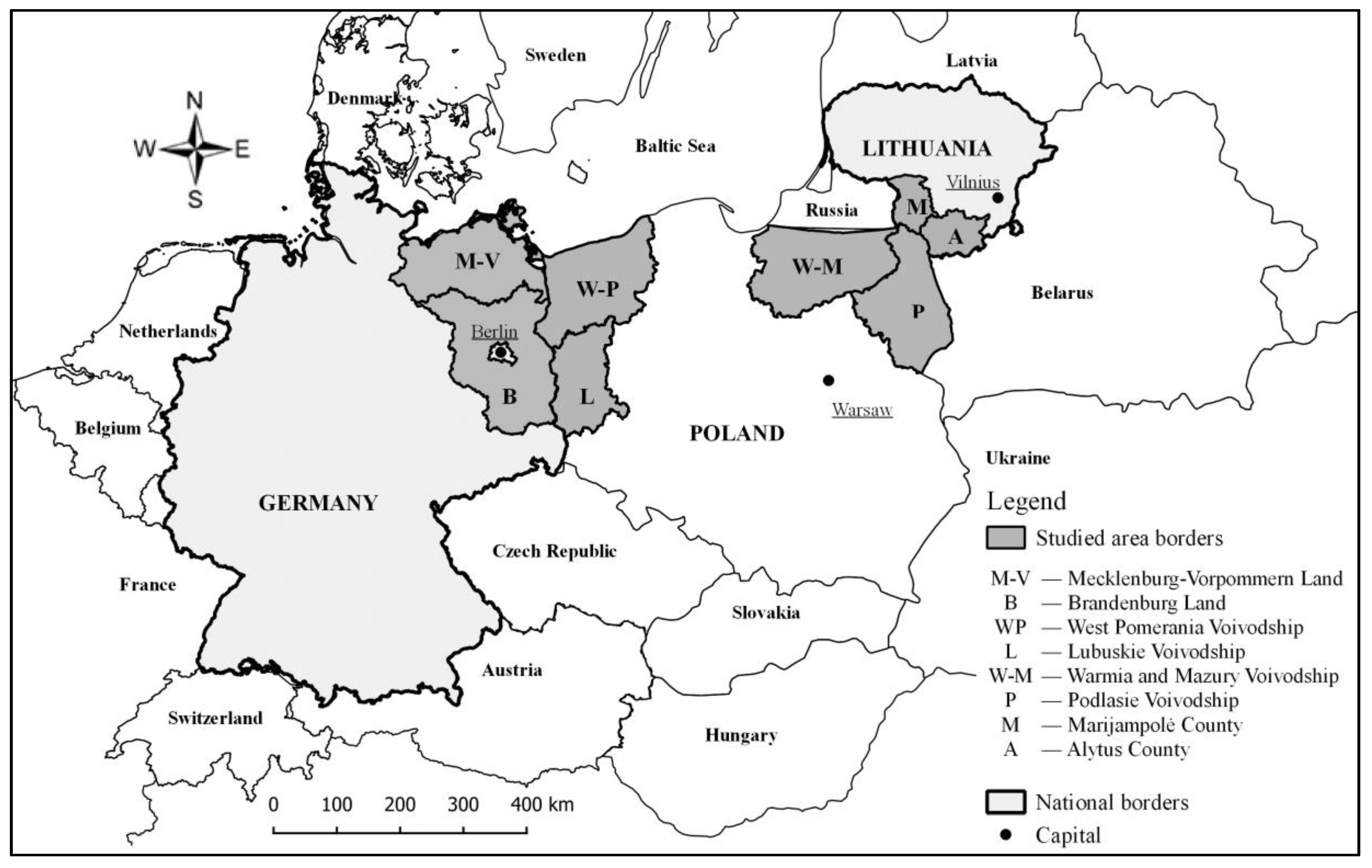
2.1. Study Area

The study area is located in the European Union along Polish–German and Polish–Lithuanian borders and covered: German states—Brandenburg and Mecklenburg-Vorpommern; four Polish voivodeships—West Pomerania, Lubuskie (western Poland, bordering Germany), Warmia and Mazury, and Podlasie (eastern Poland, bordering Lithuania); and two Lithuanian counties—Marijampolė and Alytus (Figure 1).

The analyzed areas are located on the Polish–German and Polish–Lithuanian border, which share a common peripheral location in relation to state borders and central cities. However, an essential role in shaping the demographic potential is also played by the location against the EU border. Therefore, the results of the analyses conducted in the selected transborder regions were interpreted in reference to each country (transborder regions) or the location of the analyzed areas relative to EU borders (internal EU border (A)—Polish–German transborder region and external EU border, (B)—Polish–Lithuanian transborder region) [4,16,26].

The terms used in this study are defined in

Table 1. Definition of the terms used in the study. Source: own elaboration based on administrative divisions.

Term	Definition								Total Number
Study area	Combined data for Polish–German and Polish–Lithuanian transborder regions								2
Transborder regions	Combined data for the areas situated on both sides of the Polish–German border, i.e., the Polish–German transborder region, internal EU border (A)				Combined data for the areas situated on both sides of the Polish–Lithuanian border, i.e., the Polish–Lithuanian transborder region, external EU border (B)				2
NUTS 0	Average data at country level—Germany		Average data at country level—Poland				Average data at country level—Lithuania		3
Border regions	Border region in Germany		Border region in western Poland		Border region in eastern Poland		Border region in Lithuania		4
	Combined data for NUTS 2 units (states): —Brandenburg, —Mecklenburg-Vorpommern		Combined data for NUTS 2 units (voivodeships): —West Pomerania, —Lubuskie		Combined data for NUTS 2 units (voivodeships): —Warmia and Mazury —Podlasie		Combined data for NUTS 2 units (counties): —Alytus —Marijampolė		8
LAU 1	T	26	T	35	T	38	T	10	109
	U	2	U	5	U	5	U	1	13
	R	24	R	30	R	33	R	9	96

T—total number of units, U—number of urban units, R—number of rural units.

.

The analyses of the results at LAU 1 level (Local Administrative Units) provided valuable information about the spatial differentiation of border areas (Figure 2).

The choice of indicators supporting the achievement of the research goal was limited by the availability of demographic data in the national statistical systems of Poland, Germany, and Lithuania. An incredibly difficult task was the selection of indicators at the LAU 1 level. Nevertheless, the authors undertook this task, which allowed for the implementation of the adopted research problem. The statistical data for the analyzed regions had been last updated on 31 December 2017 (Poland and Germany) and 1 January 2018 (Lithuania). Population dynamics were investigated between 2007 and 2017 in Poland and Germany, and between 2008 and 2018 in Lithuania. The choice of 2007 as a starting point was related to the accession of Poland and Lithuania to the Schengen area, which significantly influenced the intensity of population migration with a consequence for the demographic potential.

2.2. Determinants of the Selection of the Research Area

2.2.1. Historical Impact of Demographic Changes

Contemporary demographic phenomena in Polish–German and Polish–Lithuanian transborder areas are rooted in historical processes and changes in the national borders of Central-Eastern European countries after 1945, which had led to mass migration. Migration processes modified the age–sex structure of local communities and led to changes in the proportions of social groups with different educational status. Most immigrants were very young, and the share of resettlers older than 30 was very low, which considerably decreased the mean age of local populations. The loss of men younger than 40 during the war also directly contributed to changes in the age structure of the population. Also, these processes altered the ethnic composition and social structure of Central-Eastern European countries after World War II [42].

In the German states of Mecklenburg-Vorpommern and Brandenburg, which were a part of the Soviet Occupation Zone (SOZ) after World War II, the immigrant population induced significant social changes and exerted a strong influence on the domestic and foreign policy of the former German Democratic Republic (GDR). Mecklenburg was colonized mainly by immigrants from Pomerania, Saxony experienced an influx of immigrants from Silesia, whereas Germans residing east of the Oder and Lusatian Neisse settled in Brandenburg [43]. The resettlement processes in Mecklenburg and Brandenburg were closely related to the existence of a single nation state before World War II, whereas in Poland, the situation was completely different, in particular in the Recovered Territories. These territories were regained by Poland after the war, and they included the present voivodeships of West Pomerania, Lubuskie, and Warmia and Mazury. The cultural heritage of these regions was largely shaped by their political history. The history of Pomerania, Lubusz Land, and Warmia and Mazury is permeated by both Polish and German influences. Local communities and German settlers lived side by side, and their customs and cultures became amalgamated over time. These regions abound in relics of material and spiritual culture that reflect multinational influences. The resettlement of Poles in the Recovered Territories led to considerable changes in the local populations’ geographic and social origins, in particular in early years of the campaign [44]. The new settlers were ethnic Poles who spoke the same language, but they differed in the professed social and cultural values, customs, and aspirations [45]. The transferred Polish nationals were the former inhabitants of Vilnius and Novogrudok regions in the Kresy (Eastern Borderlands) macroregion, which was annexed by the Soviet Union after the war; repatriates who had been exiled to other countries during the war; and settlers from central Poland. Podlasie is the voivodship that belonged to Poland before the war, (therefore, the migration processes in this area were of less importance).

After World War II, mass migration processes also took place in Lithuanian regions situated along the Polish border. Before the war, these areas were a part of Poland, and the Polish inhabitants of Vilnius and Grodno regions in the Kresy macroregion (annexed by the Soviet Union after 1945) accounted for a large part of the immigration wave to Poland. The ethnic and national mosaic of Lithuania was additionally diversified when Lithuania became a Soviet republic after World War II. The country regained independence only in 1991, which was important in shaping the ethnic composition of the population. At the beginning of 2018, Lithuanians were the main ethnic group (86.8%), followed by Poles (5.6%), Russians (4.5%), and other groups (3.1%) [46].

Demographic processes and phenomena in eastern Germany, were also significantly influenced by the mass immigration that followed the fall of the Berlin wall on 9 November 1989. West Germans migrated mostly to East Berlin and rural areas in Brandenburg in the vicinity of Berlin, Potsdam, and Magdeburg. The movement of Germany’s capital from Bonn to Berlin further contributed to West–East migration. The transfer of politicians, experts, and entrepreneurs accelerated the economic development of eastern German regions [47,48]. However, although the relationship between the influx and outflow of people between West and East Germany was two-way, the German border areas with Poland did not enjoy much interest.

Historical processes induce differences in demographic and economic growth [4,49]. The changes in the European borders after World War II caused mass migration, which significantly influenced the sex–age structure of the European population. The attachment to one’s place of residence or birth and the development of “roots” will play an important role in future demographic processes [50]. After World War II, immigrants accounted for a large percentage of the population in the analyzed transborder areas. Resettlers and repatriates were not attached to their new place of residence through birth or upbringing, or through social, occupational, and cultural associations. These factors influenced the demographic potential of the studied areas in the following decades [47].

2.2.2. Natural Values

Both Polish–German and Polish–Lithuanian transborder regions are located in the Central European Plain, in the belt of the South Baltic Lake District (Polish–German) and the Eastern Baltic Lake District (Polish–Lithuanian) [51], which show high natural value and good predisposition for the development of agricultural and touristic functions. The following zones extend in Polish–German and Polish–Lithuanian transborder regions: a lowland zone, a young glacial zone with lively relief, well-defined lines of terminal moraines, outwash plains, numerous lakes and river ice-marginal valleys, and the zone of lake plateaus cut by broad outwash valleys. Within the plateaus, there is a flat and undulating ground moraine, made of glacial till and sandy loam formations. The Baltic coast zone additionally distinguishes Polish–German transborder regions with numerous beaches and chalk cliffs. In Polish–Lithuanian transborder regions, the regions of Warmia and Mazury and Podlasie are characterized by a very diverse landform, with a high share of forests and water bodies. Agricultural land occupies more than half of the region’s territory, and the local economy is based heavily on agriculture [26].

The Lithuanian county of Marijampolė is characterized by a predominance of productive flat land or rolling clayey lowland. Hills and lakes are encountered only in the southern part of the county. Marijampolė has one of the lowest percentages of forest cover in Lithuania. The county Alytus is characterized by the highest degree of naturalness relative to other parts of Lithuania, and it features mostly unproductive sandy plains, lakes, hills, and pine forests [26,52,53].

Moreover, due to the fact that during the socialist period, Poland, Lithuania, and the eastern federal states of Germany belonged to the “eastern states” bloc, they implemented the socialist economic model in various ways.

2.3. Methods

Various definitions of demographic potential exist in the literature. According to Zdrojewski (1995) [54], Szymańska and Biegańska (2010) [55], Rosner (2012) [30], and Rosner and Stanny (2014) [56], demographic potential is described by population size, population density, and population structure based on age and sex, and it is determined by natural population increase and net migration (components of real growth). The age–sex structure of a population is a cumulative result of fertility, mortality, immigration, and emigration [57,58,59,60,61,62]. In a broader sense, it also accounts for education and occupational structure [63,64]. This study was undertaken to investigate quantitative demographic potential, which is defined by rate of changes in population size, population distribution, and population structure by age and sex. Demographic potential is influenced by natural increases and net migration, which are the key components of real growth. It was the basis of the research course carried out covering two aspects influencing the demographic potential, presented schematically in Figure 3. First, a diagnosis of the state of quantitative demographic potential was carried out on the basis of indicators described by population size, population density, and population structure based on age and sex (see Stage 1, Stage 2, Stage 3), and then how natural increase and migration affect quantitative demographic potential (see Stage 4). The relation between the level of the quantitative demographic potential and the strength of the impact on its size by the natural increase and the migration balance was of significant importance for the obtained result, illustrating the quantitative demographic potential (see Stage 5).

The research was conducted in several stages:

2.3.1. Stage 1. Selection of Diagnostic Indicators

Quantitative demographic potential was defined with the use of the diagnostic criteria listed in Appendix A, which were selected based on an analysis of the literature [7,14,30,55,56]. At the same time, as mentioned earlier, the assessment of demographic potential was presented in two versions: as indicators of demographic potential described by population size, population density, and population structure based on age and sex, (see Figure 3) and as indicators determining demographic potential by natural population increase and net migration (components of real growth) by typology by Webb (see Figure 3). The selection of the indicator was made assuming that each indicator could be selected from a given group of issues only once: in indicators that described quantitative demographic potential or in indicators that determined quantitative demographic potential (see Appendix A and

Table 2. Accepted indicators for describing and determining quantitative demographic potential. Source: own elaboration.

Indicator	Name	Description	Type
Quantitative demographic potential is described by indicators:
x1	Population density	Population per unit area (1 km2).	Stimulant
x2	Population dynamics	Changes in the population of Poland and Germany between 2007 and 2017 (as of 31 December 2017) and the population of Lithuania between 2008 and 2018 (as of 1 January 2018). The baseline value (for 2007 and 2008) was set at 100 points, and the values for 2017 and 2018 were calculated relative to the baseline value. Values below 100 are indicative of population decrease, whereas values above 100 are indicative of population increase in the analyzed period.	Stimulant
x3	Proportion of population aged 65 and older in total population (%)	Percentage of the population aged 65 years and older in total population. This is the main indicator of population ageing.	Destimulant
x4	Ageing index	Ratio of the population aged 65 and older to the population aged 0 to 14 * × 100. This indicator provides information about the future potential of young people relevant to seniors.	Destimulant
x5	Femininity ratio	Number of women per 100 men in a given area, which provides information about the reproductive potential of a population	Stimulant
Quantitative demographic potential is determined by indicators:
x6	Natural increase per 1000 population	The difference between the number of live births and the number of deaths in a given area per 1000 population	Stimulant
x7	Net migration per 1000 population	The difference between the inflow and outflow of people to a given area per 1000 population	Stimulant

* 0–15 years for Lithuania.

).

Diagnostic indicators were chosen on the assumption that they should objectively reflect quantitative demographic potential, which is influenced by demographic processes (see Table 2). However, the choice of indicators was limited by the availability and comparability of data at LAU 1 levels in the national statistical systems of Poland, Germany, and Lithuania. To compare the situation against the country and regions (reference point), data at the NUTS 0 and NUTS 2 levels were used.

2.3.2. Stage 2. Statistical Analysis of Selected Indicators

An analysis of the correlations between potential indicators plays an important role during the selection of diagnostic indicators. The chosen indicators for described quantitative demographic potential should be bound by weak mutual correlations [65]. The indicators were statistically validated in an analysis of the diagonal elements of the inverse correlation matrix. Highly correlated variables whose value exceeded 10 in the main diagonal of the matrix were eliminated from further analysis [66]. The selected indicators were arranged in a decision matrix X_mxn, where rows represent the analyzed objects, and columns represent diagnostic indicators (indicators of demographic potential), i.e., x_ij is the value of the jth indicator (j = 1, …, m) of an ith object (i = 1, …, n).

2.3.3. Stage 3. Evaluation of Quantitative Demographic Potential Based on Its Constituent Elements (NUTS 0, NUTS 2, LAU 1) and in a Synthetic Approach (LAU 1)

Analysis of Quantitative Demographic Potential Based on Its Constituent Elements—NUTS 0 and NUTS 2 Levels

The diagnostic indicators presented in Table 2 were used to analyze quantitative demographic potential based on its constituent elements. The analysis was conducted at NUTS 2 level according to the nomenclature described in Table 1.

Border regions are often characterized by adverse demographic trends relative to other parts of the country; therefore, the average values of diagnostic indicators at NUTS 0 (national) level in Poland, Germany, and Lithuania were included in the evaluation.

Analysis of Quantitative Demographic Potential Based on Its Constituent Elements and in a Synthetic Approach at LAU 1 Units

• Determination of synthetic indices for evaluating quantitative demographic potential

Demographic potential is a complex concept that is described with the use of various indicators. In this study, the zeroed unitarization method was used to identify LAU 1 unit with varied demographic potential in quantitative terms. This method enables the substitution of several diagnostic indicators with a single synthetic index. The diagnostic indicators selected in Stage 2 were used to develop a synthetic index for LAU 1 units. Diagnostic indicators were divided into stimulants, which promote the investigated phenomena, as well as destimulants, which detract from the analyzed processes. Diagnostic indicators are often expressed in different units, and they cannot be directly compared and summed up. Therefore, these indicators were normalized and adjusted for comparability by removing the respective units of measurement. This was accomplished with the use of the zeroed unitarization method, where the following transformation operations were applied [67,68]:

For stimulants:

$$v_{ij}=\frac{x_{ij}-min{x}_{ij}}{max{x}_{ij}-min{x}_{ij}}.$$

(1)

For destimulants:

$$v_{ij}=\frac{min{x}_{ij}-x_{ij}}{max{x}_{ij}-min{x}_{ij}}.$$

(2)

Synthetic index$P_{d_i}$is developed as the arithmetic mean of the normalized values of diagnostic indicators:

$$P_{d_i}=\frac{1}{m}{\displaystyle \sum }_{j=1}^m{v}_{ij}$$

(3)

where:

$P_{d_i}$—synthetic index of demographic potential in quantitative terms;

$x_{ij}$—value of the jth diagnostic indicator of an ith object at LAU 1 units;

$max{x}_{ij}$—maximum value of the jth diagnostic indicator;

$min{x}_{ij }$—minimum value of the jth diagnostic indicator;

$max{x}_{ij}\ne min{x}_{ij}$;

$v_{ij}$—value of the jth normalized indicator of an ith object at LAU 1 units;

i = 1, 2, …, n, n—number of LAU 1 units;

j = 1, 2, …, m, m—number of diagnostic indicators.

As a result, the above indicators were transformed into a single synthetic index describing demographic potential in quantitative terms.

The synthetic index $P_{d_i}$ takes on values in the range of [0, 1]. The closer the value of $P_{d_i}$ is to 1, the higher the demographic potential of object i in terms of diagnostic indicators m.

• Spatial distribution of quantitative demographic potential at LAU 1 units

The spatial distribution of demographic potential was additionally determined in quantitative terms. The analyzed areas units (LAU 1) were arranged in a linear order and divided into four classes by calculating the arithmetic mean and standard deviation of the synthetic index of demographic potential ($P_d)$ [65,69] (

Table 3. Demographic potential classes in quantitative terms. Source: own elaboration.

Class	Identification Criteria	Quantitative Demographic Potential
I	$P_d\ge {\overline{P}}_d+S_{P_d}$	high
II	${\overline{P}}_d\le P_d<{\overline{P}}_d+S_{P_d}$	moderately high
III	${\overline{P}}_d-S_{P_d}\le P_d<{\overline{P}}_d$	moderately low
IV	$P_d<{\overline{P}}_d-S_{P_d}$	low

P_d—synthetic index of demographic potential, ${\overline{P}}_d$—arithmetic mean of the indicator of demographic potential, $S_{P_d}$—standard deviation of the synthetic index of demographic potential.

).

2.3.4. Stage 4. Calculation of Real Growth as a Factor Influencing Quantitative Demographic Potential

Natural increase and net migration were analyzed as factors that influence quantitative demographic potential. Natural increase and migration influence population size and the age–sex structure of a population, and both processes contribute to real growth. Natural increase and net migration can be positive or negative. The influence of natural increase and net migration on real growth in the analyzed areas was investigated with the use of the method proposed by J. W. Webb (1964) [4,31,62,70,71,72,73,74] (

Table 4. Demographic categories based on Webb’s typology. Source: own elaboration.

Category	Real Growth	NI—NM relation
Population growth (PG+)
A	PG+	+NI > −NM	Positive natural increase exceeds negative net migration
B		+NI > +NM	Positive net migration and even higher positive natural increase
C		+NI < +NM	Positive natural increase and even higher positive net migration
D		−NI < +NM	Positive net migration compensates for negative natural increase
Population decline (PG−)
E	PG−	−NI > +NM	Negative natural increase is not compensated by positive net migration
F		−NI > −NM	Negative net migration and even higher negative natural increase
G		−NI < −NM	Negative natural increase and even higher negative net migration
H		+NI < −NM	Negative net migration is not compensated by positive natural increase

PG—real growth; NI—natural increase; NM—net migration.

).

The above procedure was applied to illustrate the combined influence of natural increase and net migration on real growth at LAU 1 units. The results were used to present the spatial distribution of real growth in the study area.

2.3.5. Stage 5. Analysis of the Relationship between the Quantitative Demographic Potential and Real Growth (Natural Increse and Net Migration)

The relationship between the quantitative demographic potential and real growth was determined by cross-referencing quantitative demographic potential with the demographic categories based on Webb’s typology. Quantitative demographic potential was also correlated separately with natural increase and net migration.

3. Results and Discussion

The research questions and the adopted course of action in the methods means that the discussion of the obtained results of empirical research is preceded by the presentation of an explanatory background in the form of a theoretical framework covering the theory of geographical location and theory of urban shrinkage.

3.1. Theoretical Framework

Understanding processes shaping and diversifying the demographic potential required a theoretical foundation and presentation of the specificity of the research area undertaken.

3.1.1. Theory of Geographical Location

The spatial diversity of the demographic potential is significantly affected by location values, i.e., the geographical location of the given unit relative to development centers. It means that the “location rent” of a given unit determines the level of development. Thanks to good transport access, rural areas, using economies of scale and agglomeration, increase the impact on neighboring units. Therefore, a higher level of development is achieved by areas located around larger cities and communication routes, as they generate development impulses for rural areas. As we move away from the center, the level of development decreases [75,76]. The location rent has a positive effect on demographic changes (positive migration balance and favorable age structure of the population are observed). At the opposite end of the system there are areas of economic stagnation, which are not conducive to the process of demographic development, and even become one of its main barriers to development [77]. Areas of stagnation have a low level of social capital, which is very often “drained” by areas of growth. These areas show weak development dynamics and negative social effects of the transformation process [78]. Areas with special demographic problems (depopulation) must be treated with special care by the state.

3.1.2. Theory of Urban Shrinkage

One of the most critical problems in the contemporary development of cities includes demographic changes. The population of numerous urban centers shows a long-term decline. This process is referred to as urban shrinkage and takes various forms. It manifests itself in different ways in the city space in different historical, physical, geographic, and socioeconomic conditions [79,80]. After 1990, urban shrinkage was particularly significant in postcommunist countries (including East Germany, Poland, and Lithuania). Urban shrinkage is a specific interaction between the demographic, social, economic, and spatial structure of the city [81]. The key elements include birth rate, population age structure, and migration. Urban shrinkage is a multidimensional process, the effects of which are essential in spatial planning [82]. Although declining urban populations are commonplace, this does not necessarily mean that urban shrinkage occurs everywhere, at the same time and with the same effects. It is quite the opposite—contemporary research has confirmed that the patterns of urban shrinkage are highly diverse [83].

3.2. The Results of Empirical Research

In line with the adopted aim of the study, the assessment and comparison of the demographic potential for border regions were carried out by examining the next aspects:

• Diagnosing quantitative demographic potential is described by population size, population density, and population structure based on age and sex,
• The impact of natural increase and net migration on quantitative demographic potential,
• Identification of the relationship between the quantitative demographic potential level and the impact of natural increase and migration balance (real growth).

3.2.1. Diagnosing Quantitative Demographic Potential

Diagnostic indicators characterizing quantitative demographic potential were selected in the first step of the research process (Table 1). Indicator x₃ (proportion of population aged 65 and older) was eliminated in the statistical analysis (Stage 2). The final list of diagnostic indicators used in the study is presented in

Table 5. Diagnostic indicators for describing the quantitative demographic potential of Polish–German and Polish–Lithuanian border regions at NUTS 0 and NUTS 2 levels. Source: own elaboration based on [46,84,85].

Specification	Germany	Poland	Lithuanian	Polish–German and Polish–Lithuanian Transborder Regions
				Total	Areas Situated on both Sides of the Polish–German Border, i.e., the Polish–German Transborder Region, Internal EU Border (A)			Areas Situated on both Sides of the Polish–Lithuanian Border, i.e., the Polish–Lithuanian Transborder Region, External EU Border (B)
					Total	Border Region in Germany	Border Region in Western Poland	Total	Border Region in Eastern Poland	Border Region in Lithuania
Population density	231	123	43	60	75	77	74	44	59	29
Population dynamics	101	101	83	94	99	97	101	89	100	78
Ageing index	159	106	131	138	147	188	105	129	102	157
Femininity ratio	103	107	117	106	104	103	106	109	105	113

.

Population size and population distribution, defined based on population density, play the key role in evaluations of quantitative demographic potential. The average population density in the study area was 66 persons/km². Historical events, environmental factors, the level of socioeconomic development, and the geographic location of the evaluated regions undoubtedly contributed to differences in their population density. Population density was higher in Polish–German than in Polish–Lithuanian transborder regions. The corresponding differences were observed in Polish border regions. Population density was highest in border regions in western Poland and lower in border regions in eastern Poland. Clear differences were also noted between average population density at the national level and in border regions. The greatest disproportion was noted in Germany, where population density in border regions was nearly three times lower than the national average. This situation resulted from the outflow of people, mainly young people, to Berlin and West Germany since the reunification of Germany, and due to the limited labor market (dominance of the agricultural function). Demographic trends are particularly negative when areas with low population density are also experiencing population decline. The accumulation of all problems, i.e., the peripheral location and the decline in population, may contribute to the accumulation of unfavorable structures and irreversible economic and social processes. This scenario was noted in the sparsely populated Lithuanian border regions, whose population eased by 28% in the last 10 years. The border regions situated in both western and eastern Poland were least affected by these adverse trends. At the same time, it should be emphasized that the slight decrease in the population in the Polish border area with Germany has resulted from the stabilized economic situation of households, whose income often comes from working in Germany. Even at the beginning of the 1990s, there was a tendency to leave for permanent work in Germany with whole families [4]; now, there is a seasonal or daily movement of commuting to work abroad [86]. From the economic point of view, the ageing index, namely the proportion of the population aged 65 and older to the population aged 0 to 14, plays an important role in evaluations of quantitative demographic potential [54]. The lower the value of the ageing index, the higher the potential level of socioeconomic development. The ageing index was high in German (188) and Lithuanian (159) border regions, and it exceeded the national average noted in these countries. The consequence of these changes is a decrease in revenues in the communes’ budget, and the needs for services are not fully met [2]. In border regions in western and eastern Poland, index values were satisfactory (105 and 102, respectively), and they did not differ considerably from the national average. However, the ageing index was higher in the Polish–German transborder region than in the Polish–Lithuanian transborder region, which indicates that elderly residents account for a larger proportion of the population in Polish and Lithuanian border regions. The process of the population ageing applies to the whole of Germany and is the result of an increase in life expectancy (positive effect) and negative population growth (negative effect). However, the border area, due to its marginal location, gives no hope that an influx of young people and a reversal of trends will occur in the near future. For this reason, great hopes are placed in the influx of people from abroad (the policy of settling foreigners from war zones and creating convenient living conditions for Polish citizens) [87]. The femininity ratio was determined at 106 for the study area. In Polish and German border regions, the above metric approximated the national average of each country. However, the femininity ratio reached the highest values of 113 and 117 in Lithuanian border regions and in Lithuania, respectively. These results point to considerable differences in the quantitative demographic potential of border regions already at NUTS 2 level. The high percentage of women in the Lithuanian border area is the result of the increase in the life expectancy of women (positive effect), increased mortality of men (negative effect), and economic migration, mainly of young men.

The above indicators were then applied at LAU 1 units, and a synthetic index supporting a comprehensive evaluation of differences in quantitative demographic potential was developed with the use of the zero unitarization method. Based on the values of the synthetic index, the analyzed LAU 1 units were divided into four classes, where class I denoted units with the highest quantitative demographic potential, and class IV represented units with the lowest quantitative demographic potential (

Table 6. Classification of the quantitative demographic potential of Polish–German and Polish–Lithuanian transborder regions at LAU 1 units based on the values of the synthetic index. Source: own elaboration based on [46,84,85].

Class		Polish–German and Polish–Lithuanian Transborder Regions
		Total		Areas Situated on both Sides of the Polish–German Border, i.e., the Polish–German Transborder Region, Internal EU Border (A)						Areas Situated on both Sides of the Polish–Lithuanian Border, i.e., the Polish–Lithuanian Transborder Region, External EU Border (B)
				Total		Border Regions in Germany		Border Regions in Western Poland		Total		Border Regions in Eastern Poland		Border Regions in Lithuania
		number	%	number	%	number	%	number	%	number	%	number	%	number	%
I	Pd ≥ 0.2270	12	11.0	6	9.8	1	3.8	5	14.3	6	12.5	6	15.8	0	0.0
II	0.1198 ≤ Pd < 0.2270	55	50.5	31	50.8	2	7.7	29	82.9	24	50.0	22	57.9	2	20.0
III	0.0125 ≤ Pd < 0.1198	24	22.0	12	19.7	11	42.3	1	2.9	12	25.0	9	23.7	3	30.0
IV	Pd < 0.0125	18	16.5	12	19.7	12	46.2	0	0.0	6	12.5	1	2.6	5	50.0
Total		109	100.0	61	100.0	26	100.0	35	100.0	48	100.0	38	100.0	10	100.0

).

The results of the study revealed considerable spatial variation in the quantitative demographic potential of Polish–German and Polish–Lithuanian transborder regions at LAU 1 units (Figure 4). An analysis of LAU 1 units based on the values of the synthetic index produced rather optimistic results because 61.5% of the evaluated units belonged to class I and II, and only 16.5% of the units belonged to class IV. Class I units characterized by high quantitative demographic potential were composed of 12 LAU 1 units, including 9 urban units, mostly regional capitals and cities that act as regional hubs. The remaining three units were situated in the vicinity of cities (Berlin, Szczecin, and Olsztyn). Class I units were attractive places of residence and work because in 8 out of 12 cases, the values of all diagnostic indicators significantly exceeded the average values for the study area at LAU 1 units. Class I units were characterized by high population density, population growth, and a favorable sex–age population structure. These units were situated in Polish–German (50%) and Polish–Lithuanian (50%) transborder regions. Class II contained the smallest number of units, and it was characterized by above-average quantitative demographic potential. Class II was composed mainly of rural units with generally low population density. Despite the above, class II units were characterized by population growth and a favorable sex–age population structure. These units were found in Polish–German (56%) and Polish–Lithuanian (44%) transborder regions, and 93% of them were situated in Poland. Below-average quantitative demographic potential was noted in 24 LAU 1 units belonging to class III. These units were characterized by low population density, population decline, low femininity ratio, and a higher ageing index in comparison with class I and II units, which is indicative of rapid population ageing. Class III units were distributed evenly in Polish–German (50%) and Polish–Lithuanian (50%) transborder regions. The LAU 1 units in class IV were characterized by the lowest quantitative demographic potential due to unfavorable values of the ageing index and population decline. Class IV units accounted for only 16.5% of all LAU 1 units, which should be regarded as an acceptable outcome.

A spatial distribution analysis conducted on LAU 1 units revealed the highest quantitative demographic potential in urban units, regardless of their location in transborder regions (Polish–German or Polish–Lithuanian) or the respective countries. The distribution of LAU 1 units across quantitative demographic potential classes was generally similar in both transborder regions. Polish border regions scored higher in both transborder regions. Some German and Lithuanian border regions were characterized by lower quantitative demographic potential than Polish border regions. These results could be attributed to the fact that border regions in Germany and Lithuania were characterized by a higher population decline and a higher proportion of senior citizens (65 and older) than young dwellers aged 0 to 14 (0 to 15 in Lithuania) in comparison with Polish border regions. However, the severity of these adverse phenomena differed between German and Lithuanian border regions. Population ageing was a greater problem in German border regions (ageing index—188) than in Lithuanian border regions (ageing index—157). In turn, Lithuanian border regions were more affected by population decline (population dynamics in 2008–2018—78 percentage points) than German border regions (population dynamics in 2007–2017—97 percentage points). The results of these studies confirm that the location rent, i.e., the distance to centrally located urban centers, affects the development of the demographic potential. The German border region, in comparison to the Lithuanian one, despite the intensified ageing process, had a more favorable population potential due to the influence of a very strong metropolitan center of Berlin and a dense transport network (road and rail) enabling commuting, including Polish workers. However, compared to the Polish border region, the German demographic potential was weaker. This is mainly due to the lack of interest of the German population for living in the border region.

3.2.2. The Impact of Natural Increase and Net Migration on Quantitative Demographic Potential

An important element shaping the demographic potential is the natural increase and the migration balance.

Natural increase per 1000 population was determined at −3.2, and net migration per 1000 population—at 0.1 for the entire study area. However, differences in the above indicators were noted between the evaluated border regions. Polish–German (internal EU border—B) and Polish–Lithuanian (external EU border—A) transborder regions were characterized by similar natural increase per 1000 per population, but they differed considerably in terms of net migration per 1000 population, which was determined at 2.9 in the Polish–German transborder area and at −2.8 in the Polish–Lithuanian transborder area. Considerable differences in the values of the above parameters were also observed between countries. Natural increase per 1000 population ranged from −0.2 in border regions in eastern Poland to −7.5 in Lithuanian border regions. Net migration per 1000 population was highest in German border regions (6.7) and lowest in Lithuanian border regions (−3.8) (

Table 7. Natural increase and net migration per 1000 population at NUTS 0 and NUTS 2 levels. Source: own elaboration based on [46,84,85].

Specification	Germany	Poland	Lithuanian	Polish–German and Polish–Lithuanian Transborder Regions
				Total	Areas Situated on both Sides of the Polish–German Border, i.e., the Polish–German Transborder Region, Internal EU Border (A)			Areas Situated on both Sides of the Polish–Lithuanian Border, i.e., the Polish–Lithuanian Transborder Region, External EU Border (B)
					Total	Border Region in Germany	Border Region in Western Poland	Total	Border Region in Eastern Poland	Border Region in Lithuania
Natural increase per 1000 population	−1.78	−0.02	−4.07	−3.2	−2.6	−4.7	−0.4	−3.8	−0.2	−7.5
Net migration per 1000 population	5.03	0.04	−1.17	0.1	2.9	6.7	−0.8	−2.8	−1.7	−3.8

).

The processes of integration and the opening of labor markets to employees of the new Member States played a particularly important role in the context of the research. The emigration of people from Poland and Lithuania had an economic basis, and its participants were mainly young people [88,89,90]. This fact exerts a particular influence on the changes in the population age structure and this, in turn, leads directly and gradually to socioeconomic problems [88,89,91,92]. Migration losses that mainly involve young people, known as a brain drain, i.e., the loss of a highly qualified labor force [90,92]. The most attractive Polish, as well as Lithuanian, emigrants were to, in particular, the United Kingdom, Ireland, Germany, Denmark, and Norway [91,92]. It should be emphasized that the accession of Poland and Lithuania to the EU contributed to the free movement of people, including increased economic migration; however, they differed in the scale of this process. Taking in to consideration the migration rate, Lithuania’s rank compared to the other new EU member states is very high. Lithuania needs to deal with the problem of emigration [93]. In Poland, emigration was not as massive as in Lithuania. The neighborhood with Germany, which is a critical labor market for residents of the border voivodeships (Zachodniopomorskie and Lubuskie), contributed to daily, temporary, and permanent labor migration. Permanent migration affected mainly young people who, when moving from the Polish to the German border zone, were guided by the improvement of living conditions, without losing ties with the family they had left behind. Thus, Germany (the old EU member state), with more favorable economic conditions than Poland and Lithuania, became the recipient of young emigrants from these countries. The effect of these processes is the improvement of the migration balance per 1000 population in Germany compared to Polish–Lithuanian transborder regions.

An analysis of the demographic categories based on Webb’s typology and the average values of natural increase and net migration per 1000 population is very important for the demographic development, proving its trends. Webb’s typology is a helpful tool used to study the “shrinkage” of urban centers [73,94].

The entire study area revealed the presence of category E, where negative natural increase is not compensated by positive net migration. However, the values of both components lead to negative real growth. The least favorable scenario is noted in categories F and G, where both natural increase and net migration are negative. This trend was observed in the Polish–Lithuanian transborder region, which was characterized by negative net migration and even higher negative natural increase (category F). A somewhat more positive scenario was noted in the Polish–German transborder region, where positive net migration compensated for negative natural increase (category D). It should also be noted that the relationships between natural increase and net migration were generally similar at NUTS 2 and NUTS 0 levels (national average). The German border region, as well as the entire country (Germany), were placed in category D, whereas the Lithuanian border region and Lithuania were assigned to category F. In contrast, Poland was placed in category D, whereas its western and eastern border regions were assigned to the less favorable category G. At the same time, certain relationships were noted between NUTS 2 and LAU 1 units belonging to different demographic categories based on Webb’s typology (

Table 8. Classification of LAU 1 units based on Webb’s method. Source: own elaboration.

Type	Polish–German and Polish–Lithuanian Transborder Regions
	Total	Areas Situated on both Sides of the Polish–German Border, i.e., the Polish–German Transborder Region, Internal EU Border (A)			Areas Situated on both Sides of the Polish–Lithuanian Border, i.e., the Polish–Lithuanian Transborder Region, External EU Border (B)
		Total	Border Region in Germany	Border Region in Western Poland	Total	Border Region in Eastern Poland	Border Region in Lithuania
A	6	1	-	1	5	5	-
B	1	1	-	1	-	-	-
C	8	6	1	5	2	2	-
D	16	16	15	1	-	-	-
E	10	10	8	2	-	-	-
F	15	3	2	1	12	7	5
G	39	20	-	20	19	14	5
H	14	4	-	4	10	10	-
Total	109	61	26	35	48	38	10

).

The highest number of LAU 1 units—39 (36%)—were allocated to category G characterized by negative natural increase and even higher negative net migration. However, considerable differences were noted between LAU 1 units in the analyzed transborder regions. In the Polish–German transborder region, 39.3% of LAU 1 units were characterized by positive real growth. Most of these units were placed in category D, where positive net migration compensated for negative natural increase. Many units with negative real growth were assigned to category G, characterized by negative natural increase and even higher negative net migration, as well as category E, where negative natural increase was not compensated by positive net migration. Far less favorable trends were observed in the Polish–Lithuanian transborder region, where positive real growth was noted in only 14.6% of LAU 1 units, whereas the remaining 85.4% of LAU 1 units were characterized by negative real growth. It should also be noted that 64.6% of LAU 1 units belonged to categories F and G, with both negative natural increase and negative net migration.

Certain relationships were also observed in the spatial distribution of demographic categories based on Webb’s typology (Figure 5). In the German border region, positive real growth was noted in 61.5% and negative real growth in only 38.5% of LAU 1 units. The highest number of LAU 1 units (57.6%) belonged to category D, where positive net migration compensated for negative natural increase and where positive real growth was noted. The distribution of LAU 1 units characterized by positive and negative real growth was similar in border regions in western and eastern Poland. In western Poland, negative real growth was noted in 77.1% and positive real growth in only 22.9% of LAU 1 units. In eastern Poland, these proportions were determined at 81.6% and 18.4%, respectively. In both western and eastern Poland, the most prevalent demographic category was category G, with negative natural increase and even higher negative net migration. In the Lithuanian border region, real growth was observed in all LAU 1 units (category F—50%, category G—50%), which is the least favorable scenario, where negative natural increase is accompanied by negative net migration. The spatial distribution analysis demonstrated that the relationships between natural increase and net migration were more favorable in the German border region and least favorable in the Lithuanian border region. It should be mentioned, however, that in East Germany, since the beginning of the 1990s, the process of urban shrinkage has been observed, i.e., a long-term decline in the population associated with the crisis of the local economy and growing social problems. This research has confirmed that this process is particularly large in the German border area. In the theory of urban shrinkage, demography related to the decline in population and the unfavorable age structure of the population is of particular importance. On the basis of the conducted research, unfavorable values were recorded for the adopted municipal units in Lithuania, while the process was not so advanced in municipal units in Poland. On the other hand, the adopted level of research did not cover all the cities of the German–Polish border areas and the Polish–Lithuanian border areas. However, the conducted Webb’s typology allowed us to capture a very unfavorable situation, which we dealt with in the studied rural units in border areas in Poland and Lithuania. For the majority of rural units in the Polish border areas and in all the Lithuanian ones, an actual negative increase was recorded, which was influenced by both negative natural growth and negative net migration (type F and type G). This state proves a very unfavorable situation, which may contribute to the deterioration of the demographic potential of these units in the future.

3.2.3. Identification of the Relationship between The Quantitative Demographic Potential Level and the Impact of Natural Increase and Migration Balance (Real Growth)

The associations between quantitative demographic potential level and real growth (determined by the relationships between natural increase and net migration in Webb’s approach) were analyzed in the next stage of the study (

Table 9. Quantitative demographic potential of LAU 1 units based on Webb’s typology of demographic categories. Source: own elaboration.

Parameter		Demographic Categories Based on Webb’s Typology								Total
		A	B	C	D	E	F	G	H
Quantitative demographic potential (classes)	I	5	0	4	0	1	1	1	0	12
	II	1	0	4	3	1	3	30	13	55
	III	0	1	0	10	1	5	6	1	24
	IV	0	0	0	3	7	6	2	0	18
Total		6	1	8	16	10	15	39	14	109

).

An analysis of the quantitative demographic potential of LAU 1 units in view of Webb’s method revealed that quantitative demographic potential was most influenced by net migration in class I and II units, and by natural increase in class III and IV units. So, a relationship was noted between the level of demographic potential and real growth (illustrating the relationship between the natural increase and the migration balance). Among LAU 1 units, characterized by a high demographic potential, as many as 75% had positive real growth (type A, C) and only 25% of units showed negative real growth (type E, F, G). For units classified as class II and III, the relationship between belonging to types with positive and negative real growth was unfavorable. On the other hand, the impact of the natural increase and the migration balance on the quantitative demographic potential for units with a low level (classes IV) was clearly visible. Among LAU 1 units, only 17% had positive real growth (type D), and negative real growth (type E, F, G) was noted for the remaining 83% of units. Particularly disadvantageous is the fact that for 51% of the total of all analyzed units, E and G types were recorded, for which both the natural increase and net migration were negative. That is why the relationships between quantitative demographic potential and natural increase and between quantitative demographic potential and net migration were analyzed in greater detail (

Table 10. Quantitative demographic potential of LAU 1 units based on the relationship between natural increase and net migration per 1000 population. Source: own elaboration.

Parameter		Natural Increase Per 1000 Population	Net Migration Per 1000 Population
		Average Value
Quantitative demographic potential of LAU 1 units (classes)	I	1.3	3.2
	II	−0.8	−2.6
	III	−3.9	0.8
	IV	−7.7	−0.2
Average for the study area		−2.4	−0.8

).

The average values in the evaluated classes were most favorable (positive natural increase and positive net migration) in LAU 1 units with the highest quantitative demographic potential (class I). In turn, the least favorable values (negative natural increase and negative net migration) were noted in class IV as well as class II units. These results can be attributed to negative natural increase and even higher negative net migration in class II, and to negative net migration and even higher negative natural increase in class IV units. On the basis of the performed identification, the determining role was observed between the level of quantitative demographic potential and the natural increase and net migration. In particular, we can see that the higher the demographic potential, the higher the natural increase. Also, for units with high demographic potential (class 1), high positive net migration was recorded. The spatial analysis of demographic potential and demographic types according to Webb shows that units with high demographic potential (class 1) showed a positive birth rate and a positive migration balance for the most part (Figure 4 and Figure 5). On the other hand, the units with the lowest level of demographic potential (class 4) had negative population growth, while net migration was negative for seven units and positive for 10 units.

4. Conclusions

The following conclusions can be formulated based on the presented analysis of the quantitative demographic potential of Polish–German and Polish–Lithuanian transborder regions at NUTS 2 level and LAU 1 units. At the same time, the obtained results were limited by the availability of statistical data for all research areas in terms of the femininity ratio at the age of 20–34 and the number of emigrants aged 20–39 in the total number of emigrants. Their use could have revealed even greater spatial disproportions in the border regions studied. They were replaced with the femininity ratio indicators and migration balance per 1000 population.

The quantitative demographic potential of both NUTS 2 level and LAU 1 units was characterized by considerable spatial variation. Adverse demographic processes, including unfavorable sex–age structure and population decline, were more pronounced in German and Lithuanian border regions than in Polish border regions. It should be emphasized that the border regions of Poland, Lithuania, and Germany showed less favorable indicators describing the demographic potential (described by population size, population density, and population structure based on age and sex) than the corresponding average value for the country. Moreover, the common feature of the examined border regions was negative population growth, below the national average. On the other hand, visible differences were observed in terms of the size of the net migration. For Poland and Lithuania, the recorded negative net migration was below the national average, while for the border region in Germany a positive net migration was noted above the national average. The above research results confirm the theory of the ‘location rent’, that the marginal location in relation to centrally located centers has an impact on shaping the unfavorable demographic potential. In addition, as the research under the adopted approach showed, differences in shaping the demographic potential of border regions related to location against the EU borders; more favorable demographic potential in terms of quantity was noted for the Polish–German transborder region located within the EU than for the Polish–Lithuanian transborder regions located at the external EU border zone.

Special emphasis should be placed on the fact that some border regions in Germany and Lithuania were characterized by lower demographic potential than Polish border regions. In Germany and Lithuania, these observations can be largely attributed to two adverse phenomena: population decline and an unfavorable ratio of the population aged 65 and older to the population aged 0 to 14 (0 to 15 for Lithuania). Population ageing is a more severe problem in Germany than in Lithuania, but it proceeds more rapidly in Lithuania due to a high migration rate among young people. In Germany, population ageing is more advanced and it proceeds less rapidly. The situation in the study area was largely influenced by historical processes, in particular, the movement of national borders in 1945 and mass migration after World War II. In Germany, other important contributors were the collapse of the Berlin wall in 1989, the German unification of 1991, and the continued migration of young people from eastern to western Germany since 1990.

The low quantitative demographic potential of the Lithuanian border region has resulted from population decline caused by mass emigration, in particular among young people (mainly permanent migrations are related to the opening of the labor markets of the European Union). These processes exert a negative influence on the age structure of the population.

The border regions in western and eastern Poland were characterized by higher quantitative demographic potential than the border regions in Germany and Lithuania. Despite progressing population ageing, rural units in Polish border regions remain fairly young. In addition, an important role was played by the volume of migration in border regions in Poland after the opening of labor markets, which was not as large as in the Lithuanian border region. However, comparing the border regions in Poland adopted for the research, the data indicate that higher migration was recorded from the eastern Polish–Lithuanian border region than from the western Polish–German border region. The used data do not take into account circular migrations, which largely concern the inhabitants of the Polish–German border regions.

LAU 1 units with a high quantitative demographic potential (class I) accounted for 11% of all analyzed units, and most of them were urban units and suburban zones of regional cities. The study also revealed that a region’s quantitative demographic potential tended to decrease with an increase in distance from a city. The vast majority of units with the lowest quantitative demographic potential (class IV) were rural units.

Quantitative demographic potential is influenced by natural increase and net migration, and the relationships between these two processes play a particularly important role, determining the actual increment. A thorough knowledge of quantitative demographic potential, natural processes, and migration (the typology of Webb) is required to develop effective regional policies. Webb’s applied typology showed the direction of the changes taking place and the importance of these two factors on the demographic potential. The quantitative demographic potential of class I and II units was more influenced by net migration than by natural increase, whereas the reverse was noted in class III and IV units.

Referring to the theory of “urban shrinkage”, it can be said that this phenomenon is intensifying in the German border regions. The process of shrinking cities, which started after the reunification of Germany, is gaining momentum, mainly due to the outflow of young people to Berlin and West Germany. There are attempts to compensate for population losses in cities by settling foreign nationals in them and creating favorable living conditions for residents of the Polish border zone, e.g., creating Polish–German schools and kindergartens. The adopted level of research for the German–Polish border region, as well as for the Polish–Lithuanian border region, did not allow us to say how advanced this process is in all cities. However, on the basis of the conducted research, unfavorable values were noted for the adopted municipal units in Lithuania, while the process was not so advanced in municipal units in Poland. At the same time, the conducted research allowed us to capture a very unfavorable situation, which we dealt with in the studied rural units in border regions in Poland and Lithuania, where an actual negative real growth was recorded, which was influenced by both negative natural increase and negative net migration. This is a very unfavorable situation, which has and will have an impact on the image of the quantitative demographic potential.

If we focus on the driving forces of demographic processes, it can be stated that soon the demographic potential of Poland and Lithuania will be closer to that of Germany. The scale of this phenomenon will largely depend on the attractiveness of living conditions and the regional policy. In the case of Lithuanian border regions, there were no actions that would stop the migration process that shapes the demographic potential. The consequences of the erroneous regional policy will be felt for a long time in the future. Thus, if no measures are introduced to keep people in Polish border regions, Polish border regions may share the fate of Lithuanian border regions. That is why it is so important to pay attention to the ongoing demographic processes. The later the remedial actions are taken, the more the costs related to the improvement of the demographic situation may be disproportionate to the achieved results. This problem already requires concrete measures to be taken before there are irreversible consequences for their demographic structures in border regions. In Germany, even though remedial measures were taken quickly to stop the unfavorable demographic processes, positive demographic changes are still to come.

In the future, it can be expected that the less favorable development of the population will continue, e.g., as a result of an ageing population. Bearing in mind that border regions, due to their marginal location, are limited in terms of social and economic development, the only chance for their development is a balanced demographic potential. At the same time, depopulation areas with a poor financial condition should create necessary public services within the framework of transborder cooperation (intercommune, civic involvement) in the area of Euroregions.

Otherwise, the accumulation of all the problems, i.e., structural weaknesses, peripheral location, and population decline, may contribute to the accumulation of unfavorable structures and irreversible economic and social trends. The area with a strong demographic structure has much better opportunities for socioeconomic development.

References

1. Bußmann, A. Die Dezentrale Grenzüberschreitende Zusammenarbeit mit Deutschlands Nachbarländern Frankreich und Polen; Nomos Verlagsgesellschaft: Baden-Baden, Germany, 2005; ISBN 978-3-8329-1229-1. [Google Scholar]
2. Maretzke, S.; Porsche, L. (Eds.) Kleinstädte in ländlichen Räumen. Ein Spiegelbild ihrer ökonomischen, sozialen und siedlungsstrukturellen Rahmenbedingungen. In Das Neue Wachstum der Städte. Ist Schrumpfung jetzt Abgesagt? BBSR: Berlin, Germany, 2020; pp. 36–55. ISBN 1868-0097. [Google Scholar]
3. Porsche, L. Die Zukunft von Kleinstädten gestalten. Entwicklungsperspektiven für Kleinstädte eröffnen. Raum Plan. 2015, 181, 26–33. [Google Scholar]
4. Jezierska-Thöle, A. Rozwój obszarów wiejskich Polski Północnej i Zachodniej oraz Niemiec Wschodnich; Wydawnictwo Naukowe Uniwersytetu Mikołaja Kopernika: Toruń, Poland, 2018; ISBN 978-83-231-3881-5. [Google Scholar]
5. Krüger, A. Nachhaltiges Suburbia?—Umdeutungen der Raumbezüge für Kleinstädte mit Leerstands phänomenen in der Nähe von ostdeutschen Wachstumskernen in der Peripherie am Beispiel des Saaletals. In Wohnungsleerstände in Deutschland; Schmidt, H., Vollmer, M., Eds.; Wüstenrotstiftung: Darmstadt, Germany, 2017; pp. 297–317. [Google Scholar]
6. Dannenberg, P.; Lang, T.; Lehmann, K. Einführung “Ländliche Räume” in Deutschland: Neuere Zugänge zu einer alten Kategorie. Eur. Reg. 2012, 18, 55–59. [Google Scholar]
7. Kołodziejczyk, D. Ocena potencjału demograficznego gmin w Polsce (w aspekcie ilościowym i jakościowym). Studia Obsz. Wiej. 2002, 2, 19–30. [Google Scholar]
8. Sudra, P. Ocena potencjału demograficznego wybranych gmin położonych w rejonie węzłów autostrady A2. Człowiek Środowisko 2015, 39, 71–93. [Google Scholar]
9. Morosanu, L. Professional bridges: Migrants’ ties with natives and occupational advancement. Sociol. J. Br. Sociol. Assoc. 2016, 50, 349–365. [Google Scholar] [CrossRef]
10. Bundesamt für Migration und Flüchtlinge Forschungszentrum. Wanderungsmonitoring: Erwerbsmigration nach Deutschland. Jahresbericht 2015; Migration, Integration und Asyl: Berlin, Germany, 2016. [Google Scholar]
11. Siedentop, S.; Uphues, N. Ländliche Räume im Sog der Reurbanisierung? Befunde für Baden-Württemberg und raumordnungs-politische Schlussfolgerungen. In Reurbanisierung in Baden—Württembergischen Stadtregionen; Fricke, A., Siedentop, S., Zakrzewski, P., Eds.; Akademie für Raumforschung und Landesplanung: Hannover, Germany, 2015; pp. 187–203. [Google Scholar]
12. Schäfer, H. Arbeitsmarkt: Arbeitsangebot und Arbeitsvolumen. In Perspektive 2035. Wirtschaftspolitik für Wachstum und Wohlstand in der alternden Gesellschaft; Institut der Deutschen Wirtschaft Köln: Köln, Germany, 2017; pp. 58–73. ISBN 978-3-602-14982-7. [Google Scholar]
13. Parysek, J.J. Miasta polskie na przełomie XX i XXI wieku. Rozwój i przekształcenia strukturalne; Bogucki Wydawnictwo Naukowe: Poznań, Poland, 2005; ISBN 83-60247-08-0. [Google Scholar]
14. Stanny, M. Przestrzenne zróżnicowanie rozwoju obszarów wiejskich w Polsce; Instytut Rozwoju Wsi i Rolnictwa Polskiej Akademii Nauk: Warszawa, Poland, 2013; ISBN 978-83-89900-53-1. [Google Scholar]
15. Piracha, M.; Saraogi, A. Remittances and migration intentions of the left-behind. Migr. Dev. 2017, 6, 102–122. [Google Scholar] [CrossRef]
16. Scharr, F.; Aumüller, A.; Barczyk, R.; Riedel, J.; Untiedt, G. Grenzüberschreitende Unternehmensaktivitäten in der sächsisch-polnischen Grenzregion: Gutachten im Auftrag des Bundesministeriums für Wirtschaft und Technologie, mit Unterstützung der Sächsischen Staatsregierung und der Europäischen Union; Ifo Institute—Leibniz Institute for Economic Research at the University of Munich: Monachium, Germany, 2001; ISBN 3-88512-391-6. [Google Scholar]
17. Węcławowicz, G.; Degórski, M.; Komornicki, T.; Korzeń, J.; Bański, J.; Juliusz, K.; Soja, R.; Śleszyński, P.; Więckowski, M. Studia nad Przestrzennym Zagospodarowaniem Obszaru Wzdłuż Granicy Polsko-Niemieckiej (Studies on Spatial Development of the Polish-German Border Region); IGiPZ PAN: Warszawa, Poland, 2006; ISBN 83-87954-86-1. [Google Scholar]
18. Bański, J.; Dobrowolski, J.; Flaga, M.; Janicki, W.; Wesołowska, M. Wpływ Granicy Państwowej na Kierunki Rozwoju Społeczno-Gospodarczego Wschodniej Części Województwa Lubelskiego; PAN. IGiPZ: Warszawa, Poland, 2010; ISBN 978-83-62089-01-7. [Google Scholar]
19. Gwiaździńska-Goraj, M. Przemiany cech demograficznych ludności w latach 1988–2009 i ich wpływ na peryferyzację obszarów wiejskich województwa warmińsko-mazurskiego. Studia Obsz. Wiej. 2011, 26, 153–174. [Google Scholar]
20. Malkowski, A. Regiony przygraniczne jako terytoria peryferyjne na przykładzie wschodniego i zachodniego pogranicza. Pr. Nauk. Uniw. Ekon. We Wrocławiu 2011, 221, 364–372. [Google Scholar]
21. Miszczuk, A. Demograficzne uwarunkowania peryferyjności regionu (na przykładzie Polski Wschodniej). Pr. Nauk. Uniw. Ekon. We Wrocławiu 2011, 168, 472–484. [Google Scholar]
22. Jezierska-Thöle, A.; Janzen, J. Przemiany demograficzne i gospodarki rolnej w wiejskiej strefie przygranicznej Niemiec i Polski. Acta Sci. Pol. Adm. Locorum 2012, 11, 97–108. [Google Scholar]
23. Miszczuk, A.; Wesołowska, M. Demographic and settlement transformations in peripheral regions (based on the example of eastern Poland). Ann. UMCS Geogr. Geol. Mineral. Petrogr. 2012, 67, 141–151. [Google Scholar] [CrossRef] [Green Version]
24. Gwiaździńska-Goraj, M.; Jezierska-Thöle, A. Peryferyjność obszarów wiejskich województwa warmińsko-mazurskiego a zmiany ludnościowe w latach 1988–2011. Studia Obsz. Wiej. 2013, 34, 175–185. [Google Scholar]
25. Hyll, W.; Schneider, L. Relative deprivation and migration preferences. Econ. Lett. 2014, 122, 334–337. [Google Scholar] [CrossRef]
26. Pawlewicz, K.; Senetra, A.; Gwiazdzinska-Goraj, M.; Krupickaite, D. Differences in the environmental, social and economic development of Polish-Lithuanian trans-border regions. Soc. Indic. Res. 2020, 147, 1015–1038. [Google Scholar] [CrossRef] [Green Version]
27. Rink, D.; Haase, A.; Bernt, M.; Arndt, T.; Ludwig, J. Urban Shrinkage in Leipzig, Germany; Department Urban and Environmental Sociology: Leipzig, Germany, 2011; p. 78. [Google Scholar]
28. Pociūtė-Sereikienė, G.; Baranauskienė, V.; Daugirdas, V. Spatial exclusion in Lithuania: Peripheries as “losers”, metropolitan areas as “winners”. Prz. Geogr. 2019, 91, 5–19. [Google Scholar] [CrossRef]
29. Pociūtė-Sereikienė, G.; Kriaučiūnas, E.; Ubarevičienė, R. Peripheralisation trends in rural territories: The case of Lithuania. Stagec 2014, 116, 122–130. [Google Scholar] [CrossRef] [Green Version]
30. Rosner, A. Zmiany Rozkładu Przestrzennego Zaludnienia Obszarów Wiejskich. Wiejskie Obszary Zmniejszające Zaludnienie i Koncentrujące Ludność Wiejską; Instytut Rozwoju Wsi i Rolnictwa Polskiej Akademii Nauk: Warszawa, Poland, 2012; ISBN 83-89900-48-3. [Google Scholar]
31. Heffner, K. Obszary wiejskie i małe miasta: Czy lokalne centra są potrzebne współczesnej wsi? Studia Ekon. 2016, 279, 11–24. [Google Scholar]
32. Maretzke, S. Demografischer Wandel im ländlichen Raum. So vielfältig wie der Raum, so verschieden die Entwicklung. Inf. Raumentwickl. 2016, 2, 169–187. [Google Scholar]
33. Gans, P.; Siedentop, S. Editorial on the special issue “An international perspective on the processes, patterns, and outcomes of reurbanisation”. Comp. Popul. Stud. 2017, 42, 391–398. [Google Scholar] [CrossRef]
34. Haase, A.; Herfert, G.; Kabisch, S.; Steinführer, A. Reurbanization in east German cities. disP Plan. Rev. 2010, 46, 24–35. [Google Scholar] [CrossRef]
35. Beetz, S. Besonderheiten in der Entwicklung kleiner Städte in ländlichen Räumen. In Kleine Städte in Peripheren Regionen. Prozesse—Teilhabe und Handlungsbefähigung—Integriertes Stadtentwicklungsmanagement; Engel, A., Harteisen, U., Kaschlik, A., Eds.; Dorothea Rohn: Detmold, Germany, 2012; pp. 45–66. ISBN 978-3-939486-68-8. [Google Scholar]
36. Brombach, K.; Jessen, J.; Siedentop, S.; Zakrzewski, P. Demographic patterns of reurbanisation and housing in metropolitan regions in the US and Germany. Comp. Popul. Stud. 2017, 42, 281–318. [Google Scholar] [CrossRef]
37. Ubarevičienė, R.; van Ham, M. Population decline in Lithuania: Who lives in declining regions and who leaves? Reg. Stud. Reg. Sci. 2017, 4, 57–79. [Google Scholar] [CrossRef] [Green Version]
38. Kazlauskiene, E.; Zitkiene, R.; Rakauskiene, O.; Ranceva, O. Demographics in quality of life assessment: Lithuania in EU context. KSI Trans. Knowl. Soc. 2014, 7, 18–22. [Google Scholar]
39. Ubarevičienė, R.; van Ham, M.; Burneika, D. Shrinking regions in a shrinking country: The geography of population decline in Lithuania 2001–2011. Urban Stud. Res. 2016, 2016. Available online: https://www.hindawi.com/journals/usr/2016/5395379/ (accessed on 2 November 2020). [CrossRef]
40. Fihel, A.; Okólski, M. Population decline in the post-communist countries of the European Union. Popul. Soc. 2019, 567, 1–4. [Google Scholar] [CrossRef]
41. Thöle, M.; Jezierska-Thole, A. Life expectancy and mortality rates in Poland and Germany—A comparative analysis. In Proceedings of the 13th International Days of Statistics and Economics, Prague, Czechia, 5–7 September 2019; Loster, T., Pavelka, T., Eds.; 2019; pp. 1537–1547. [Google Scholar]
42. Markiewicz, W. Przeobrażenia społeczne ziem zachodnich. In Ziemie Zachodnie w Granicach Macierzy; Wydawnictwo Poznańskie: Poznań, Poland, 1966; pp. 25–39. [Google Scholar]
43. Steinberg, H.G. Die Bevölkerungsentwicklung in Deutschland im Zweiten Weltkrieg: Mit einem Überblick über die Entwicklung von 1945 bis 1990; Kulturstiftung der Deutschen Vertriebenen: Bonn, Germany, 1991; ISBN 978-3-88557-089-9. [Google Scholar]
44. Lüderitz, J. Lagow im Lebuser Land und Umgebung: Ausflüge östlich der Oder; Bock Kuebler Verlag: Berlin, Germany, 2009; ISBN 978-3-86155-115-7. [Google Scholar]
45. Nowakowski, S. Nowa społeczność na ziemiach zachodnich. Nowe Drogi. 1960, 6, 33–41. [Google Scholar]
46. Statistics Lithuania—Oficialiosios Statistikos Portalas. Available online: https://www.stat.gov.lt/en# (accessed on 31 March 2020).
47. Weiß, W. Mecklenburg-Vorpommern: Brücke zum Norden und Tor zum Osten; mit einem Anhang Fakten—Zahlen —Übersichten; Klett-Perthes: Gotha, Germany, 1996; ISBN 978-3-623-00685-7. [Google Scholar]
48. Weiß, W. Der Ländlichste Raum—Regional-demografische Perspektiven. Probleme von Abwanderungsgebieten mit geringer Bevölkerungsdichte. Landkreis 2002, 72, 15–19. [Google Scholar]
49. Bański, J. Współczesne typologie obszarów wiejskich w Polsce—Przegląd podejść metodologicznych. Przegląd Geogr. 2014, 86, 441–470. [Google Scholar] [CrossRef]
50. Rostow, W.W. Theorists of Economic Growth from David Hume to the Present. With a Perspective on the Next Century; Oxford University Press: New York, NY, USA, 1990; ISBN 978-0-19-535979-4. [Google Scholar]
51. Kondracki, J. Geografia Polski: Mezoregiony Fizyczno-Geograficzne; Wydaw. Naukowe PWN: Warszawa, Poland, 1994; ISBN 978-83-01-16022-7. [Google Scholar]
52. Maèiulyt, J.; Veteikis, D.; Sabanovas, S. Recomposition of rural space in Lithuania since the restoration of independence. Acta Sci. Pol. Adm. Locorum 2012, 11, 167–183. [Google Scholar]
53. Senetra, A.; Szczepanska, A.; Veteikis, D.; Wasilewicz-Pszczolkowska, M.; Simanauskiene, R.; Volungevicius, J. Changes of the land use patterns in Polish and Lithuanian trans-border rural area. Baltica 2013, 26, 157–168. [Google Scholar] [CrossRef] [Green Version]
54. Zdrojewski, E.Z. Podstawy Demografii; Wydaw. Uczelniane WSI: Koszalin, Poland, 1995; ISBN 83-86123-21-4. [Google Scholar]
55. Szymańska, D.; Biegańska, J. Potencjał demograficzny. In Charakterystyka Obszarów Wiejskich w 2008 r.; Wydział Poligraficzny Urzędu Statystycznego w Olsztynie: Olsztyn, Poland, 2010; pp. 49–54. ISBN 978-83-88130-83-8. [Google Scholar]
56. Rosner, A.; Stanny, M. Monitoring Rozwoju Obszarów Wiejskich. Etap 1. Przestrzenne Zróżnicowanie Poziomu Rozwoju Społeczno-Gospodarczego Obszarów Wiejskich w 2010 Roku; Fundacja Europejski Fundusz Rozwoju Wsi Polskiej; Instytut Rozwoju Wsi i Rolnictwa PAN: Warszawa, Poland, 2014. [Google Scholar]
57. Prát, Š.; Bui, T.M. A Comparison of Ukrainian labor migration in the Czech Republic and Poland. East Eur. Politics Soc. 2018, 32, 767–795. [Google Scholar] [CrossRef]
58. Cattaneo, C. International migration, the brain drain and poverty: A cross-country analysis. World Econ. 2009, 32, 1180–1202. [Google Scholar] [CrossRef]
59. Rabe, B.; Taylor, M.P. Differences in opportunities? Wage, employment and house-price effects on migration. Oxf. Bull. Econ. Stat. 2012, 74, 831–855. [Google Scholar] [CrossRef]
60. Napierała, J. Regionalne aspekty zróżnicowania mobilności Polaków w świetle wyników sondażu. In Współczesne Migracje Zagraniczne Polaków. Aspekty Lokalne i Regionalne; Kaczmarczyk, P., Ed.; Ośrodek Badań nad Migracjami Uniwersytetu Warszawskiego: Warszawa, Poland, 2008; pp. 133–158. ISBN 978-83-923898-0-4. [Google Scholar]
61. Szyszka, M. Zagraniczna migracja zarobkowa jedną ze strategii życiowych młodego pokolenia. Rocz. Nauk Społecznych 2016, 8, 143–164. [Google Scholar] [CrossRef] [Green Version]
62. Gałka, J. Wpływ permanentnych migracji zagranicznych na zmiany regionalnych układów zaludnienia w Polsce. Studia Ekon. Zesz. Nauk. Uniw. Ekon. Katowicach 2017, 309, 95–108. [Google Scholar]
63. Sanderson, W.C.; Scherbov, S. The characteristics approach to the measurement of population aging. Popul. Dev. Rev. 2013, 39, 673–685. [Google Scholar] [CrossRef] [Green Version]
64. Polakowski, M.; Szelewa, D. Poland in the migration chain: Causes and consequences. Transf. Eur. Rev. Labour Res. 2016, 22, 207–218. [Google Scholar] [CrossRef]
65. Wysocki, F. Metody Taksonomiczne w Rozpoznawaniu Typów Ekonomicznych Rolnictwa i Obszarów Wiejskich; Wydawnictwo Uniwersytetu Przyrodniczego w Poznaniu: Poznań, Poland, 2010; ISBN 978-83-7160-583-3. [Google Scholar]
66. Malina, A.; Zeliaś, A. Taksonomiczna analiza przestrzennego zróżnicowania jakości życia ludności w Polsce w 1994 r. Przegląd Stat. 1997, 44, 11–27. [Google Scholar]
67. Kukuła, K. Metoda unitaryzacji zerowanej na tle metod normowania cech diagnostycznych. Acta Sci. Acad. Ostroviensis 1999, 4, 5–31. [Google Scholar]
68. Bąk, I.; Wawrzyniak, K.; Oesterreich, M. The application of statistical methods to identify factors determining employment effectiveness in district labour offices in Poland. Acta Univ. Lodz. Folia Oeconomica 2019, 4, 235–255. [Google Scholar] [CrossRef]
69. Fura, B.; Wang, Q. The level of socioeconomic development of EU countries and the state of ISO 14001 certification. Qual. Quant. 2017, 51, 103–119. [Google Scholar] [CrossRef] [PubMed] [Green Version]
70. Webb, J.W. Ruch naturalny i migracyjny jako składnik przemian ludnościowych. Przegląd Zagr. Lit. Geogr. 1964, 1, 134–138. [Google Scholar]
71. Gwiaździńska-Goraj, M.; Goraj, S. Transformation of Demographic Characteristics of the Rural Population of the Warmia and Mazury Voivodship; University of Economics in Prague: Prague, Czechia, 2015; Volume 34, pp. 498–510. [Google Scholar]
72. Biały, S.; Długosz, Z. Typologia demograficzna krajów Europy wg Webba w latach 2005–2025. Kult. Polityka 2015, 18, 151–164. [Google Scholar]
73. Serafin, P. Zmiany w typologii demograficznej miejskich obszarów funkcjonalnych Polski w latach 2002–2017. Biul. Kom. Przestrz. Zagospod. Kraj. PAN 2018, 272, 328–343. [Google Scholar]
74. Serafin, P. Zmiany w potencjale demograficznym ludności wiejskiej w województwie małopolskim w latach 1996–2006. Zesz. Nauk. Uniw. Ekon. Krakowie 2010, 821, 79–96. [Google Scholar]
75. Courtney, P.; Errington, A. The role of small towns in the local economy and some implications for development policy. Local Econ. 2000, 15, 280–301. [Google Scholar] [CrossRef]
76. Ettlinger, N. Cultural economic geography and a relational and microspace approach to trusts, rationalities, networks, and change in collaborative workplaces. J. Econ. Geogr. 2003, 3, 145–171. [Google Scholar] [CrossRef]
77. Bass, H.H. Ragnar Nurkse’s development theory: Influences and perceptions. In Ragnar Nurkse (1907–2007): Classical Development Economics and its Relevance for Today; Reinert, E., Kregel, J., Kattel, R., Eds.; Anthem Press: London, UK, 2009; pp. 183–202. ISBN 978-1-84331-819-4. [Google Scholar]
78. Churski, P.; Stryjakiewicz, T. New experiences of Polish regional policy in the first years of membership in the European Union. Quaest. Geogr. 2006, 25, 17–28. [Google Scholar]
79. Stryjakiewicz, T.; Ciesiółka, P.; Jaroszewska, E. Urban shrinkage and the post-socialist transformation: The case of Poland. Built Environ. 2012, 38, 196–213. [Google Scholar] [CrossRef]
80. Stryjakiewicz, T.; Jaroszewska, E.; Marcińczak, S.; Ogrodowczyk, A.; Rumpel, P.; Siwek, T.; Slach, O. Współczesny kontekst i podstawy teoretyczno-metodologiczne analizy procesu kurczenia się miast. In Kurczenie się Miast w Europie Środkowo-Wschodniej; Stryjakiewicz, T., Ed.; Bogucki Wydawnictwo Naukowe: Poznań, Poland, 2014; pp. 9–14. ISBN 978-83-7986-024-1. [Google Scholar]
81. Strauss, B.; Biedermann, R. Urban brownfields as temporary habitats: Driving forces for the diversity of phytophagous insects. Ecography 2006, 29, 928–940. [Google Scholar] [CrossRef]
82. Salone, C.; Besana, A. Urban shrinkage. Theoretical reflections and empirical evidence from a Southern European perspective. In Proceedings of the AESOP-ACSP Joint Congress, Dublin, Ireland, 15–19 July 2013. [Google Scholar]
83. Hospers, G.J. Policy responses to Urban shrinkage: From growth thinking to civic engagement. Eur. Plan. Stud. 2014, 22, 1507–1523. [Google Scholar] [CrossRef]
84. Statistics Poland—Local Data Bank. Available online: https://bdl.stat.gov.pl/BDL/ (accessed on 3 October 2020).
85. Federal Statistical Office Germany. Available online: http://www.destatist.de (accessed on 31 March 2020).
86. Lammers, K.; Niebuhr, A.; Polkowski, A.; Stiller, S.; Hildebrandt, A.; Nowicki, M.; Susmarski, P.; Tarkowski, M. Polsko-Niemiecki Obszar Przygraniczny w Roku 2020—Scenariusz Rozwoju i Zalecenia Odnośnie Jego Realizacji; Hamburgisches Welt-Wirtschafts-Archiv (HWWA) (Hamburg Institute of International Economics): Gdańsk, Poland, 2006; p. 77. [Google Scholar]
87. Borella, S. Migrationspolitik in Deutschland und der Europäischen Union. Eine Konstitutionenökonomische Analyse der Wanderung von Arbeitskräften; 1st Ed.; Mohr Siebeck: Tübingen, Germany, 2008; ISBN 978-3-16-149645-5. [Google Scholar]
88. Grabowska-Lusińska, I.; Okólski, M. Migracja z Polski po 1 Maja 2004 r: Jej Intensywność i Kierunki Geograficzne oraz Alokacja Migrantów na Rynkach Pracy Krajów Unii Europejskie; University of Warsaw, Centre of Migration Research (CMR): Warszawa, Poland, 2008. [Google Scholar]
89. Lesińska, M.; Okólski, M.; Slany, K.; Solga, B. Dekada Członkostwa Polski w UE. Społeczne Skutki Emigracji Polaków po 2004 Roku; Wydawnictwa Uniwersytetu Warszawskiego: Warszawa, Poland, 2014; ISBN 978-83-235-1611-8. [Google Scholar]
90. Sipavičienė, A.; Stankuniene, V. The social and economic impact of emigration on Lithuania. In Coping with Emigration in Baltic and East European Countries; OECD Publishing: Paris, France, 2013; pp. 45–64. ISBN 978-92-64-20491-1. [Google Scholar]
91. Godlewska, J. Migracje i Imigranci w Polsce–Skala, Podstawy Prawne, Polityka. Ekspertyza Przygotowana w Ramach Projektu “EAPN Polska—Razem na rzecz Europy Socjalnej”; Fundusz Inicjatyw Obywatelskich: Rybnik, Poland, 2010. [Google Scholar]
92. Ranceva, O.; Rakauskienė, O. Threat of emigration for the socio-economic development of Lithuania. Bus. Manag. Educ. 2013, 11, 77–95. [Google Scholar] [CrossRef]
93. Streimikiene, D.; Bilan, Y.; Jasinskas, E.; Griksaite, R. Migration trends in Lithuania and other new EU member states. Transform. Bus. Econ. 2016, 15, 21–33. [Google Scholar]
94. Musiał-Malago’, M. Kurczenie się miast Polski—Analiza i pomiar zjawiska. Rozw. Reg. Polityka Reg. 2018, 42, 91–102. [Google Scholar]
Figure 1. Location of Polish–German and Polish–Lithuanian transborder regions. Source: own elaboration.
Sustainability 12 09414 g001
Figure 2. Administrative division of the study area at LAU 1 level (Local Administrative Units). Source: own elaboration. (a) A—Polish–German transborder region—internal EU border; (b) B—Polish–Lithuanian transborder region—external EU border.
Sustainability 12 09414 g002
Figure 3. Quantitative demographic potential in two aspects. Source: own elaboration.
Sustainability 12 09414 g003
Figure 4. Spatial variation in the quantitative demographic potential of LAU 1 units. Source: own elaboration. (a) A—Polish–German transborder region—internal EU border; (b) B—Polish–Lithuanian transborder region—external EU border.
Sustainability 12 09414 g004
Figure 5. Spatial distribution of LAU 1 units based on Webb’s typology of demographic categories. Source: own elaboration. (a) A—Polish–German transborder region—internal EU border; (b) B—Polish–Lithuanian transborder region—external EU border.
Sustainability 12 09414 g005