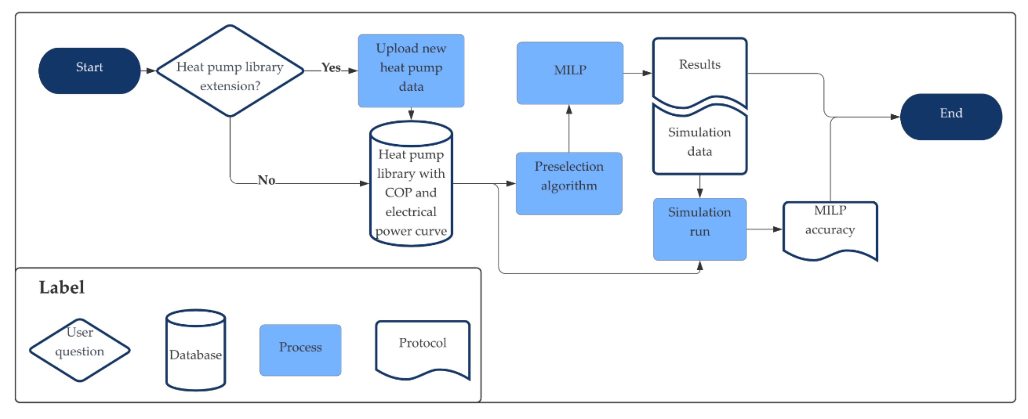
The planning process for the optimal integration of heat pumps is divided into four steps, displayed in
Figure 2. In the first step, a potential library for heat pumps is extended by uploading new heat pump models. The optimization model uses this library, as only existing heat pumps should be considered. The library contains heat pump data in terms of the efficiency curve and electrical power curve. The library is then passed to a preselection algorithm to reduce the computational time of the optimization model. In the third step, the optimization model calculates the optimum constellation of heat pumps and stratified thermal storage tanks for a heating and cooling network to meet respective demand within the optimized operation of one year. The optimization model is formulated as a mathematical model from the problem class MILP consisting of a goal function, a solution space as well as decision variables. As MILP representation, the boundary conditions are formulated linearly while the decision variables can also consist of integer variables. The boundary conditions (here the thermohydraulic system) limit the solution space. The optimization computes the minimum or maximum of the objective function [
11]. The last step is the optional comparison of the MILP results with a simulation model. The simulation model displays the MILP model in the modeling and simulation environment Dymola and is directly connected with the results from the MILP model through a functional mock-up interface (FMI) [
18,
19]. The MILP results are then passed to the user in an Excel sheet containing the configuration of heat pumps and stratified thermal storage tanks as well as their operations at each time step (on/off, heat/cold flow rate).
2.1. Mathematical Model
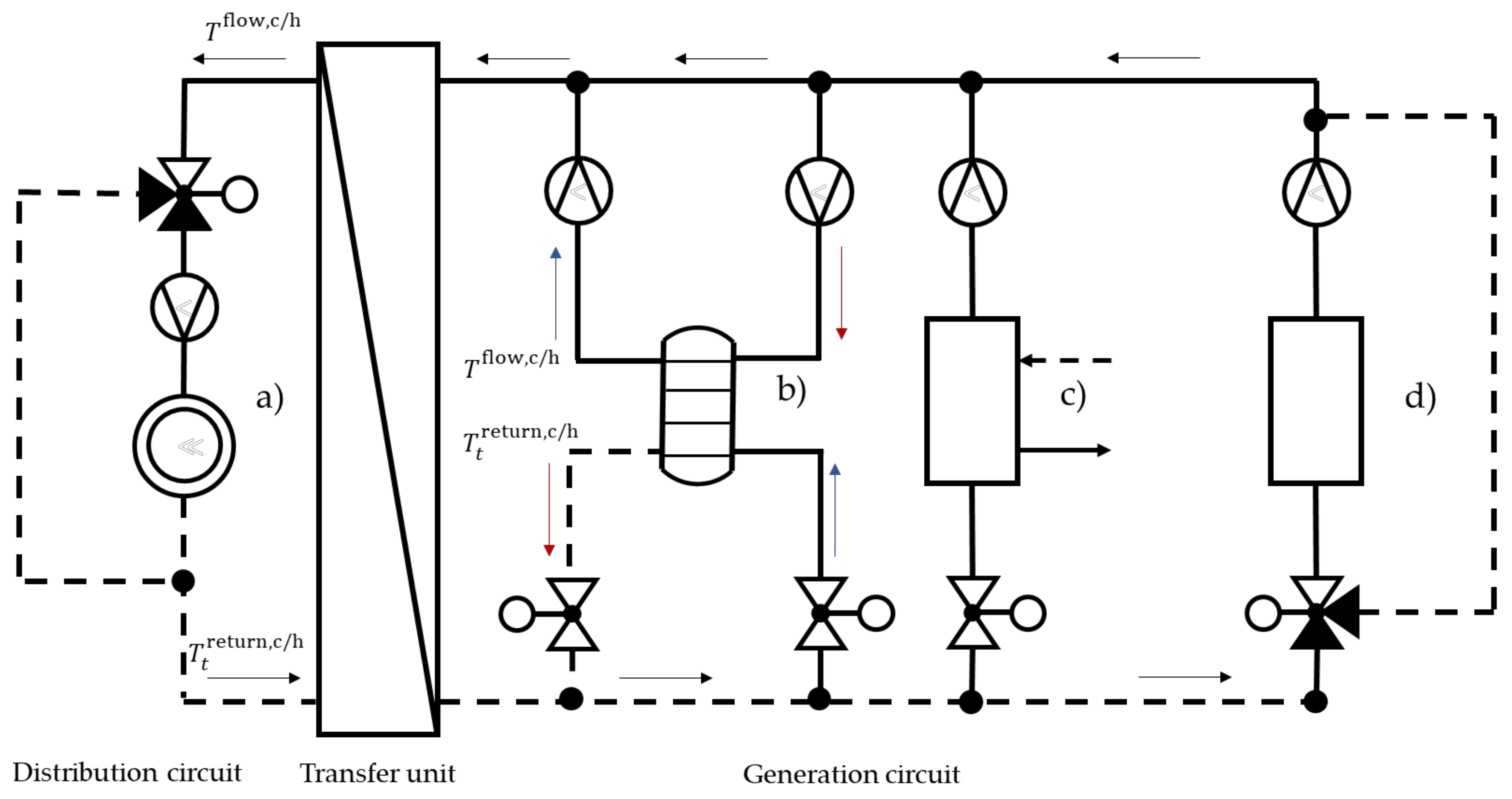
Figure 3 displays a thermohydraulic equivalent circuit of a heating network consisting of a generator circuit (right), a transfer unit (middle), and a distribution circuit (left). Thermal energy is generated by a heat pump (c) and a conventional energy converter (d). The heat pump is connected to a heat source (in this case a cooling network). To offer the heat pump flexibility on the generation side, a stratified thermal storage tank (later referred to as storage) (b) is installed. During the loading process of the storage, a heat rate flows from the flow to the return through the storage layers while the unloading process operates vice versa. The generated energy is transferred through a heat exchanger to the consumer (a).
A MILP model is developed to depict the four components (heat pump, storage, conventional energy converter, consumer) mathematically. All mathematical expressions can be viewed in
Table A5. The model integrates storages and heat pumps into an existing thermohydraulic network consisting of a distribution circuit, transfer unit, and generation circuit with a conventional energy converter. The thermohydraulic equivalent circuit represents the heating and cooling networks, which are modeled analogously to each other. The major assumption of the model is that all energy converters and the storage feed into the network with the same temperature
and receive the same return temperature
from the transfer unit (heat exchanger). However, the storage feed into the flow strand could be lower than
if all layers do not have the flow temperature. This results in a mixing temperature lower than the required demand temperature.
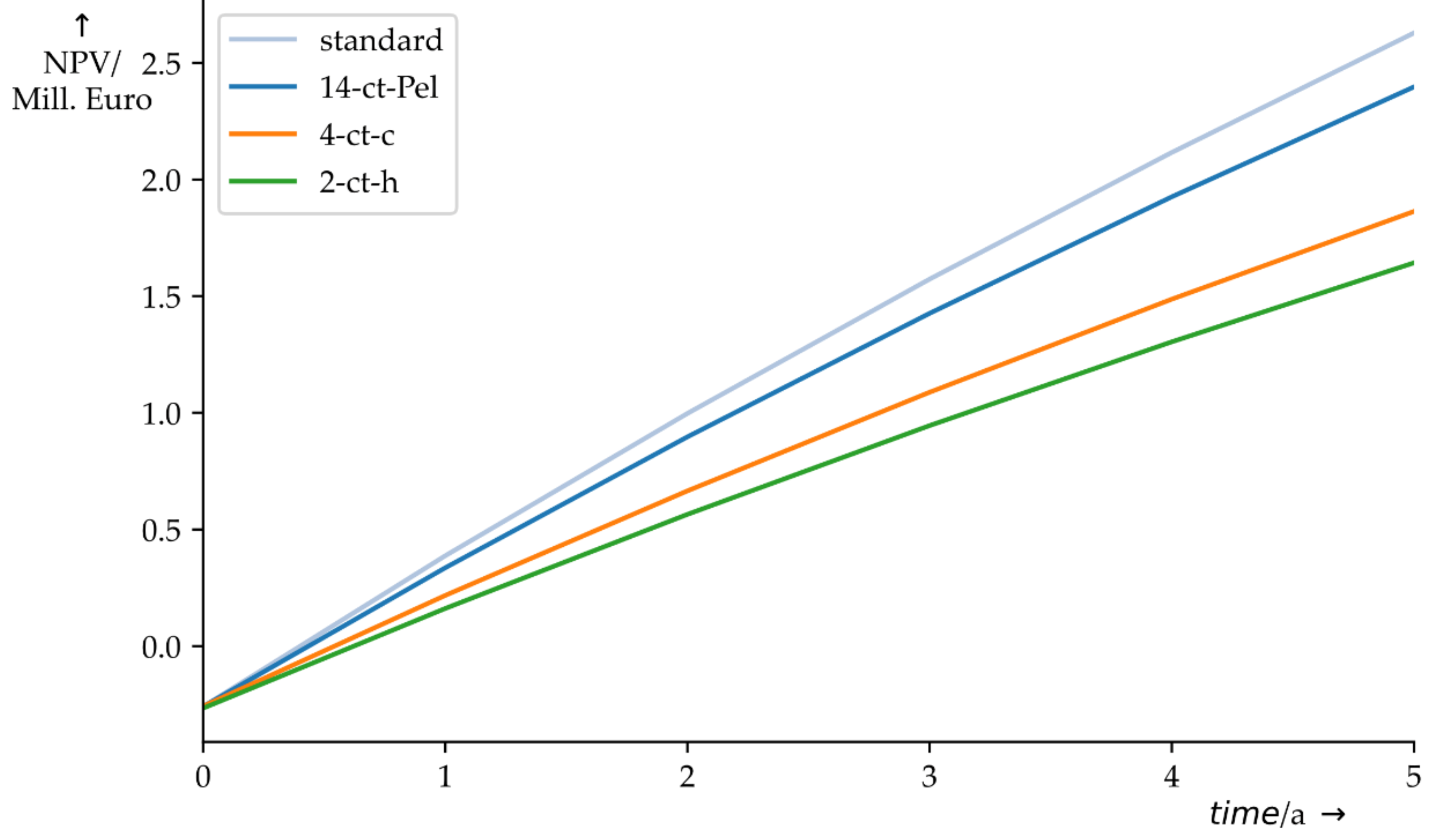
The MILP model seeks the most cost-efficient configuration of heat pumps and flexibility options (storages). The cost-efficient objective is achieved by optimizing the operation of the generation circuit to meet the demand over one year with a temporal resolution of
. The objective function is modeled after the NPV method [
20] (p. 24). The costs are divided into capital expenditures (capex) and operational expenditures (opex). The capex consist of the sum of all heat pump prices
with the buying option
and the storage prices (hot and cold water storage), which are calculated with a volume-specific price of
and the storage dimension (
). The capex do not include investments for conventional energy converters that are assumed to have been integrated into the thermohydraulic network previously. Meanwhile, opex are divided into unoptimized opex and optimized opex. The optimized opex consist of heat pump costs
for electric power
Pi,t, costs for conventional heating
with a heat flow rate
, and costs for conventional cooling
with a cold flow rate
. The unoptimized opex are the operational cost of meeting the heating and cooling demand
with conventional heating and cooling. The profit is calculated by subtracting the optimized opex from the unoptimized opex. The profit is discounted over a payback period
with an interest rate
. To achieve the most cost-efficient configuration, the objective function
must be maximized:
The satisfaction of heating or cooling demand
is ensured by the following condition:
where
is the heat/cold flow rate out of the storage,
is the heat/cold flow rate into the storage, and
is the heat/cold flow rate for every heat pump.
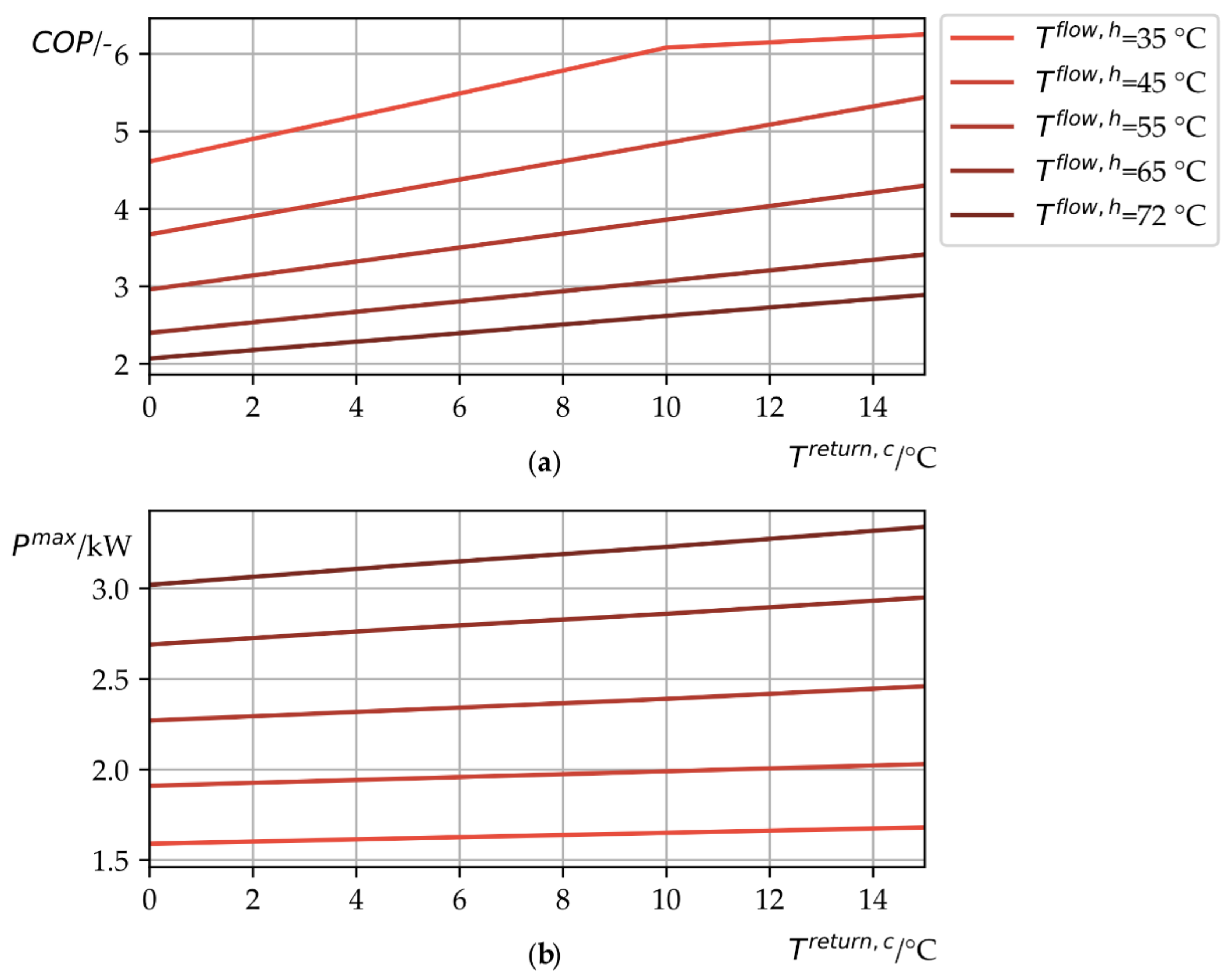
The heat pump is modeled as a quasi-stationary process, and its heat/cold flow rate is calculated with the coefficient of performance (COP) [
21] (pp. 312–314). It is assumed that the temperatures of the network do not change with the integration of the heat pumps and, therefore, are given (assumption is checked in
Section 3.3). The COP and the electrical power curve are then linearized with a multiple linear regression [
22] (pp. 51–53). An example data sheet is provided in
Appendix A (
Figure A1). The COP and the maximum electrical power depend on the flow temperature in the heating circuit and the return temperature in the cooling circuit [
7]. These temperatures are assumed to be given in 15 min time steps over one year. With the regressor functions for every heat pump and the given temperatures at each time step, the
, the maximum electrical power
, and the minimum electrical power
(time independent) can be calculated for one year production prior to the optimization. This results in the linear calculation of the heat flow rate
for every heat pump
i at each time step
t [
21] (pp. 312–314):
The electrical power
of a heat pump,
, can be chosen by the optimizer and is limited by the regressor function for the maximum electrical power
and minimum electrical power
of the heat pump
, with
where
in Equation (5) is the binary buying option and where
in Equation (4) is the binary on-/off-switch for the heat pump. Equation (4) gives the optimizer the flexibility option of partial load by choosing
between the maximum and minimum electrical power feed into the heat pump. The cold flow rate
is calculated analogically to Equation (3) with [
23]:
Every heat pump can be turned on and off to offer the optimizer another flexibility option with the binary variable
. The power circuit of a heat pump should not be interrupted too frequently; therefore, a minimum runtime
is ensured with the following:
The most important element of flexibility in the MILP model is related to storage. The optimizer can choose its dimension freely and is limited only by the space
that the user can offer for hot and cold water storages (
):
The storage loading (marked as a red arrow) and unloading (marked as a blue arrow) in
Figure 3 are modeled as the power flow of an electric battery:
The current state of charge (SOC) is
(current energy level). It is calculated by the sum of SOC from time step
and the heat/cold flow rate
to load the storage over a time step length
. The heat/cold flow rate
to unload the storage over a time step length
is subtracted. The efficiencies for loading and unloading the storage are expressed by
and
. The energy losses of the storage from time step
to
are expressed by multiplying
with an efficiency
. The energy level of the storage is limited by the current return temperature
and the constant flow temperature
:
where
is the density of water and where
is the specific heat capacity of water. The storage is modeled as stratified storage, and these equations follow the assumption that the energy level of the storage is equal to zero if all layers have the return temperature
. The energy level of the storage is at its maximum if all layers have the flow temperature
. Furthermore, it is assumed that the storage unloads and loads always with the flow temperature
. The unloading and loading process is limited according to the following:
where
is the mass flow rate to load or unload the storage. To ensure stable flow conditions during the loading and unloading process, bidirectional flow is forbidden:
where
is a binary variable and
is a Big-M-Coefficient [
11] (p. 219). The binary variable ensures that during the loading process
will be equal to zero because
will be one:
. During the unloading process
will be equal to zero to forbid loading the storage:
. For the Big-M-Coefficient applies
and
, therefore, the loading and unloading process is only limited by Equations (12) and (13).
In addition to the mathematical formulation, it should be noted that all parameters (technical or economic) can be easily changed (e.g., efficiencies, fluid parameters). Although the heat pump library is static, it can also be modified by the user. The model can select from all available heat pumps, which results in an exponential rise of the computational time, and therefore, an algorithm is developed to reduce computational time by preselecting possible options.
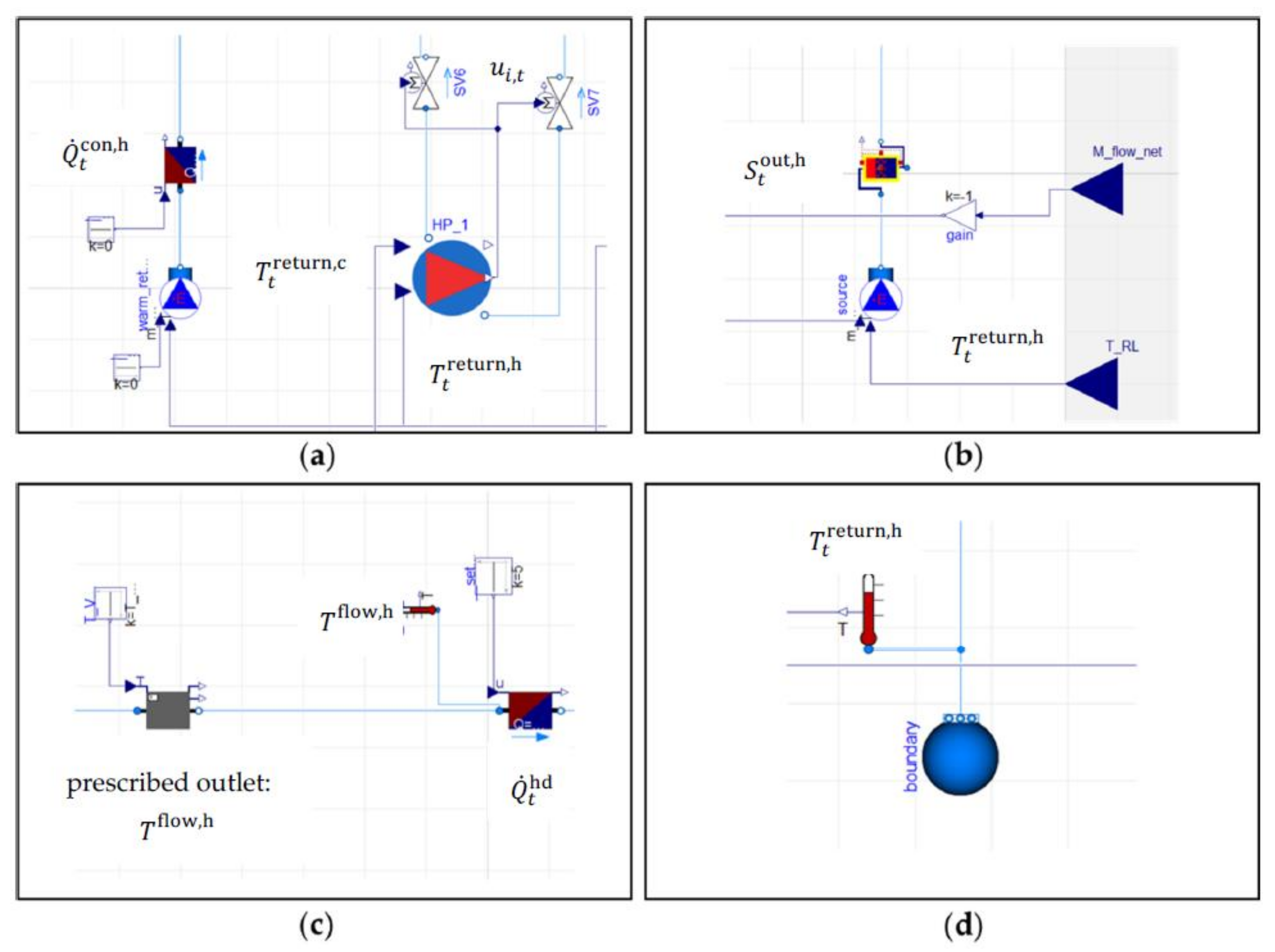
2.3. Simulation Model
A simulation model was developed for validation purposes (see
Figure 4).
The model was developed in the Modelica modeling language using the libraries: “ModelicaStandardLibrary” and “Buildings” [
25]. The generator circuit receives a signal with the current return temperature from the boundary block in
Figure 4d (“Modelica.Fluid.Sources.FixedBoundary”). The return strand is modeled by a source block (see
Figure 4b—“Modelica.Fluid.Sources.MassFlowSource_T”), which feeds into the generators with the corresponding return temperature. The respective mass flow rate is calculated for each generator based on the MILP results (
,
,
). The energy converter is modeled by a heating/cooling block (see
Figure 4a—“Buildings.Fluid.HeatExchangers.HeaterCooler_u”) and receives a signal
u of the current heat flow rate
. The heat pumps’ and storages’ inflow is controlled by a valve (SV6 or SV7 in
Figure 4a—“Modelica.Fluid.ValvesIncompressible”). The storage is modeled as stratified storage (see
Figure 4b—“Buildings.Fluid.Storage.Stratified”). The heat pumps (HP_1) cooling component is modeled by a heating/cooling block as well (“Buildings. Fluid.HeatExchangers.HeaterCooler_u”). It receives a signal of the current cold flow rate calculated by the COP and the electrical power, which are based on the regressor function from the MILP model and have the cold return temperature of every simulation step and the hot flow temperature as an input. A heating block (“Buildings. Fluid.HeatExchangers. Heater_T”) receives the electrical power, the COP, the maximum heat flow rate, and the needed heat flow temperature as inputs. The output of this block is the actual heat flow rate, which is needed to calculate the electrical power for the NPV
. Before the fluid flows into the consumer, its temperature is adjusted to the prescribed flow temperature
with the first block in
Figure 4c (“Buildings. Fluid.HeatExchangers.PrescribedOutlet”). The consumer is modeled with a heating/cooling block (“Buildings. Fluid.HeatExchangers.HeaterCooler_u”), and it receives the current demand
. Afterward, the fluid flows into the boundary block.
The results of the MILP model are necessary inputs for the simulation model. The simulation model requires information about the heat pump constellation () (heat pump model and purchase amount) and the storage size for the heating and cooling network, if needed. The operation signals of every energy converter in the generation circuit (including the storages) and the distribution circuit are passed to the simulation model as well. In conclusion, the following results and parameters are given to the simulation:
flow temperatures to adjust the heat pump operation,
regression function to calculate the and the maximum electrical power for the heat pump operation in the simulation with the simulation’s return temperature and the passed flow temperature ,
minimum electrical power to limit the heat pumps’ operation in the simulation,
time step to adjust the time series in the simulation,
buying decision to implement the heat pump constellation into the simulation,
storage volumes and to pass the dimension into the simulation,
heating and cooling demand at each time step to model the consumer in the simulation,
conventional heating and cooling at each time step to model a conventional energy converter in the simulation,
value of the objective function to insert it into Equation (17),
heat and cold flow rate of every heat pump at each time step to calculate the mass flow rates in the simulation,
loading and unloading heat flow rate for the storage to set it in the simulation.
The listing is summarized in
Table A4. The COP and the electrical power input of every heat pump are recalculated in each time step based on the resulting temperatures in the simulation (see regressor function in
Table A4). The heat and cold flow rates of the heat pumps in the simulation model are calculated in analogy with the mathematical model; however, the simulation has a much sharper resolution of 60 s time steps. In the simulation model, the fluid in front of the consumer is forced to emerge with the flow temperature
. In case of incorrect calculations in the mathematical optimization resulting in an incorrect flow temperature, the additional power to lift or lower the fluid’s temperature is added in terms of amount to the conventional energy converter
. After the simulation is finished, the new values for electrical power
and conventional heating/cooling
are inserted into Equation (1) to calculate the objective function value
for the simulation run. The error
between the objective values
and
is calculated using the following formula:


