Abstract
This paper proposes a coordinated voltage regulation method for active distribution networks (ADNs) to mitigate nodal voltage fluctuations caused by photovoltaic (PV) power fluctuations, where a three-stage optimization scheme is developed to coordinate and optimize the tap position of on-load tap changers (OLTCs), the reactive power of capacitor banks (CBs), and the active and reactive power of soft open points (SOPs). The first stage aims to schedule the OLTC and CBs hourly using the rolling optimization algorithm. In the second stage, a multi-objective optimization model of SOPs is established to periodically (15 min) optimize the active and reactive power of each SOP. Meanwhile, this model is also responsible for optimizing the Q-V droop control parameters of each SOP used in the third stage. The aim of the third stage is to suppress real-time (1 min) voltage fluctuations caused by rapid changes in PV power, where the Q-V droop control is developed to regulate the actual reactive power of SOPs automatically, according to the measured voltage at the SOPs’ connection points. Furthermore, numerous simulations and comparisons are carried out on a modified IEEE 33-bus distribution network to verify the effectiveness and correctness of the proposed voltage regulation method.
1. Introduction
In recent years, environment protection and sustainability have become the main concern across the whole world. As is known to all, the access of distributed generations (DGs), such as photovoltaic (PV) plants and wind turbines, can reduce environmental pollution and energy crisis, and the application of PV power systems is particularly important for the sustainable development of the environment. Recently, a large number of PV plants have been connected to low-voltage distribution networks [1,2,3], but their output power has strong uncertainty and randomness, resulting in significant nodal voltage variations [4,5,6]. With the increase of PV penetrations, the bus voltage of distribution networks may frequently violate the voltage constraints defined by utility grids, which will damage the voltage stability and power quality of active distribution networks (ADNs) [7]. Thus, studying the voltage regulation methods of ADNs is of great significance to the operating, scheduling, and planning of distribution networks.
Traditional voltage regulation measures include switching on/off capacitor banks (CBs) and changing the tap position of on-load tap changers (OLTCs) [8]. However, the disadvantages are that they not only need too much time to respond to the control commands, but also their lifetimes are limited [9], thus it is better to adjust their operating status as few times as possible. Clearly, using OLTCs and CBs is hard to fully solve the voltage issues of ADNs caused by active power fluctuations of high levels of PV. Therefore, to solve this problem, the active power of PV plants can be reduced to avoid bus voltages exceeding upper voltage constraints, but it will reduce the revenue of selling solar power [10,11]. Nowadays, using the rest capacity of PV converters to generate or absorb reactive power is a popular way for PV plants to participate in voltage regulation of ADNs [12,13]. However, it is difficult to centrally coordinate various PV plants due to their different ownership and the shortage of communication links between them. Furthermore, the usage of static var compensators, energy storage systems, and demand side response are also effective ways for regulating voltage variations [14,15,16]. However, unlike transmission systems, distribution networks have a large value of R/X, so that the voltage problem caused by power variations of large-scale PV plants cannot be effectively solved only by optimizing the reactive power distribution [17,18,19]. Therefore, the optimization of active and reactive power distribution of ADNs should be considered simultaneously to make full use of the advantages of various voltage control methods and devices, achieving a better voltage regulation result.
Recently, the technology of soft open points (SOPs) provides a new solution for voltage regulation of ADNs [20,21,22]. The SOP is a type of fully controlled power electronic devices, which can replace the tie switch in the traditional distribution network, and can significantly improve the flexibility and reliability of the system. Also, the greatest feature of the SOP is that the active and reactive power of its two sides can be controlled continuously and accurately. SOPs just need to ensure the active power balance, but they do not require that the reactive power outputs of two sides are the same [23,24,25]. For example, when one side of a SOP is absorbing reactive power, the other side can be controlled to generate or absorb reactive power.
Consequently, the active and reactive power profiles are optimized in [21] with the aim of minimizing total losses and bus voltage deviations of ADNs. Reference [24] mainly focuses on the coordination between SOPs and conventional tie switches, where the bus voltages can be mitigated within a certain range by the proposed bi-level model. References [26,27] allocate SOPs and DG units with or without network reconfiguration to optimize the voltage deviation index and load balancing index. In [28], a coordinated voltage and var control method based on SOPs and multiple regulation devices, such as the OLTC and CBs, is proposed, but all voltage control devices are optimized on the same time scale. As a result, this method has failed to fully utilize the fast voltage regulation capability of the SOPs. The above voltage regulation methods are centralized voltage control schemes, and the communication delays and a huge amount of calculations will significantly affect the voltage regulation results. In addition, the decentralized voltage control strategies based on SOPs can also be used to regulate the voltage variations in ADNs [29,30], but they neglect the uncertainties of renewable energy power outputs and loads during the optimization. The above methods can effectively control the voltage variations with a long-term timescale (≥15 min), but these methods have not fully discussed the schemes and strategies of mitigating the voltage variations under smaller timescales (e.g., 10 s, 1 min).
However, to the best of our knowledge, the methods of using SOPs to control voltage variations of ADNs have not been fully investigated, and further studies are required to improve the previous studies on the coordinated control schemes of SOPs and traditional voltage control devices. Hence, this paper aims to develop an optimal control method of SOPs, OLTCs, and CBs for limiting nodal voltage fluctuations of ADNs caused by PV power fluctuations, ensuring that the distribution network has smaller losses, and the OLTCs and CBs have longer lifetime. The main contributions of this study are the following:
(1) To minimize the bus voltage variations and operating losses of ADNs, a coordinated voltage control method for ADNs is developed, where the OLTC’s tap position, the reactive power of CBs, and the active and reactive power of SOPs are coordinated and optimized via a three-stage optimization scheme.
(2) Based on the rolling optimization algorithm, a mixed-integer nonlinear optimization model is established to hourly optimize the tap position of OLTC and the numbers of capacitors switched on each CB, where the uncertainties of PV outputs and load demands are fully considered.
(3) A multi-objective optimization model of SOPs aiming at reducing voltage variations and operating losses of ADNs is established to periodically optimize the short-term active power and reactive reference power of each SOP. A Q-V droop control algorithm for SOPs is developed to regulate the actual reactive power compensation of each SOP, according to the local bus voltage.
(4) Several simulations and comparisons are carried out on a modified IEEE 33-bus distribution system using the real data of PV plants to prove the effectiveness of the proposed voltage regulation method.
The rest of this paper is organized as follows: Section 2 describes the system structure of an ADN including SOPs. The proposed voltage regulation method is presented in Section 3, including the overall control scheme, objective functions, decision variables, constraints, and solution methods. Case studies and discussions are presented in Section 4, and the conclusions of this work are summarized in Section 5.
2. System Description
Figure 1 presents the system topology of an ADN, including an OLTC, SOPs, PV plants, and CBs. The SOP is a power electronic device, which is used to replace the traditional tie switch in distribution networks, and it can achieve precise power control between two feeders. Various structures of SOPs are presented in [23], including back to back voltage source converters (B2B VSC), the unified power flow controller (UPFC), and the static synchronous series compensator (SSSC). This paper takes the B2B VSC as an example to investigate the coordinated voltage regulation methods of ADNs. The B2B VSC consists of two VSC converters, i.e., SOP-ij shown in Figure 1. Also, the SOP has stronger power regulation ability and faster response speed compared with conventional voltage regulation devices. Different from the mechanical voltage regulation devices such as OLTCs, the SOP is a fully controlled power electronic converter and can quite quickly regulate its outputs of two sides [23,24,31]. In addition, the SOP can play a critical role in fault isolation and power restoration, because the fault current can be limited by the converters on both sides of the SOP, due to the isolation of the DC link [25].
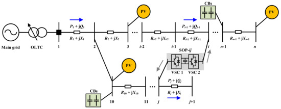
Figure 1.
System topology of an active distribution network (ADN) including the soft open point (SOP).
In this study, the total number of buses, branches, and CBs in the ADN are N, L, and H, respectively. i and j are the index of buses (nodes), i, j ∈ Φnode = {1,2,…, N}. l is the index of branches, l ∈ Φbran = {1,2,…, L}. Rl + jXl is the impedance of branch l, and Vi denotes the voltage of bus i. The set Vnode consists of the voltage of all buses, Vi ∈ Vnode. Ibran is a set of the current of all branches, Ibran = {I1, I2,…, Il}. So denotes the tap position of the OLTC, and Sc,i is the number of capacitors that are switched on CB i. The set SC = {Sc,1, Sc,2,…, Sc,H}. The active and reactive power of the i side (j side) of SOP-ij are denoted by and ( and ), respectively. The sets PS and QS consist of active and reactive power of all SOPs, i.e., , ∈ PS, and , ∈ QS. The demand at bus i is + jQload,i, and the active power injection of PV at bus i is , whereas the reactive power output of CB i is denoted by . Also, t denotes the current time.
As can be seen from Figure 1, the output power fluctuations of a PV plant not only lead to voltage violations where the PV plant is connected to but also affect the voltage of other buses at the same feeder. When numerous PV plants installed in this ADN, the power quality will be extremely terrible if without any effective control ways. For example, sometimes, the bus voltage exceeds the upper voltage limit if the PV power is larger than loads, and sometimes the voltage may suddenly drop due to the rapid decline in PV power. Therefore, this study develops a voltage control method to avoid the above-discussed voltage issues.
3. Coordinated Voltage Regulation Methods
This section first gives the overall idea of the proposed voltage regulation methods, discusses the objective functions and decision variables of each stage, and explains the coordination relationships between each control stage. Then, the specific mathematical models and solution methods of this voltage control method are described, respectively.
3.1. Overall Idea of the Proposed Voltage Regulation Methods
In this study, a coordinated control method of the OLTC, CBs, and SOPs is proposed to limit the nodal voltage variations of ADNs, which is achieved by optimizing the OLTC tap position, the reactive power compensation of CBs, and the active and reactive power output of SOPs. Therefore, the optimization described above is divided into three stages, as shown in Figure 2.
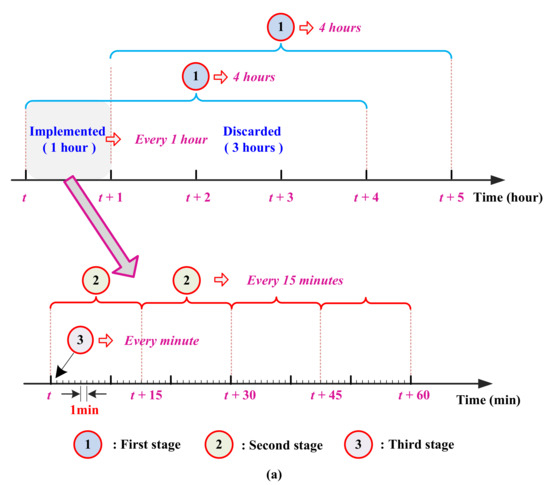
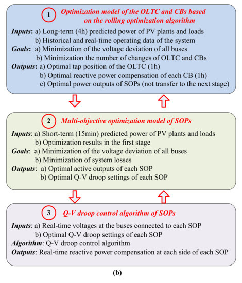
Figure 2.
Overall ideas of the proposed voltage regulation method: (a) The timescale of each stage; (b) input parameters, objective functions, and decision variables of each stage.
3.1.1. First Stage (Long-Term Optimization)
In the first stage, an optimization model of the OLTC and CBs is established based on the rolling optimization algorithm, which mainly focuses on optimizing the tap position of the OLTC and the reactive power output of each CB. Thus, the long-term bus voltage variations caused by periodical changes of PV outputs and loads can be reduced. To reduce the number of changes of OLTCs and CBs, the optimization is implemented every 1 h according to the long-term predicted power of PV plants and loads.
In summary, the objective function of the first stage is to minimize the voltage deviations and the number of changes of the OLTC and CBs. The decision variables consist of the OLTC tap position (So), the number of capacitors switched on each CB (Sc,i), and the active and reactive power of each SOP (, , , and ). In this stage, SOPs are involved in the optimization process, but the optimization results of SOPs are not sent to the next stage. The actual outputs of SOPs are determined by the control method proposed in the second stage and third stage.
3.1.2. Second Stage (Short-Term Optimization)
The first stage determines the operating status of the OLTC and CBs in the next 1 h, hence the second stage aims to regularly optimize the running condition of all SOPs during the next 15 min. Therefore, a multi-objective optimization model of SOPs is established, and the model is executed every 15 min to achieve the following two goals:
(1) To optimize the active power injection by each SOP.
(2) To optimize the Q-V droop coefficients at each side of all SOPs. The Q-V droop control used in the third stage is to dynamically adjust the reactive power of SOPs, according to the real-time local bus voltage and the droop settings.
In summary, the objective function of the second stage is to minimize total bus voltage deviations and system losses, while the decision variables of the second stage are active power of SOPs ( and ), reference reactive power of SOPs ( and ), and the Q-V droop settings of SOPs. Eventually, the optimization results will be sent to the third stage.
3.1.3. Third Stage (Real-Time Control)
The third stage is executed every minute to mitigate the real-time nodal voltage variations. The Q-V droop control strategy is used for all SOPs to control the real-time reactive outputs in both sides of them. Namely, a SOP will automatically adjust its reactive power compensation based on the updated Q-V droop settings and the sampled voltage at the bus connected to the SOP.
In addition to the final reactive power outputs of SOPs, the remaining control variables just follow the control commands generated in the above two stages.
As explained above, the proposed voltage control method can make sure that the nodal voltage variations can be reduced as much as possible, through the coordination between these three stages. Their specific mathematical models are described in the following sections.
3.2. Optimization Models of the OLTC and CBs
This section discusses how to use the rolling optimization algorithm to determine the tap position of an OLTC and the reactive outputs of CBs. Hence, this section begins by describing the rolling optimization framework and goes on to discuss mathematical expressions of the established models.
3.2.1. Rolling Optimization Framework
In order to account for the uncertainties of PV outputs and loads, a rolling optimization is developed, which is shown in Figure 3 [32,33]. First, some advanced prediction techniques are utilized to predict the output power of all PV plants and the load power from time t1 to t1 + ΔT1, where ΔT1 is the total prediction time, e.g., 4 h in this study, and the predicted time interval Δt1 is 1 h in this study. Then, taking the predicted data and the current operation data of ADNs as the input, the objective function will be minimized to gain the optimal profiles of the OLTC’s tap position and the reactive outputs of CBs from time t1 to t1 + ΔT1. However, only the optimization results of the first hour (i.e., from time t1 to t1 + Δt1) are adopted, and the remaining optimization results (i.e., from time t1 + Δt1 to t1 + ΔT 1) are neglected.
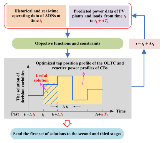
Figure 3.
Principle of optimizing the on-load tap changer’s (OLTCs) tap position and capacitor banks’ (CBs’) reactive outputs using the rolling optimization algorithm.
Finally, the above optimization will be executed again at t1 + Δt1, and the predicted data of PV plants and loads will be updated. Hence, we can get more accurate and effective optimization results, compared with the cases where all optimal solutions were adopted.
3.2.2. Mathematical Models
The objective function of the established optimization model, f1, aims at minimizing the total voltage deviations of all nodes and the number of changes of OLTC and CBs, as follows:
Objective function:
where So, SC, PS, and QS are decision variables. Function Udev denotes the voltage variation of all nodes in the ADN, and functions FCB and FOLTC denote the changing times of the OLTC and CBs during the current optimization period, respectively. ρ1 and ρ2 are weight coefficients and are utilized to represent the importance of the sub-objective functions, and ρ1 + ρ2 = 1. The larger value of ρ1 is, the more important the sub-objective function Udev is. Since the minimization of nodal voltage variations is the primary concern of voltage regulation for ADNs, the sub-objective function Udev is more important than functions FCB and FOLTC in the objective function f1. The analytic hierarchy process(AHP) [28] has been wildly used in complex decision-making problems, which can determine the weight coefficients of sub-objective functions in terms of the importance of them. Therefore, this paper uses the AHP to determine the values of ρ1 and ρ2, and this paper sets ρ1 = 0.87, ρ2 = 0.13. VL and VU are ideal voltage variation limits, e.g., VL = 0.98 p.u. and VU = 1.02 p.u [29].
Constraints:
The model should meet the power flow constraints, as follows. (5)–(10) are power flow constraints, where (5) and (6) are active and reactive power balance equations; (11) is the bus voltage limit, and (12) denotes the branch current limit. (13)–(18) are the operating requirements of the OLTC and CBs, respectively. Moreover, the constraints of SOPs are described by (19)–(23), where the active power balance of a SOP is described in (19)–(21), and the reactive power limit at each side of a SOP is described in (22). Also, (23) requires that the total active and reactive output at each side of a SOP should be less than its capacity.
where Pij and Qij are active and reactive power flows of branch ij; Pi and Qi are active and reactive power injections at bus i, respectively; Rij and Xij are resistance and reactance of branch ij, respectively. V1 is the voltage of bus 1, and ΔUo is the voltage step of the OLTC. ΔQc,i is the unit capacity of a capacitor in CB i. It is assumed that the statutory voltage range is [Vmin, Vmax], e.g., [0.95, 1.05] p.u. [28]. Il,max is the maximum allowable current of branch l. The range of is [, ], and the range of is [0, ]. γo,max and γc,max denote the maximum allowed adjustments of an OLTC and a CB during the current optimization period, respectively. Furthermore, (), (), and () denote the active power, reactive power and the active power loss at the i side (j side) of the SOP-ij, respectively. is the rated capacity of SOP-ij, and μ is the loss coefficient of SOPs, i.e., a factor for evaluating the active power loss of SOPs [29,30,31].
3.3. Optimization Models of SOPs
In this section, as shown in Figure 4, the established multi-objective optimization model of SOPs will be executed twice using the known tap position of the OLTC, reactive outputs of all CBs, and the predicted power of all PV plants and loads during the period from time t to t + ΔT2 (ΔT2 = 15 min in this study).
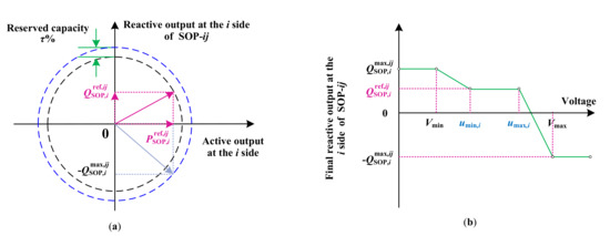
Figure 4.
Methods of optimizing the output power of SOPs: (a) Schematic diagram of optimizing the active and basic reactive power at the i side of SOP-ij; (b) schematic diagram of optimizing the Q-V droop coefficients at the i side of SOP-ij.
(1) For the first time of executing this model, the active and basic reactive outputs of each SOP during the period from time t to t + ΔT2 are determined, e.g., decision variables are and for SOP-ij at the i side, as shown in Figure 4a. However, will be directly sent to the SOP-ij as a control command, while will be regarded as the basic reactive power compensation at the i side of the SOP-ij, as shown in Figure 4b. The final reactive outputs of SOPs will be determined by the droop control in the third stage. Furthermore, the capacities of SOPs are reserved τ% during this optimization, as shown in Figure 4a, and the reserved capacity will be used when optimizing the Q-V droop coefficients of each SOP.
(2) For the second time of executing this model, and (i, j Φnode) are the known quantities. Thus, the decision variables are Q-V droop coefficients for each SOP, e.g., umin,i and umax,i shown in Figure 4b. Note that is related to the reserved capacity and the optimization results in the first optimization.
Therefore, the following section describes the mathematical expressions of the established multi-objective optimization model of SOPs in two steps.
3.3.1. Optimization of Active and Reactive Power of SOPs
The objective function of the established multi-objective optimization model, f2, aims at minimizing the total voltage deviations of all nodes, Udev, and the total operating losses of entire ADNs and all SOPs, Ploss, as follows:
where Ploss is the active power loss of ADN and SOPs. ρ3 and ρ4 are weight coefficients. As explained in earlier, this paper utilizes the AHP to decide the values of ρ3 and ρ4. Considering that the voltage has been controlled to a certain extent in the previous stage, this stage mainly focuses on the minimization of power losses of the system. Therefore, this paper sets ρ3 = 0.3, ρ4 = 0.7.
In the first step, the decision variables are , , , and , i, j Φnode and i ≠ j. Also, the constraints (5)–(12), and (19)–(23) are described in Section 3.2.2, where the variables and should be replaced with and , respectively; the loads and PV power at time t can be predicted using a short-term power prediction method. In addition to these constraints, the following constraint indicates the reserved SOP capacity:
3.3.2. Optimization of Q-V Droop Coefficients of SOPs
In the second step, the objective function is optimized again based on the same power data of PV plants and loads as well as the optimization results obtained in the first step, but decision variables and some constraints are changed. Namely, decision variables are Q-V droop coefficients at the i and j sides of the SOP-ij, i.e., umin,i(t), umax,i(t), umin,j(t), and umax,j(t), i, j Φnode and i ≠ j, as shown in Figure 4b. In addition to the constraints described in (5)–(12) and (19)–(22), the following constraints are added:
where and are the maximum allowed reactive power compensation at each side of SOP-ij; functions gi and gj can respectively find the reactive power compensation of SOP-ij corresponding to the bus voltage Vi and Vj on the Q-V droop curves. Taking gi(Vi(t)) as an example, it can be calculated as follows:
3.4. Q-V Droop Control of SOPs
As shown in Figure 5, at time t, each SOP automatically adjusts its reactive outputs at both sides according to the real-time bus voltages and the updated Q-V droop curves. For example, for the droop curve at the i side of SOP-ij, if the real-time voltage at bus i is within a range of [umin,i, umax,i], the final reactive output at the i side is equal to , which is determined in Section 3.3.1, otherwise, the final value of is determined by the droop curve.
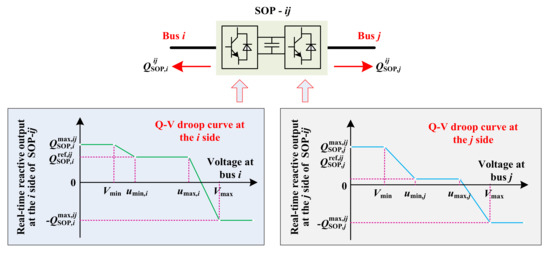
Figure 5.
The Q-V droop control of a SOP.
3.5. Solution Algorithms of All Established Models
This section discusses the methods of solving the established optimization models. It can be seen that the model in the first stage is a mixed-integer nonlinear programming (MINLP) problem, and the model developed in the second stage is a nonlinear programming (NLP) problem. Meanwhile, they all contain quadratic constraints. To solve this problem, the original models are transformed into the mixed integer second-order cone programming (MISOCP) problem by conic relaxations.
3.5.1. Conversion to an MISOCP Model
Therefore, this study converts these models into MISOCP model, where the objective functions and nonlinear constraints will be linearized. The MISOCP has been widely used in the planning and operation optimization of distribution networks, because it can quickly and effectively solve nonlinear programming problems [28,29,30,31]. In this work, constraints that need to be converted are:
- (1)
- Power flow constraints: (5)–(12).
- (2)
- Operation constraints of OLTCs and CBs: (13)–(18).
- (3)
- SOP constraints: (19)–(23) and (26)–(27).
- (4)
- Constraints related to droop control of SOPs: (28)–(30).
Among the constraints listed above, in addition to the constraints (28)–(30), the conversion methods of the remaining constraints have been fully demonstrated and used. Thus, this study will not discuss them carefully, and their details can be found in [28]. Linearization of constraints (28)–(30) is performed by introducing auxiliary variables, as follows:
where λi,k (k = 1,2,…,6) is used to accurately describe the position corresponding to the current voltage on the droop curve, and the nonlinear part umin,i(t)λi,3(t) is linearized using auxiliary variables xi,d, βi,d, ηi,d, and M, as shown in (33)–(36). xi,d and ηi,d are binary variables (i.e., 0–1 variables), and M is a large positive integer. Also, umax,i(t)λi,4(t) can be linearized using the same method.
In addition, to ensure that the reactive power compensation corresponding to the current voltage on the droop curve is unique, the following equations should be added:
where (k = 1,2,…,6) are binary variables, representing five line segments in the droop curve, respectively, and they are adopted to limit the range of (k = 1,2,…,6).
3.5.2. Calculation
In this work, the MISOCP models are solved on the MATLAB@R2015b platform (2015 release, The MathWorks, Inc., Natick, MA, USA), where the decision variables, objective functions, and constraints are described using the YAMLIP toolbox (R20190425, Johan Löfberg, Linköping University, Sweden), and the commercial solver IBM ILOG CPLEX (version 12.6, IBM Corporation, Armonk, NY, USA) [31] is utilized to find the best solution of the established optimization models. In addition, all the simulations are conducted on a PC with Windows10 OS, Inter(R) Core i7 CPU @1.80 GHz, and 8.0 GB RAM.
4. Case Study
4.1. Simulation Parameters
In this work, the proposed voltage regulation method is verified on a modified IEEE 33-bus radial distribution system, as shown in Figure 6. An OLTC is connected to bus 1, and its voltage regulation range is [0.95, 1.05] p.u. (0.005 p.u./step). CBs 1 and 2 are installed at buses 18 and 22, respectively. The total capacity of each CB is 300 kVar, including 5 capacitors. SOP 1 and SOP 2 are connected to buses 18 and 33, as well as buses 25 and 29, respectively. The capacity of each SOP is 800 kVA, and the loss coefficient is 0.02 [31]. The installed capacity and location of each PV plant is shown in Table 1. In addition, the daily power profiles of each PV plant are obtained from a real 750 kWp PV plant located in Sri Lanka [10], and the load power profile is obtained from [28], which is a typical daily power curve for industrial loads, as shown in Figure 7.
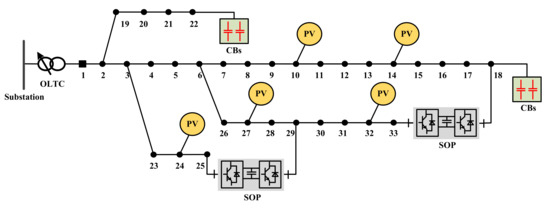
Figure 6.
A modified IEEE 33-node system with an OLTC, photovoltaic (PV) plants, CBs and SOPs.

Table 1.
Installed capacities and locations of PV plants.
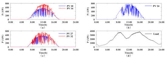
Figure 7.
Daily power profiles of each PV plant and all loads: (a) PV plants connected to feeder1; (b) PV plants connected to feeder2; (c) PV plants connected to feeder3; (d) all loads.
4.2. Simulation Results
4.2.1. Voltage Regulation Results
Based on the simulation cases described above, the voltage profiles after performing the proposed voltage regulation method are presented in Figure 8, and the voltage profiles without performing any voltage control scheme are shown in Figure 9.
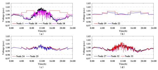
Figure 8.
Daily voltage profiles after performing the proposed voltage regulation method: (a) Feeder1; (b) Feeder2; (c) Feeder 3; (d) Feeder 4.
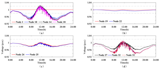
Figure 9.
Daily voltage profiles before performing the proposed voltage regulation method: (a) Feeder1; (b) Feeder2; (c) Feeder 3; (d) Feeder 4.
Looking at Figure 8, the bus voltage fluctuations are within the ideal range, [0.9800, 1.0195], whereas the original voltage fluctuation range is [0.9352, 1.0260] (without optimization) in Figure 9, and the average bus voltage deviation is reduced from 1.7854 p.u. to 1.1588 p.u. They indicate that the proposed voltage control scheme can effectively mitigate bus voltage fluctuations caused by PV power variations. Furthermore, the total system loss is reduced from 1113.65 kWh to 594.98 kWh after optimization, indicating that the proposed voltage control method has a remarkable effect on reducing operating losses of distribution networks.
4.2.2. Optimization Results of the OLTC and CBs
After optimization, the optimal tap position of the OLTC and the reactive outputs of each SOP are shown in Figure 10, where the OLTC is adjusted 8 times a day, and the number of daily adjustments of all CBs is 10 times. Furthermore, when the PV power generation is at a high level, the voltage at bus 1 is reduced by declining the OLTC’s tap position. Meanwhile, the CBs correspondingly reduce their reactive outputs to avoid the bus voltage exceeding the upper voltage limit. These results show that the developed optimization model of the OLTC and CBs based on the rolling optimization algorithm can correctly regulate their operation status and reduce their changing times.
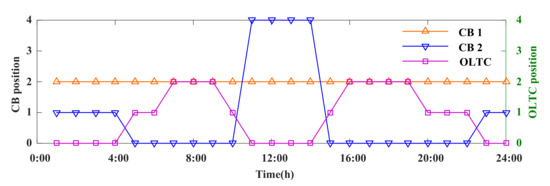
Figure 10.
Optimal profile of the tap position of the OLTC and CBs.
4.2.3. Optimal Active and Reactive Power Profiles of SOPs
After optimization, the real-time active and reactive outputs at each side of SOP are shown in Figure 11.
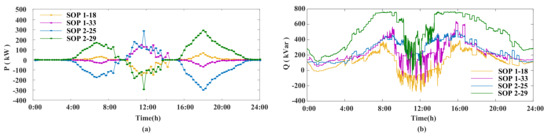
Figure 11.
Daily power profiles of each SOP after optimization: (a) Active power; (b) reactive power.
As can be seen from Figure 11b, for any SOP, their reactive outputs of both sides are independent and can be regulated flexibly and separately. In summary, these results indicate that the established multi-objective optimization model of SOPs can properly allocate and coordinate the active outputs and reactive power compensation of all SOPs, ensuring that they can effectively respond to various bus voltage fluctuations.
As discussed earlier, the Q-V droop coefficients of each SOP are optimized after optimizing the active and reactive power of SOPs. Therefore, in order to further explain the relationship between the basic reactive power compensation and the final reactive outputs of SOPs, the following simulations discuss the reactive power regulation process of the SOP connected at bus 18 and 33. Figure 12 shows the optimized Q-V droop coefficients, initial bus voltages, and final reactive outputs of the SOP 18–33 from 11:00 to 12:00.
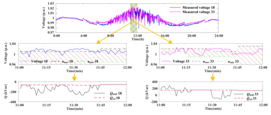
Figure 12.
Optimized Q-V droop coefficients, initial bus voltages, and final reactive outputs of the SOP 18–33 from 11:00 to 12:00.
As can be seen from Figure 12, during 11:01–11:30, the dead zone of Q-V droop curve at bus 18 is [0.96, 1.01] p.u., and the basic reactive power compensation of the SOP is −65 kVar. Hence, the final reactive power output is equal to −65 kVar if the real-time voltage at bus 18 is within the dead zone, [0.96, 1.01]. However, sometimes the voltage at bus 18 exceeds the upper limit of the dead zone, thus the SOP correspondingly reduces its reactive output. Similarly, the SOP increases its reactive power output if the voltage at bus 33 is lower than the lower limit of the dead zone from 11:01 to 11:15. These results demonstrate that the proposed Q-V droop control strategy of SOPs can effectively regulate the reactive power compensation of each SOP to reduce the real-time bus voltage fluctuations.
4.3. Comparisons of Different Voltage Regulation Methods
To analyze the advantages and disadvantages of the proposed voltage control methods, five methods are compared and analyzed under the same case. The reference voltage control methods are summarized as follows:
Method I: No voltage control scheme is conducted on ADNs, i.e., ADNs are operating without performing any voltage control scheme.
Method II: A combined voltage control method is proposed in [30], where only SOPs are utilized to regulate the voltage variations of ADNs.
Method III: This method is the combination of the method developed in [30] and the control scheme used in the first stage of the proposed voltage control.
Method IV: This method does not consider the optimization of Q-V droop settings of SOPs, and the remaining control process is the same as the method developed in this paper. Also, the Q-V droop settings of SOPs are set to the values used in [13].
Method V: The proposed voltage control method is conducted without the Q-V droop control of SOPs. Namely, the reactive power output of SOPs in the third stage is the fixed value after performing the second stage optimization.
Table 2 shows the optimization results of different voltage regulation methods. In addition, the minimum and maximum voltage distribution of the ADN is shown in Figure 13.
Table 2.
Comparisons of different voltage regulation methods.
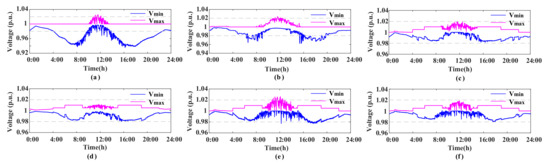
Figure 13.
The minimum and maximum voltage based on different control methods: (a) Method I; (b) Method II; (c) Method III; (d) Method IV; (e) Method V; (f) Proposed method.
Looking at Table 2 and Figure 13, compared with method I, the average voltage deviation of method II reduces from 1.7854 p.u. to 1.3219 p.u., and the overall operating losses of method II reduces from 1113.65 kWh to 799.94 kWh, which shows that the use of SOPs is effective in reducing voltage variations and operating losses of ADNs.
After adding the first stage optimization model of the proposed voltage control method into method II, method III results in lower operating losses and lower average voltage deviation compared to method II. In addition, the voltage variations after control are in the ideal range. These results indicate that the established optimization model of the OLTC and CBs can effectively deal with the uncertainties of the PV outputs and loads. Compared with method III, the active and reactive power are optimized cooperatively in the second stage of the proposed method, and SOPs still have reactive power outputs in the dead zone. Therefore, the operating losses can be significantly reduced.
Both method IV and the proposed voltage control method can control the voltage variations of all nodes within the required voltage range, but the average operating losses of method IV are significantly larger than those of the proposed method. It indicates that optimizing Q-V droop settings according to the PV outputs and network structure and making full use of SOPs’ regulation abilities are helpful in reducing the operating losses of ADNs.
For method V, the output power of SOPs is optimized every 15 min, thus it cannot effectively mitigate the voltage changes during the control interval. Although method V and the proposed method have almost the same performance in reducing operating losses, the average voltage deviations of method V are larger than those of the method developed in this work. These results show that the real-time Q-V droop control of SOPs plays an important role in regulating real-time voltage fluctuations caused by rapid changes in PV power.
In conclusion, the above comparisons show that the proposed voltage control method can make full use of the voltage regulation capability of SOPs, and the operating losses and voltage fluctuations of ADNs can be remarkably minimized.
5. Conclusions
The main goal of the current study was to find a new method to regulate voltage variations using SOPs in ADNs considering uncertainties. A coordinated three-stage voltage regulation method for ADNs is proposed to mitigate nodal voltage fluctuations caused by PV power fluctuations, where the active and reactive power of SOPs, the OLTC tap position, and the reactive power compensation of CBs are optimized in the distribution network level. The main findings are summarized as follows:
(1) The proposed voltage regulation method can not only reduce voltage deviations of all nodes in ADNs, but also can reduce the operating losses.
(2) For a SOP with a certain capacity, the optimization of its active and reactive output power should be considered at the same time, ensuring that the SOP can be fully used to participate in the voltage regulation of ADNs.
(3) When utilizing Q-V droop control algorithm to regulate real-time reactive power of SOPs according to the measured voltage at their connection points, a better voltage regulation result can be obtained if the Q-V droop settings are dynamically optimized in terms of the predicted power of PV plants and loads as well as the topology of ADNs.
(4) In this study, the reactive power corresponding to the dead zone of the Q-V droop curve is periodically optimized, instead of setting the reactive power to zero. Such optimization can not only increase the capability of SOPs in regulating voltage fluctuations, but also can decrease the operating losses of ADNs.
The current study has not been able to consider the coordination between PV plants and SOPs, because this paper mainly aims to investigate the capability of SOPs in controlling voltage variations. Therefore, more researches are required to examine coordinated control methods for SOPs, PV plants, OLTCs, and CBs to suppress nodal voltage fluctuations in ADNs.
Author Contributions
Writing—original draft, R.H.; writing—review and editing, W.W., Z.C., X.W. and W.M.; data curation, X.W. and L.J.; supervision, G.Z. All authors have read and agreed to the published version of the manuscript.
Funding
This research was funded by the China Southern Power Grid Co., Ltd. Science and Technology Project grant number [090000KK52180116].
Conflicts of Interest
The authors declare no conflict of interest.
References
- Sarkar, M.N.I.; Meegahapola, L.G.; Datta, M. Reactive power management in renewable rich power grids: A review of grid-codes, renewable generators, support devices, control strategies and optimization algorithms. IEEE Access 2018, 6, 41458–41489. [Google Scholar] [CrossRef]
- Ma, C.; Dong, S.; Lian, J.; Pang, X. Multi-objective sizing of hybrid energy storage system for large-scale photovoltaic power generation system. Sustainability 2019, 11, 5441. [Google Scholar] [CrossRef]
- Wang, H.; Wang, J.; Piao, Z.; Meng, X.; Sun, C.; Yuan, G.; Zhu, S. The optimal allocation and operation of an energy storage system with high penetration grid-connected photovoltaic systems. Sustainability 2020, 12, 6154. [Google Scholar] [CrossRef]
- Aziz, T.; Ketjoy, N. Enhancing PV penetration in LV networks using reactive power control and on load tap changer with existing transformers. IEEE Access 2018, 6, 2683–2691. [Google Scholar] [CrossRef]
- Kacejko, P.; Adamek, S.; Wydra, M. Optimal voltage control in distribution networks with dispersed generation. In Proceedings of the 2010 IEEE PES Innovative Smart Grid Technologies Conference Europe (ISGT Europe), Gothenberg, Sweden, 11–13 October 2010; pp. 1–4. [Google Scholar]
- Krata, J.; Saha, T.K.; Yan, R. Model-driven real-time control coordination for distribution grids with medium-scale photovoltaic generation. IET Renew. Power Gener. 2017, 11, 1603–1612. [Google Scholar] [CrossRef]
- Wang, L.; Yan, R.; Saha, T.K. Voltage management for large scale PV integration into weak distribution systems. IEEE Trans. Smart Grid 2018, 9, 4128–4139. [Google Scholar] [CrossRef]
- Zhang, C.; Xu, Y.; Dong, Z.; Ravishankar, J. Three-stage robust inverter-based voltage/var control for distribution networks with high-level PV. IEEE Trans. Smart Grid 2019, 10, 782–793. [Google Scholar] [CrossRef]
- Xu, Y.; Dong, Z.Y.; Zhang, R.; Hill, D.J. Multi-timescale coordinated voltage/var control of high renewable-penetrated distribution systems. IEEE Trans. Power Syst. 2017, 32, 4398–4408. [Google Scholar] [CrossRef]
- Ma, W.; Wang, W.; Wu, X.; Hu, R.; Tang, F.; Zhang, W.; Han, X.; Ding, L. Optimal allocation of hybrid energy storage systems for smoothing photovoltaic power fluctuations considering the active power curtailment of photovoltaic. IEEE Access 2019, 7, 74787–74799. [Google Scholar] [CrossRef]
- Aziz, T.; Ketjoy, N. PV penetration limits in low voltage networks and voltage variations. IEEE Access 2017, 5, 16784–16792. [Google Scholar] [CrossRef]
- Liu, X.; Cramer, A.M.; Liao, Y. Reactive power control methods for photovoltaic inverters to mitigate short-term voltage magnitude fluctuations. Electr. Power Syst. Res. 2015, 127, 213–220. [Google Scholar] [CrossRef]
- Turitsyn, K.; Sulc, P.; Backhaus, S.; Chertkov, M. Options for control of reactive power by distributed photovoltaic generators. Proc. IEEE 2011, 99, 1063–1073. [Google Scholar] [CrossRef]
- Zakariazadeh, A.; Homaee, O.; Jadid, S.; Siano, P. A new approach for real time voltage control using demand response in an automated distribution system. Appl. Energy 2014, 117, 157–166. [Google Scholar] [CrossRef]
- Ma, W.; Wang, W.; Wu, X.; Hu, R.; Tang, F.; Zhang, W. Control strategy of a hybrid energy storage system to smooth photovoltaic power fluctuations considering photovoltaic output power curtailment. Sustainability 2019, 11, 1324. [Google Scholar] [CrossRef]
- Fang, L.; Luo, A.; Xu, X.; Fang, H.; Ma, F.; Wang, W. Voltage control for static var compensator using novel optimal nonlinear PI. J. Control Theory Appl. 2012, 10, 35–43. [Google Scholar] [CrossRef]
- Collins, L.; Ward, J.K. Real and reactive power control of distributed PV inverters for overvoltage prevention and increased renewable generation hosting capacity. Renew. Energy 2015, 81, 464–471. [Google Scholar] [CrossRef]
- Ghasemi, M.A.; Parniani, M. Prevention of distribution network overvoltage by adaptive droop-based active and reactive power control of PV systems. Electr. Power Syst. Res. 2016, 133, 313–327. [Google Scholar] [CrossRef]
- Wang, J.; Bharati, G.R.; Paudyal, S.; Ceylan, O.; Bhattarai, B.P.; Myers, K.S. Coordinated electric vehicle charging with reactive power support to distribution grids. IEEE Trans. Ind. Inform. 2019, 15, 54–63. [Google Scholar] [CrossRef]
- Shafik, M.B.; Chen, H.; Rashed, G.I.; El-Sehiemy, R.A.; Elkadeem, M.R.; Wang, S. Adequate topology for efficient energy resources utilization of active distribution networks equipped with soft open points. IEEE Access 2019, 7, 99003–99016. [Google Scholar] [CrossRef]
- Long, C.; Wu, J.; Thomas, L.; Jenkins, N. Optimal operation of soft open points in medium voltage electrical distribution networks with distributed generation. Appl. Energy 2016, 184, 427–437. [Google Scholar] [CrossRef]
- Cao, W.; Wu, J.; Jenkins, N.; Wang, C.; Green, T. Benefits analysis of soft open points for electrical distribution network operation. Appl. Energy 2016, 165, 36–47. [Google Scholar] [CrossRef]
- Bloemink, J.M.; Green, T.C. Benefits of Distribution-Level Power Electronics for Supporting Distributed Generation Growth. IEEE Trans. Power Deliv. 2013, 28, 911–919. [Google Scholar] [CrossRef]
- Gu, H.; Chu, X.; Tang, M. Coordinated control of tie switch and soft normally open point for harnessing flexibility in active distribution systems. J. Phys. Conf. Ser. 2019, 1176, 62052. [Google Scholar] [CrossRef]
- Aithal, A.; Li, G.; Wu, J.; Yu, J. Performance of an electrical distribution network with soft open point during a grid side AC fault. Appl. Energy 2018, 227, 262–272. [Google Scholar] [CrossRef]
- Diaaeldin, I.; Abdel Aleem, S.; El-Rafei, A.; Abdelaziz, A.; Zobaa, A.F. Optimal network reconfiguration in active distribution networks with soft open points and distributed generation. Energies 2019, 12, 4172. [Google Scholar] [CrossRef]
- Zheng, Y.; Song, Y.; Hill, D.J. A general coordinated voltage regulation method in distribution networks with soft open points. Int J. Electr. Power 2020, 116, 105571. [Google Scholar] [CrossRef]
- Li, P.; Ji, H.; Wang, C.; Zhao, J.; Song, G.; Ding, F.; Wu, J. Coordinated control method of voltage and reactive power for active distribution networks based on soft open point. IEEE Trans. Sustain. Energy 2017, 8, 1430–1442. [Google Scholar] [CrossRef]
- Li, P.; Ji, H.; Yu, H.; Zhao, J.; Wang, C.; Song, G.; Wu, J. Combined decentralized and local voltage control strategy of soft open points in active distribution networks. Appl. Energy 2019, 241, 613–624. [Google Scholar] [CrossRef]
- Zhao, J.; Yao, M.; Yu, H.; Song, G.; Ji, H.; Li, P. Decentralized voltage control strategy of soft open points in active distribution networks based on sensitivity analysis. Electronics 2020, 9, 295. [Google Scholar] [CrossRef]
- Ji, H.; Wang, C.; Li, P.; Ding, F.; Wu, J. Robust operation of soft open points in active distribution networks with high penetration of photovoltaic integration. IEEE Trans. Sustain. Energy 2019, 10, 280–289. [Google Scholar] [CrossRef]
- O’Connell, A.; Flynn, D.; Keane, A. Rolling multi-period optimization to control electric vehicle charging in distribution networks. IEEE Trans. Power Syst. 2014, 29, 340–348. [Google Scholar] [CrossRef]
- Dhulipala, S.C.; Monteiro, R.V.A.; Silva Teixeira, R.F.D.; Ruben, C.; Bretas, A.S.; Guimaraes, G.C. Distributed model-predictive control strategy for distribution network volt/var control: A smart-building-based approach. IEEE Trans. Ind. Appl. 2019, 55, 7041–7051. [Google Scholar] [CrossRef]


Publisher’s Note: MDPI stays neutral with regard to jurisdictional claims in published maps and institutional affiliations. |
© 2020 by the authors. Licensee MDPI, Basel, Switzerland. This article is an open access article distributed under the terms and conditions of the Creative Commons Attribution (CC BY) license (http://creativecommons.org/licenses/by/4.0/).