Article

The Risk Monitoring of the Financial Ecological Environment in Chinese Outward Foreign Direct Investment Based on a Complex Network

1
School of Management, Wuhan University of Technology, Wuhan 430070, China
2
Alliance Manchester Business School, The University of Manchester, Manchester M15 6PB, UK
*
Author to whom correspondence should be addressed.
Sustainability 2020, 12(22), 9456; https://doi.org/10.3390/su12229456
Submission received: 19 October 2020 / Revised: 6 November 2020 / Accepted: 11 November 2020 / Published: 13 November 2020

Abstract

:
Aiming at the risk problem of financial ecological environment in outward foreign direct investment (OFDI), this paper constructs a risk monitoring model of the financial ecological environment based on complex network theory, and analyzes the general laws of financial risk evolution in Chinese OFDI by using data from 2008 to 2017 in 20 countries. First, the key risk factors are found through centrality analysis, then the correlation between risk indicators is obtained by cohesive subgroup analysis. Finally, we calculate network density, clustering coefficient and global efficiency to explore the time-spatial laws of the financial risk evolution in OFDI are obtained. At the same time, Kruskal’s algorithm is used to generate the minimum spanning tree (MST), and the change trend of risk transmission path is obtained. The results show that the following four risk indicators: M2/GDP, foreign exchange reserve, stock exchange turnover rate, total government debt as a percentage of GDP play an important role in the whole risk network and are the key nodes of risk evolution. The internal financial risks in Pakistan, the United States, Israel and Poland are more complex and highly transmissible. The risk transmission path based on MST shows that Australia and Bulgaria play an important role in risk transmission, and the length of risk transmission path has an overall upward trend. The conclusions of this study have guiding significance for overseas investment companies to prevent investment risks and ensure their sustainable development overseas.

1. Introduction

With the deepening of economic globalization and financial liberalization, international capital flows have gradually accelerated, and enterprises have begun to carry out large-scale cross-border investment activities. Since 2000, Chinese enterprises’ OFDI has shown a rapid growth trend. According to the “2018 China Foreign Direct Investment Statistics Bulletin” (this report is available online at http://hzs.mofcom.gov.cn/article/date/201512/20151201223578.shtml) jointly issued by the Ministry of Commerce and other departments, in 2018, China’s total net OFDI reached $143.04 billion, ranking the second in the world. The continuous expansion of Chinese enterprises’ OFDI also means that China will face greater risks of OFDI. According to the China Global Investment Tracker database (a database was built by The Heritage Foundation; is https://www.heritage.org/) from 2005 to 2018, there were 3061 overseas investment and construction transactions for Chinese companies and 269 troubled transactions involving a total amount of US $381.02 billion. Compared with domestic investment, OFDI often faces a more complex and changeable international environment, and the field of OFDI is also increasingly diversified, which makes the risks of Chinese OFDI increasingly complex, emerging in an endless stream and difficult to control. At the same time, due to the large scale of OFDI and the complexity of the funds involved, it is easy to cause a series of debt risks and financing difficulties, the market has given warning information. Driven by industrial upgrading, companies do need to conduct foreign investment activities in response to government calls and improve their own strength. However, we must always pay attention to the changes in the financial environment and prevent the risks caused by the changes in the host country’s financial regulatory system and macroeconomic environment. Therefore, the study of financial risks has a strong practical significance.
Research on the risks of OFDI can be traced back to the 1860s. Carlson believed that in order to expand the scale of business, it is inevitable for enterprises to carry out overseas investment activities [1]. However, due to information asymmetry and inefficient transportation, multinational enterprises and cross-border investment are generally at risk. At the end of the 20th century, with the acceleration of the process of economic globalization, the impact of economic and financial risks on OFDI began to be valued. The macroeconomic development level, exchange rate, interest rate fluctuation, national income level and other factors of the invested countries are considered to be important factors influencing the economic risks of OFDI [2,3]. However, the current academic studies on the risks of OFDI mainly focus on political risks, including political stability [4,5], government policies [6], government corruption [7], micro political risks [8] and other influences on OFDI. There are also scholars who have comprehensively analyzed the risks of OFDI from the perspectives of cultural, economic, social and other risk sources [9,10]. Only a small number of scholars have studied the financial risks of OFDI, and most of the research objects are exchange rate risks [11,12,13]. The existing evaluation methods of OFDI risks include the Zeta Model [14], Perceived Environmental Un-certainty (PEU) [15], the TOPSIS method [16], grey theory \[17], fuzzy integrated evaluation model [18], AHP [19], etc. However, these studies are mainly based on the macro level, and the research content is relatively general, which usually classifies risks and studies them separately. There is little studies on the correlation between different risk factors, and there is a lack of analysis on the internal laws of risk. In addition, most of the existing studies focus on the whole overseas investment region, and there is little research on specific country and the relationship between countries. However, the macro environment in different regions is different, and the risk factors are in different states. Therefore, it is very important to study the regional characteristics and correlation of overseas investment risks. Enterprises are eager to know: What are the key risks affecting OFDI? What is the difference between risks in different countries? How does risk transmit between different countries? These problems have not been resolved.
In view of the above research gaps, this paper intends to go deep into the risk and study the key risk factors and the characteristics of risks between different countries. In order to solve these problems, the first issue to be concerned about is the complexity of the financial risks of OFDI. The complexity of risk is mainly reflected in the diversity, correlation and uncertainty of risk. The diversity of risks is reflected in the fact that risks are ubiquitous. In the past, the change of natural environment was the main source of risks, but now, with the development of economy and society, risks begin to become increasingly diversified. The correlation of risks is reflected in the interaction of risk factors. The change of one risk factor often causes another risk factor to change accordingly. When these two factors coexist, the probability of a risk outbreak increases significantly. The diversity and correlation of risk lead to the uncertainty of risk, which is mainly reflected in the uncertainty of time, the uncertainty of results and whether the risk occurs. In summary, the complexity of risk is reflected in the interaction of various risk factors, and the risk is continuously evolved and expanded by the interaction of various risk factors. The complexity of risk causes enterprises to fail to grasp the key points of risk prevention, and the formulation of relevant policies of government departments is also not targeted. Therefore, it is urgent to adopt appropriate methods to analyze the specific evolution of risks, and complex network can describe this relationship well. The difference between complex network and previous risk research methods is that complex network are mainly based on objective data. Even if it belongs to qualitative analysis, it also takes reasonable quantitative measures. In addition, the method has the characteristics of dynamic, comprehensive and complex. In this paper, the financial risk factors of OFDI are regarded as nodes of a complex network and the relationship between risk factors are regarded as the edge, thus forming a financial risk network in OFDI. It can be well combined with the real environment factors to analyze the characteristics of OFDI financial risks by using various parameters of complex network.
The innovation of this article is that in previous studies, risk assessments often considered risks to be independent and there is no correlation between indicators. However, in reality, risks cannot be completely unrelated. Therefore, considering the correlation between risks, this study introduces the complex network theory into the field of OFDI risks, constructing the risk monitoring model of financial ecological environment in an innovative manner. Firstly, this model considers the correlation and transitivity of risks, and measures the correlation and transitivity of risks by calculating network density and clustering coefficient. Secondly, this model finds out the key risk factors and the order of importance of the risk factors by calculating degree centrality, closeness centrality, betweenness centrality and eigenvector centrality of risk, and analyses the internal indicator correlation of financial risk evolution. Finally, the complex network model takes risk factors as nodes, different from most previous studies that all took entities such as financial markets or financial institutions as nodes. On the dimension of the model, most previous studies are based on the time dimension. This paper adds the spatial dimension and analyses the regional characteristics of risks and finds the shortest path of risk evolution based on MST. This model breaks through the traditional risk research methods, from the macro level to the micro level, the cause of the risk is explored.

2. Theoretical Analysis

2.1. Financial Risk and OFDI

Risk originates from uncertainty. In April 2007, the Risk Management Working Group of the Technical Authority of the International Organization for Standardization (ISO) discussed and formulated the “ISO 31,000 Risk Management Principles and Implementation Guidelines” as an international standard for risk management. The standard defines risk as “effect of uncertainty on objectives”, which reveals the essence of risk accurately. Based on the definition of risk, this paper defines the environmental risks of OFDI as the uncertainty caused by the changes of the host country’s macro environment, that is, the fluctuation of the host country’s environmental factors. Scholars generally believe that the factors affecting the OFDI of enterprises include political risk, economic risk, and so on. The “International Country Risk Guide (ICRG)” (the ICRG assessment methodology was established in 1980 by the American International Reporting Group. In 1992, the founder of the ICRG assessment methodology switched to the PRS Group. ICRG conducts monthly risk assessments for 140 countries and conducts annual risk assessments for 26 countries. The ICRG assessment method provides a comprehensive assessment of three types of risk indicators (political, financial, and economic) and their 22 variables) published by the PRS Group divides national risks into political risk, economic risk and financial risk. Meldrum classified national risks into economic risk, transfer risk, exchange rate risk, location or neighborhood risk, sovereign risk and political risk [20]. Thomas and Grosse believe that the level of economic development, economic openness and political risk of the host country are the main factors affecting the risks of OFDI [21]. Al Khattab et al. pointed out that the risks faced in international investment projects mainly include natural, financial, cultural and political risks [22]. Based on the previous research results, this paper believes that the macro risk of OFDI can be divided into political risk, legal risk, financial risk, social risk and natural risk.
Among them, financial risk mainly refers to the possibility of foreign capital losses caused by changes in the stability of a country’s financial system and financial markets, foreign debt quality, balance of payments and exchange fluctuations. Financial risk is one of the most important factors in the face of various types of risk sources for OFDI of contemporary enterprises, and it is also the most direct risk, mainly including exchange rate risk, interest rate risk and financing risk. In the whole process of OFDI, enterprises will be affected by exchange rate movements, which will affect the transaction price and the conversion income of accounting reports. Therefore, exchange rate risk should be paid attention to by enterprises. Interest rate risk refers to the possibility of loss due to the change of market interest rate. Financing risk mainly occur in the process of raising funds. Whether the huge amount of funds needed for OFDI can be raised in a timely manner, and the level of financing cost will obviously affect the performance of OFDI. In previous studies, Harris and Ravenscraft demonstrated that the wealth effects of cross-border mergers and acquisitions (M&As) cannot be explained by industry and tax variables. But it is positively related to the weakness of the U.S. dollar, indicating a significant role for exchange rate movements in OFDI [23]. Kiymaz verified that financial risk has a significant impact on the wealth effect of US cross-border M&As enterprises, and the wealth effect of cross-border M&As in developed countries is higher [24].

2.2. Research Status of Financial Risk Monitoring

Since the Asian financial crisis in 1998, government regulators have paid more attention to financial risk, and financial risk monitoring has once become a hot topic in academia. According to different research perspectives, financial risk monitoring research can be divided into the risk monitoring of some financial institutions within the financial system and the monitoring of the overall risk level of the financial system. The methods used are the model method based on market data and the index method based on macro data. We compared different methods from these two dimensions. The specific contents are shown in Table 1.
It can be seen from the above literature that the measurement methods of systemic financial risk in domestic and foreign academic circles are rich and diverse, and each method has its own advantages and disadvantages. The model method based on market data mainly uses the loss of financial institutions as the unit to measure the contribution to systemic risk, and the construction method is mainly aimed at banks.These methods can track and monitor the systemic risk of financial institutions in real time based on the stock price data of financial institutions, which has good timeliness. However, the shortcoming of these methods is that they focus on analyzing the systemic risk of single financial institution. When multiple financial institutions are involved in each other’s influence and contact, these methods lose their advantages. In addition, due to the limited availability of data in actual operation, it will take a long time to collect and arrange information, which is not conducive to dynamic monitoring and early warning of systematic risks.
In order to monitor the macro financial risk status of OFDI target countries, the indicator methods based on macro-data are more effective. The general idea is to construct the indicator system first and then combine it with other risk monitoring models. However, the existing researches only measure the systemic financial risk from one side, but fail to fully reveal the inherent complexity of systemic financial risk. Although the above methods can monitor the risk status systematically and comprehensively, they cannot effectively capture the multi-level characteristics such as path, speed, scope and depth of systemic risk network transmission. Therefore, the complex network analysis method is increasingly concerned by academia and regulatory authorities. Allen and Gale first used this method to study the relationship between financial structure and risk contagion [38]. Gai and Kapadia find that financial systems exhibit a robust-yet-fragile tendency: while the probability of contagion may be low, the effects can be extremely widespread when problems occur [39]. However, the existing related literature [40,41] focuses on the contagion effect between financial institutions or financial markets, and there are fewer studies using complex networks to study the internal evolution of financial risk.

2.3. Monitoring of Financial Ecological Environment based on Complex Network

Complex systems emerged as an independent discipline in the 1990s, while complex network method emerged in the late 1990s, which is considered as an effective method to study complex system. Since the pioneering work of WS small-world network model [42] and the BA scale-free network model [43] was published, there has been a upsurge of research on complex networks in various fields. Network theory has been gradually applied to economic and social science fields, such as financial networks [44], traffic networks [45] and social networks [46]. Network theory is also widely used to study contagion problems, such as the disease infection [47], herding effects in social sciences [48] and information transmission [49], etc. In recent years, complex network theory has been widely used in the study of risk contagion, and some scholars have studied the characteristics and evolutionary mechanism of risk transmission of complex network organizations [50].
The basic idea of complex network is to model a real complex system using network analysis method, then collect information between nodes and their edges in complex network, and study the properties of complex network nodes and edges through statistical analysis. The main advantage of complex network is that it can simplify the analysis process of problems. The internal evolution of risks is complex and difficult to observe, but complex network can obtain the law of risk evolution by calculating and analyzing different network parameters, so as to realize the monitoring for risk evolution. The main idea is to construct the complex network by using the financial risk indicators of OFDI as the nodes in the network, and the complex network can be constructed from two dimensions of time and space. We can find out the key risks by analyzing the centrality parameters, obtain the correlation of risk indicators by cohesive subgroup analysis. At the same time, we can use the network density, clustering coefficient, and global efficiency to analyze the connectivity and transitivity of the risks, so as to gain the time-spatial laws of the financial risk evolution in OFDI.

3. The Risk Monitoring Model of Financial Ecological Environment in OFDI Based on Complex Network

3.1. Ideas and Theoretical Prerequisites for Model Construction

Based on the previous analysis, this paper uses the complex network to construct the the risk monitoring model of financial ecological environment in OFDI. The basic idea is shown in Figure 1.
For the financial risk network in OFDI generated by this paper, we first need to explore the prerequisites for its generation, so that the network model can be generated by UCINET (social network analysis software compiled by a group of network analysts at the University of California, Irvine) software.
Prerequisite 1: The financial risk indicators of OFDI are regarded as the nodes of complex network. Although the risk indicators that constitute the risk indicator system of OFDI are different, and the influence path of these factors on OFDI is also quite different, we treat all risk indicators as nodes of the financial risk network, except that they have certain differences in importance.
Prerequisite 2: The edges in the financial risk network in OFDI denote the correlation between indicators. In a general complex network, the edges of the network denote the correlation between nodes. Similarly, in the financial risk network in OFDI, the existence of the edge is also determined by whether there is a correlation between the risk indicators. When there is a correlation between the indicators, there are connected edges between the two nodes. When there is no correlation, there is no connected edge between the two nodes. Although there may be different types of correlation between the indicators, here we still only use one edge to connect the two nodes. That is to say, in the financial risk network in OFDI constructed in this paper, we only study whether there are edge between two nodes, instead of considering how many edges will be formed between two nodes. On the one hand it simplifies the model; On the other hand, it has no significant impact on the key parameters of risk transmission, which will be reflected in the following studies.
Prerequisite 3: Regarding the direction of the network, although the influence between the nodes is directional, and the complex ne twork can be divided into a directed network and an undirected network, but this has little to do with our research. We believe that the correlations between any two risk indicators are mutual, so this paper uses a undirected network complex network for modeling and research.
Based on the above basic prerequisites, this paper regards the financial risk indicators of OFDI as nodes and the correlation between nodes as edges, thus forming a financial risk network in OFDI.

3.2. Indicator System Construction

Regarding the financial risk indicator system, some scholars [51,52] adopted the indicator system of the International Country Risk Guide (ICRG) database. The database selected five indicators including foreign debt/GDP, foreign debt/total exports, current account/total exports, net liquidity and exchange rate stability to evaluate financial risks.
Some scholars [53] have supplemented the indicator system from the perspective of banks. In addition, scholars [54] have constructed the indicator system from the perspectives of financial institutions, stock market, bond market, currency market, foreign exchange market, real estate market and government departments. Based on the literature reading and analysis, this paper refers to the practices of Tao and Zhu [54] and analyzes the influencing factors of financial risks from four dimensions: interest rate risk, exchange rate risk, capital market risk and financing risk. Considering the availability of data and the representation of indicators, this paper constructs a financial risk indicator system as shown in Table 2.

3.3. Construction of Correlation Coefficient Matrix and Adjacency Matrix

Based on the above-mentioned financial risk indicator system for OFDI, the financial risk factors of OFDI faced by enterprises are quantified, and the correlation coefficient matrix is established by calculating the correlation coefficient between indicators. It is possible that the correlation coefficient is negative, but this paper only considers the closeness of the relationship between the two indicators without considering the directionality. Therefore, in order to deal with the problem conveniently, we uniformly take the positive value.
The relationship between nodes can be determined by the adjacency matrix. Whether there are edges between two nodes depends mainly on the correlation between nodes. According to the correlation coefficient matrix, the correlation coefficient between the two indicators can be obtained. To further determine whether the two nodes are connected by the edge, it is necessary to determine a threshold value according to the actual situation. If the correlation coefficient between the two indicators is less than the value, the nodes will not be connected, otherwise the two nodes will be connected. In this way, the adjacency matrix A = (aij) of financial risk factors for OFDI can be established, the meaning of aij is as follows:
a i j = 1 ,   Node   i   is   connected   to   node   j 0 ,   Node   i   is   not   connected   to   node   j

3.4. Construction of Financial Risk Network in OFDI

Complex network usually consists of a set of nodes and edges, which can be illustrated by graphs. For the financial risk network in OFDI, it consists of risk indicators and the correlations between risk indicators. The adjacency matrix constructed based on the correlation coefficient matrix reflects the relationship between risk indicators, so the financial risk network in OFDI can be constructed by this matrix. In order to construct the financial risk network in OFDI, the following definitions are given:
Definition 1.
The financial risk indicators are the nodes of the network, expressed in νn.
Definition 2.
The correlations between risk indicators are the edge of the network, expressed in en.
According to the above definitions, the financial risk network in OFDI can be constructed based on the adjacency matrix. It can be denoted by G = (V,E). Suppose there are N nodes and M edges in the network. V = {Q,ν1,…,νn} is used to denote the set of nodes, and nodes denote risk environmental factors. E = {e1,e2,…,em} is used to denote the set of edges, edges denote the correlation between nodes.

3.5. Key Parameters of Risk Monitoring Model of Financial Ecological Environment

Based on the network model constructed in the previous paper and the characteristics of financial risk network in OFDI, this paper selects the following six network parameters as the key indicators of the risk monitoring model of financial ecological environment.

3.5.1. Key Risk Factors for OFDI

Centrality is an important parameter in complex network analysis. The centrality of nodes reflects the importance of nodes to some extent. However, there are some limitations in measuring the importance of financial risk indicators based on degree centrality. Therefore, this paper introduces parameters of betweenness centrality and closeness centrality, which can better reflect the influence of financial risk indicators from the aspects of direction and weight.

Degree Centrality

In undirected networks, degree centrality refers to the number of nodes connected to node ni. If a node is directly connected with many other nodes, it means that the node has a higher degree centrality. The degree centrality of node ni can be expressed as follows:
C d ( n i ) = d n i
In the study of risk network of OFDI, degree centrality should be given practical meaning, because there is more than a simple quantitative relationship between the degree centrality and network nodes (risk indicators) in the risk network of OFDI. For example, some risk indicators have a large degree of centrality, but the risks they generate are not large, while some risk indicators have a small degree of centrality, but they play an important role in the generation of risks. In the financial risk network, degree centrality indicates the correlation between a financial risk indicator and other risk indicators. The greater the degree centrality, the more important the indicator is. By calculating the degree centrality of risk indicators, we can find out the key risk indicators in financial risk.

Closeness Centrality

Closeness centrality is mainly measured by the reciprocal of the distance from one node to all other nodes (the number of edges passing through the shortest path), which denotes the location characteristics of the node in the network. The larger the value, the closer the node is to the center of the network, and the more important it is. Closeness centrality can be expressed as follows:
C c ( n i ) = i = 1 n 1 d ( n i , n j )
where d(ni,nj) denotes the shortest distance between node ni and node nj. The larger the value of Cc(nj), the closer the node is to the center of the network. In the financial risk network, the closeness centrality is mainly measured by the reciprocal of the shortest distance from one risk indicator to all other indicators, which indicates the location characteristics of risk indicators in the network. The larger the value, the closer the risk indicator is to the center of the network, the more important it is.

Betweenness Centrality

Betweenness centrality refers to the ratio of the number of shortest paths passing through this node to the total number of shortest paths in the network. This parameter can explain the contribution of the node in maintaining the connectivity of the whole network. If there are more shortest paths passing through the node, the larger the value is, the larger the contribution of the node is. The stronger the control ability of the node is, the higher the importance is. Betweenness centrality can be expressed as follows:
C B ( n i ) = j < k g jk n i / g j k
where gjk denotes the shortest path number from node nj to node nk, and gjk(ni) denotes the shortest path number from node nj to node nk. In a financial risk network, the higher the betweenness centrality of a risk indicator, the more influential the risk indicator is, and the more important the indicator is.

Eigenvector Centrality

The importance of a node depends on both the number (that is, the degree) of its neighbors and the importance of its neighbors. The idea of eigenvector centrality is that the centrality of a node in a network is closely related to the centrality of its directly connected nodes. If the neighbor node has a larger centrality, the centrality of the node will also be improved. In the financial risk network in OFDI, if the risk contagion intensity or endurance intensity of other risk indicators that have a direct relationship with a risk indicator is greater, the risk transmission intensity or endurance intensity of the risk index will also be increased.
The eigenvector centrality index of the nodes in the network is proportional to the index of all the nodes connected to it, that is:
x i = 1 λ j = 1 N A i , j x j
where λ is a constant, xi is the index value of the i-th node, and A is the adjacency matrix of the network. The matrix X is expressed as X = 1 λ A X , or AX = λX. Compared with other methods, Eigenvector centrality (EC) emphasizes the surrounding environment of a node. The importance of a node depends not only on the number of its neighbors, but also on the importance of its neighbors, which is more suitable for describing the long-term or global influence of nodes. In the financial risk network in OFDI, if the node’s EC value is larger, the node is likely to be close to the source of infection or one of the sources of infection, and it is a key node that needs to be focused on or controlled.

3.5.2. Relevance of Financial Risk Indicators for OFDI

When the relationships between some nodes in the network are so close that they are combined into a sub-group, such a group is called a cohesive subgroup in network analysis. The analysis of how many such subgroups exist in the network, the characteristics of the relationship between the members within the subgroups, the characteristics of the relationship between the subgroups, the characteristics of the relationship between the members of one subgroup and the members of another subgroup, etc., are cohesive subgroup analysis. In this study, the correlation between risk indicators was obtained by cohesive subgroup analysis. As far as the financial risks of OFDI are concerned, the clustered risk indicators are more contagious, and the risk subgroups are more likely to evolve within each other. This study explores the correlation between risk indicators from two aspects: faction analysis and density analysis.

Faction Analysis

For the financial risk network in OFDI, cliques refer to the existence of correlations between risk indicators, which means that there is a direct line between any two points in the sub-graph, and the cliques cannot be included by other cliques in the network, that is, the faction is the maximal complete sub-graph. A complete sub-graph contains at least three points, and any two points are directly related.

Density Analysis

That is, external-internal (E-I) index, which is mainly used to analyze the degree of aggregation of subgroups in the overall risk network or the degree of distribution of the overall network. The E-I index is used to measure whether the phenomenon of small groups in a large network is serious. The calculation formula is as follows:
E I = E L I L E L + I L
where EL denotes the number of relationships between subgroups, IL denotes the number of relationships within the subgroup. The value of this index is between −1 and 1, the closer it is to 1, the more severe the phenomenon of small groups. When the cohesive subgroup density analysis is applied to the field of OFDI risks, if the cohesive subgroup density is high, it means that the risk indicators within the subgroup are closely related and communicate frequently in terms of information transmission, while they are less related to the indicators outside the subgroup.

3.5.3. Overall Evolution Characteristics of Financial Risks of OFDI

Correlation of Risk

Network density (R) refers to the closeness of the connection between nodes in the network, which is the ratio of the number of connections actually existing in the network to the maximum number of connections that may exist. For financial risk network, density denotes the closeness of relationship between risk indicators, which can help to study the correlation of risk indicators. Therefore, this paper uses network density to measure the closeness of relationship between risk indicators in financial risk network. If the parameter value is 1, it means that each risk indicator is connected with all other indicators, and the parameter value of 0 means that none of the indicators is connected. For a financial risk network with n risk indicators, the parameter R can be expressed as follows:
R = 2 L n   ( n - 1 )
where L is the actual number of edges in the network and denotes the total number of edges connected by edges between n nodes.

Transitivity of Risk

Clustering coefficient (T) is an important parameter to measure the degree of collectivization of complex networks. It is a local feature quantity, which refers to the probability that two nodes directly connected to a given node are also directly connected to each other. The average clustering coefficient of risk indicators of the network is called network clustering coefficient. In this paper, we use network clustering coefficient to measure the transitivity between risks in financial risk network, which can be expressed as follows:
T = 1 n i = 1 n 2 k i m i ( m i 1 )
where n denotes the total number of risk indicators in the financial risk network, and m i denotes the number of risk indicators connected with risk indicators i, ki denotes the number of connections between these risk indicators connected with risk indicators i. If a risk network has a high clustering coefficient, it indicates that the risk indicators in the risk network have good connectivity and the transitivity of risk is stronger. For example, if the clustering coefficient of the financial risk network is 0.5, it means that there is a 50% possibility that the two risk indicators connected to the same risk indicator in the network are also connected.

Risk Propagation Efficiency

The risk propagation efficiency € is measured by the global efficiency of the network and reflects the speed of risk information transmission in the financial risk network in OFDI. The concept of global efficiency of the network was proposed by V. Latora in 2001 to calculate the efficiency of the entire network to exchange information. The parameter E can be expressed as follows:
E = 1 n ( n 1 ) i j 1 d i j
where n denotes the total number of risk indicators in the financial risk network, and dij denotes the shortest path length between the two risk factors. E is between 0 and 1. The larger E is, the higher the efficiency of the entire network information exchange is. When E = 1, there is an edge between any two risk factors, that is, the network is fully connected; when E = 0, the shortest path length between any two risk factors is infinite, that is, all risk factors are isolated risks factor. In the financial risk network in OFDI, the global efficiency of the network reflects the speed of risk evolution. The higher the value of this parameter, the faster the risk spreads in the risk network.
Based on the financial risk indicators constructed above and the selected monitoring parameters of risk evolution, this paper constructs complex networks from time and space dimensions respectively. Based on the network constructed above, UCINET software can be used to calculate the parameters selected in risk monitoring model of financial ecological environment, and the basic evolution characteristics of the risk network can be obtained by analyzing the key parameters. The monitoring model can find out three basic laws for the financial risk evolution in OFDI: The first is to get key risk factors. The evolutionary dynamics of financial risk are mainly derived from the various risk factors in the above risk indicator system. Therefore, it is important to identify key risks in the environment. The second is the correlation of risk indicators. Analyzing the relationship between indicators can provide a basis for effectively cutting off the transmission path of risk. The third is the overall characteristics of risk. including the time law and spatial law of risk evolution.

4. Sample Selection and Network Construction

4.1. Data and Sample

According to the “2018 China Foreign Direct Investment Statistics Bulletin”, by the end of 2018, Chinese OFDI stock in distributed in 188 countries (regions) around the world. In this paper, 20 countries including Australia, Pakistan, and Brazil were selected as research objects (the 20 countries are: Australia, Pakistan, Brazil, Bulgaria, Poland, The Philippines, Czech Republic, Romania, Malaysia, The United States, Mexico, South Africa, Nigeria, Japan, Saudi Arabia, Ukraine, Singapore, Israel, the United Kingdom, and Zambia), and the financial risk indicators of these countries in 2008–2017 were used as research data. The selection of these 20 countries is based on the following three criteria:
(1)
Is the investment activity true? The purpose of Chinese investment in these areas is not to take the place as a capital operation center for investment transfer or tax avoidance, but to conduct real investment activities.
(2)
Is the investment amount large? These 20 sample countries selected in this paper cover a wide range of regions, and Chinese enterprises have a large amount of investment in these countries, so they are widely representative.
(3)
Is the data available? The financial risk indicators in this paper are all quantitative indicators, which require a large amount of data support. Therefore, in this paper, the countries with large data missing are also excluded.
Based on the above screening conditions, 20 countries are selected as samples. The data on financial risk indicators are collected from WDI, EPS, Sina Finance, and Guo Yan Net. For a small number of missing data, we use the average of previous years or growth rate to calculated approximately.

4.2. Network Construction

The dynamic fluctuations in the financial environment within the host country make the network structure time-varying. Therefore, we divide the sample into 10 groups of data according to the year, each group contains 20 countries. Because there is no difference in X1 in 2010 (X1 is real effective exchange rate index, it is the ratio (expressed on the base 2010 = 100) of an index of a currency’s period-average exchange rate to a weighted geometric average of exchange rates for currencies of selected countries and the euro area), the data for this year is excluded. Then we construct nine networks for 2008 to 2017 by UCINET. Due to length limitations, only the financial risk network in 2008 is shown here, as shown in Figure 2. The time law of risk evolution can be obtained by calculating and analyzing the parameters of each network separately.
In addition, as the links between countries get closer, financial risks within host countries not only fluctuate with changes in the country’s internal economic environment, but also are affected by international capital flows. The emergence of financial risks in one country will impact other countries, leading to the rapid spread of risks among countries, thus causing changes in global financial risks. In order to study the law of risk evolution among different countries, we divide the sample into 20 groups according to the country, and each group contains 10 years’ data from 2008 to 2017, and uses UCINET to construct financial risk networks for 20 countries including Australia, Pakistan and so on. Due to length limitations, only the financial risk network in Australia is shown in this paper, as shown in Figure 3. The spatial law of risk evolution can be obtained by calculating and analyzing the parameters of each network separately.

5. Empirical Results and Discussion

5.1. Key Risk Factors

5.1.1. Degree Centrality

According to the results of UCINET network analysis, the degree centrality of financial risk indicators for OFDI in 2008–2017 is shown in Table 3.
Degree centrality can reflect whether a node is directly connected with other nodes. According to the results of degree centrality, the risk nodes with larger degree centrality are: M2/GDP, foreign exchange reserve, stock exchange turnover rate, total government debt as a percentage of GDP. We can find that the most important risk indicator is M2/GDP. M2/GDP is the inflation rate of money supply. The money supply can affect financial risk by affecting credit demand and supply. The inflation rate of money supply reflects the level of economic debt of a country, which is directly proportional to financial risk. The second is foreign exchange reserve, which is mainly used to liquidate the balance of payments deficit and to intervene in the foreign exchange market to maintain the exchange rate of the country’s currency. It can effectively resist financial risk. The third is stock exchange turnover rate, which reflects the dynamism of stock transactions and also affects the macroeconomic prosperity. Finally, the total government debt as a percentage of GDP, this indicator reflects the degree of debt of the host government. The higher the debt, the government may adjust the relevant interest rate and tax policy, OFDI enterprises will face greater interest rate risk, which will affect the financial situation of enterprises. To sum up, for enterprises, the above four indicators are the key risk factors, and enterprises should focus on prevention.

5.1.2. Closeness Centrality

According to the results of UCINET network analysis, the closeness centrality of financial risk network in 2008–2017 is shown in Appendix B. Closeness centrality can measure the degree to which a node is not controlled by other nodes. The larger the value, the more the risk indicator is at the core position and the more independent it is. As shown in Appendix B, in the financial risk network, the closeness centrality ranking of the nodes such as M2/GDP, foreign exchange reserve, stock exchange turnover rate, total government debt as a percentage of GDP is relatively high, which is consistent with the results of the degree centrality. It means that these risk indicators are at the core of the network and have strong independence. For example, stock exchange turnover rate reflects the changes of stock market. The outbreak of the financial crisis in 2008 led to the rapid cooling of the stock market. The closeness centrality of stock exchange turnover rate declined, and its influence on financial risks of OFDI weakened. Then, with the recovery of the stock market, the position of stock exchange turnover rate in the network has become important again.

5.1.3. Betweenness Centrality

According to the results of UCINET network analysis, the betweenness centrality of financial risk network in 2008–2017 is shown in Appendix B. Betweenness centrality can reflect the degree of resource control of node C, that is, the extent to which information is transmitted from node A to node B depends on node C. The higher the value, the more obvious the mediation effect of the node, and the stronger the ability to control other nodes. The results in Appendix B show that the betweenness centrality of “M2/GDP” and “total stock transactions as a percentage of GDP” always ranks the top two, which is consistent with the results of degree centrality. It shows that these two risk indicators are not only closely related to other risk indicators, but also have a strong control effect on the entire financial risk network, but the control ability of “M2/GDP” is weakening.

5.1.4. Eigenvector Centrality

According to the results of UCINET network analysis, the eigenvector centrality of financial risk network in 2008–2017 is shown in Appendix B. The idea of eigenvector centrality is that if the centrality of a node’s neighbors is greater, the centrality of that node will also be improved. According to the results in Appendix B, in the financial risk network in OFDI, the risk nodes with larger eigenvector centrality are: M2/GDP, foreign exchange reserve, stock exchange turnover rate, total government debt as a percentage of GDP. The results are basically consistent with the results of degree centrality, indicating that these risk indicators are not only key risks themselves, but the indicators adjacent to them are also of some importance.

5.2. Correlation of Risk Indicators

Based on the analysis of centrality, we can find out which indicators are critical to the financial risk environment. In order to further understand the correlation of risk indicators, we conduct a cohesive subgroup analysis of risk indicators. Cohesive subgroup refers to a small group structure formed by a closer relationship between risk indicators. Through cohesive subgroup analysis, the overseas investment financial risk network can be divided into several more concentrated risk subgroups, and the correlation between the risk subgroups and the risk subgroups can be analyzed, and the risk correlation characteristics of the overseas investment risk environment can be obtained.

5.2.1. Faction Analysis

First, UCINET was used to divide the risk indicators into three cliques by using Network→Subgroups→ faction path. Factions analysis is to find out the risk subgroups in the financial risk network. Risk indicators located in the same subgroup are more closely related.
It can be seen from Table 4 that the financial risk indicators are divided into three cliques, each of which contains specific risk indicators, and the correlation between indicators within the same clique is stronger. The members of cliques are in constant change, but there is no significant change, and there are some basic rules. The indicators X2, X3, and X5; X4 and X7; X6 and X12 are always located in the same clique, indicating that these pairs of indicators have a high correlation. Although the members of the cliques do not change much, the density within each clique and between cliques has a certain change. The results are shown in Table 5.

5.2.2. Density Analysis

We have just analyzed the internal relevance of risk subgroups. In order to further study the external relevance of the above risk subgroups, we need to analyze the density of cohesive subgroups (E-I index) to obtain the degree of closeness of risk subgroups in different years. It can be seen from Table 5 that among the three risk cliques, the connection density of the first clique is always the highest, and it is the riskclique with the closest internal connection. Among the associations between risk cliques, the communication between the first clique and the second clique was the closest before 2013. After 2013, the first clique and the third clique also began to be associated, increasing the overall relevance of risks.

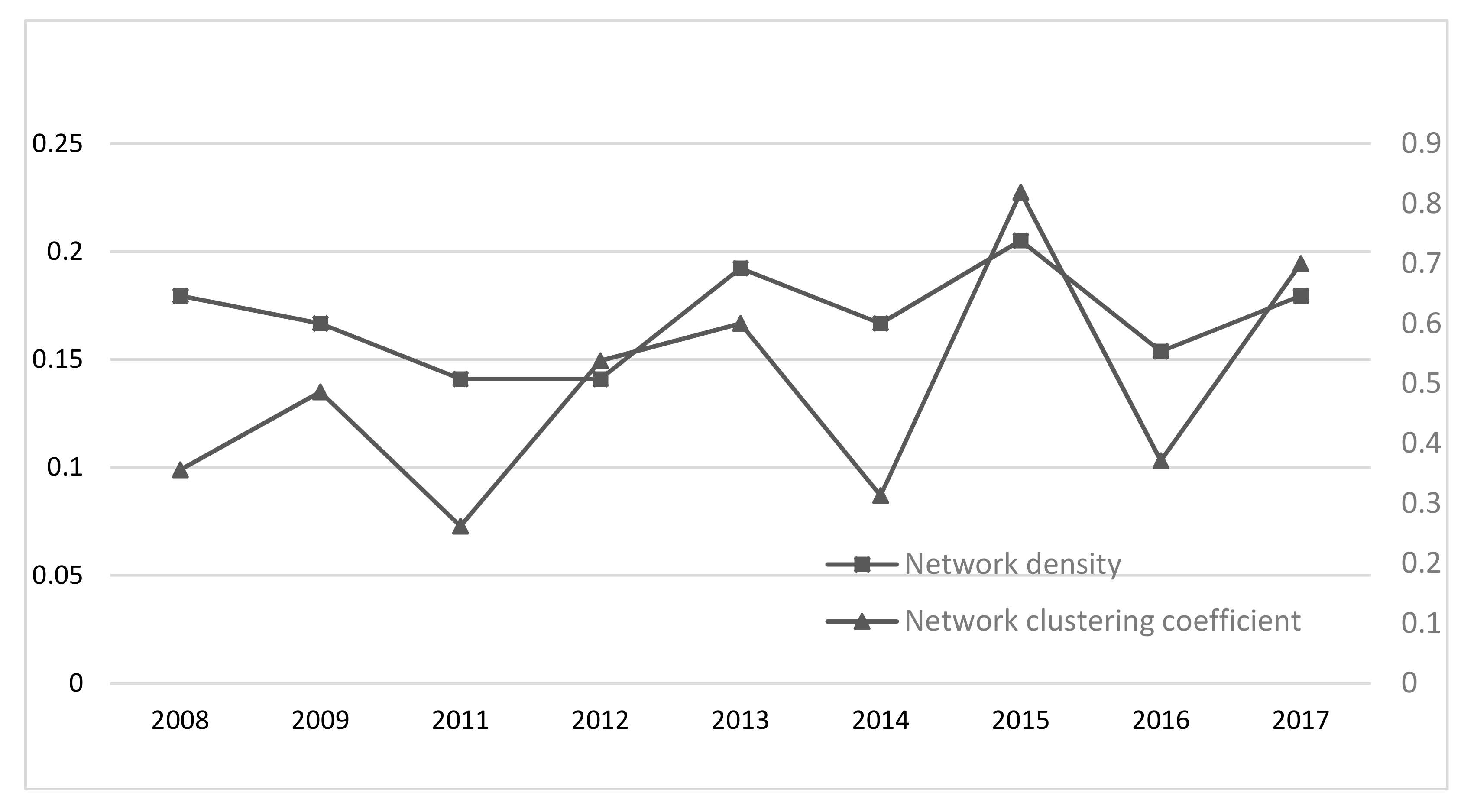
5.3. The Overall Law of Risk Evolution

In the above research, we analyzed the importance and relevance of financial risk indicators from the perspective of network nodes. Next, we further calculate the overall parameters of the network from the perspective of the overall risk network, based on the two dimensions of time and space, and analyze the evolution characteristics of the financial risk environment. From the time dimension, we can analyze the dynamic fluctuation trend of financial risks over time. From the spatial dimension, we can measure the risk contagion probability and contagion speed of each host country.

5.3.1. Time Law of Risk Evolution

We used the Ucinet software to calculate the network density and network clustering coefficient of complex networks in each year. The results are shown in Figure 4. As can be seen from the figure, the fluctuations of network density and clustering coefficient are relatively large. From 2008 to 2011, affected by financial crisis, the financial market was increasingly depressed, OFDI reduced, and the network density and clustering coefficient reached the bottom. After 2011, the impact of the financial crisis gradually receded and the financial market began to flourish. OFDI became more frequent, the network density and clustering coefficient ushered in a substantial increase, and then tended to be stable. Since 2016, the network density and clustering coefficient have tended to grow, indicating that under the trend of globalization, the financial risk environment has become increasingly complex, and the correlation between risks has increased. The change of a risk factor will lead to the rapid spread of risks and eventually lead to the outbreak of financial risks.

5.3.2. Spatial Law of Risk Evolution

Analysis of Risk Characteristics

We used the Ucinet software to calculate the network density and network clustering coefficient of complex networks in different countries. The results are shown in Table 6.
Network density indicates the tightness of the whole network connection. In terms of the network density of financial risk network, Pakistan, the United States, Israel have higher network density. It means that the financial risk environment of these countries is more complex and the risk is more closely related, that is, the risk has strong correlation; Clustering coefficient represents the degree of node clustering in the network. According to the results of clustering coefficient, the financial risk network in Pakistan, the United States, Israel have a high clustering coefficient, and both are greater than 0.5. This is consistent with the results of network density, indicating that the financial risk indicators in these countries are not only closely related, but also have a centralized trend, that is, the risk has a strong transitivity; The global efficiency of the network reflects the speed of risk evolution. From the results of the global efficiency of the network, Pakistan, the United States, Poland and other countries get higher rankings, indicating that when the host country has the same hidden risks, the risk spreads fastest in these countries.The analysis results based on network density, clustering coefficient and global efficiency show that under the same fluctuation of risk factors, the financial risk correlation in Australia, the United States, Israel, Poland and other countries is more complicated, the risk transitivity is stronger, and the investment in these countries is more likely to suffer financial risks.

Risk Transmission Path

After finding the important countries, in order to further analyze the relationship between financial risks among different countries, this paper constructs the MST to find the most possible transmission path of risk among countries. The basic principle of MST is based on greedy algorithm (a greedy algorithm means that when solving a problem, it always makes the best choice at the moment. That is to say, instead of considering the overall optimality, what it does is a local optimal solution in a certain sense). MST is a tree structure with n-1 edges formed by n nodes in a system. The edge set is the edge combination with the smallest weight and guarantees that no loop is formed, so MST has good robustness. In this paper, MST represents the strongest connection in the network. When MST is unique, it means it is the most possible risk transmission path in the financial network. That is, when a country’s financial environment is exposed to external shocks and risks occur, risk may spread to other countries along this risk transmission path at the fastest speed.
Before generating the MST, pearson correlation coefficient between country i and country j needs to be calculated. The calculation method is as follows:
p i , j = cov i , j σ i σ j
where cov denotes covariance, σi and σj denote the standard deviation.
Because the correlation coefficient does not satisfy the condition of metric space, this paper uses the practice of Mantegna [55] as a reference to convert the correlation coefficient into the distance between countries. The formulas is as follows:
d i , j = 2 1 p i , j
Then Kruskal’s algorithm is used to calculate the distance matrix, and the MST is obtained (the critical codes to generate MST are listed in Appendix A). The MST for 2017 is shown in Figure 5.
By analyzing the most possible transmission path of financial risk, we conclude the following characteristics: Firstly, the minimum spanning tree consists of 20 sample countries. According to the meaning of MST, we believe that the countries with more countries connected are the crucial countries for risk transmission. Therefore, Australia and Bulgaria are crucial countries for risk transmission among the 20 countries. Secondly, the MST of 20 countries can be roughly divided into four modules, For example, Bulgaria, Pakistan, Ukraine, and Zambia are combined to form a module, indicating that the financial risks of these four countries are closely related.
In addition, the length of the MST changes with time as shown in Figure 6. Generally, the shorter the length of the tree, the closer the relationship between countries. Figure 6 shows that after the 2008 financial crisis, the length of the tree was gradually decreasing, reaching a minimum in 2012. This shows that after the financial crisis, the financial market began to adjust. With the gradual recovery of the market, the links between countries became closer and closer, and the risk transmission was faster. After 2014, the length of the tree began to rise, indicating that the relationship between countries began to decline, and the path of financial risk transmission was longer, which was a good signal for OFDI enterprises.

6. Conclusions

Through theoretical study of complex network model, based on the empirical analysis framework of “theoretical analysis—model construction—variable selection—network parameters analysis”, this paper first constructs the the risk monitoring model of financial ecological environment. Through identifying the financial risk factors of OFDI, a risk indicator system including exchange rate risk, interest rate risk, capital market risk and financing risk is constructed. The financial risk data of 20 OFDI countries from 2008 to 2017 are selected as sample data for empirical analysis. By analyzing the characteristic parameters of the network model, the general laws of financial ecological environment risk in Chinese OFDI are obtained. The main conclusions of this paper are as follows:
The first is the importance of financial risk indicators of OFDI. M2/GDP, foreign exchange reserve, stock exchange turnover rate and total government debt as a percentage of GDP rank high in the degree centrality, indicating that these four risk indicators play an important role in the risk network and are the key nodes of risk evolution; At the same time, the result of closeness centrality is consistent with that of degree centrality, which means that these risk indicators are located at the core of the network and have strong independence. In addition, the betweenness centrality of the percentage of M2/GDP always ranks first, which is consistent with the result of degree centrality. It means that this indicator is not only closely related to other risk indicators, but also has a strong control effect on the whole financial risk network. However, the control ability of this indicator tends to weaken. Enterprises should focus on monitoring the fluctuations of the above indicators when conducting risk warnings.
The second is the relevance of financial risk indicators of OFDI. The following pairs of indicators are strongly correlated: Foreign exchange reserves, M2/GDP, and total government debt as a percentage of GDP (%); M2 growth and economic growth; inflation rates and non-performing loan ratio. These indicators should be monitored simultaneously. Usually, the abnormal fluctuation of one indicator will cause the change of another indicator, which will spread to the whole financial risk network and lead to the outbreak of financial risks.
The third is the overall evolution of financial risks on OFDI. In the time dimension, since 2016, network density and clustering coefficient have tended to grow, indicating that under the trend of globalization, the financial risk environment has become increasingly complex, the correlation between risks has increased. The change of a risk factor will lead to the rapid spread of risks and eventually lead to the outbreak of financial risks. In the spatial dimension, among the 20 sample countries, countries such as Pakistan, the United States and Israel have higher network density and clustering coefficient, which indicates that the financial risk within these countries is more complicated, risk transitivity is stronger, and the investment in these countries is more likely to suffer financial risks. Enterprises should avoid or be more cautious in choosing these countries as destination countries for OFDI, and the Chinese government should also increase its review of investment projects invested in these countries. The risk transmission path based on MST shows that Australia and Bulgaria are important countries for risk transmission. Since 2014, the length of risk transmission path has increased, that is, the path of financial risk transmission has been longer, which is a good signal for OFDI enterprises.
The contribution of this paper lies in introducing the method of complex network analysis into the study of OFDI financial risk, constructing the the monitoring model of financial risk evolution in an innovative manner, describing the general laws of inancial ecological environment risk in OFDI. The conclusions of this study have guiding significance for overseas investment companies to prevent investment risks and ensure their sustainable development overseas. Meanwhile, it can provide references for relevant departments to make policies. We acknowledge some limitations to our study. Due to the lack of complete data, we have to exclude some countries and only select 20 countries as samples. We believe that we could further extend the present study to enhance the credibility of the conclusion when the data becomes available.

Author Contributions

Conceptualization, J.M.; methodology, J.M.; software, J.Z.; formal analysis, J.M and J.Z.; writing: J.Z.; visualization, J.-B.Y.; supervision, J.-B.Y.; funding acquisition, J.M. All authors have read and agreed to the published version of the manuscript.

Funding

Fundamental Research Funds for the Central Universities: 2020VI032

Conflicts of Interest

The authors declare no conflict of interest.

Appendix A. The Critical Code to Generate MST

//Pearson correlation coefficient.
double PearsonCorrelation(vector<double> &A, vector<double> &B) {
//Check!
if(A.size() != B.size()) {
cout << “Error input!” << endl;
exit(-1);
}
 
//Calculate average value.
double sumA(0), sumB(0), aveA(0), aveB(0);
sumA = std::accumulate(A.begin(), A.end(), 0);
sumB = std::accumulate(B.begin(), B.end(), 0);
aveA = sumA/A.size();
aveB = sumB/B.size();
 
//Calculate correlation coefficient.
double Cov(0), VarA(0), VarB(0);
size_t length = A.size();
for (size_t i = 0; i < length; i++) {
Cov += (A[i]–aveA) * (B[i]–aveB);
VarA += pow((A[i]–aveA), 2);
VarB += pow((B[i]–aveB), 2);
}
 
return (Cov/sqrt(VarA * VarB));
}
 
//Find the connected component of vertex v.
int FindRoot(int parent[], int v) {
int s;
for(s = v; parent[s] >= 0; s = parent[s]);
while(s != v) {
int tmp = parent[v];
parent[v] = s;
v = tmp;
}
return s;
}
 
//Implementation of Kruskal’s algorithm
void Kruskal(Graph &G) {
int vex1, vex2;
double mstSum = 0;
 
int *parent = new int[G.m_vertexs.size()];
for(size_t i = 0; i < G.m_vertexs.size(); ++i) {
parent[i] = -1;
}
 
for(size_t num = 0, i = 0; i < G.m_edges.size(); ++i) {
vex1 = FindRoot(parent, G.m_edges[i].u);
vex2 = FindRoot(parent, G.m_edges[i].v);
if(vex1 != vex2) {
cout << “<“ << G.m_vertexs[G.m_edges[i].u].country << “-” << G.m_edges[i].u << “ --> “ << G.m_vertexs[G.m_edges[i].v].country << “-” << G.m_edges[i].v << “> : “ << G.m_edges[i].weight << endl;
mstSum += G.m_edges[i].weight;
parent[vex2] = vex1;
if(++num == G.m_vertexs.size()–1) {
cout << “The sum of the minimum spanning tree weights is:” << mstSum << endl;
break;
}
}
}
}
 
//Usage: you need to name the data file data.txt
int main() {
ifstream input(“data.txt”);
if(!input.good()) {
cerr << “Cann’t open file: “ << argv[1] << endl;
return -1;
}
 
//Build graph based on data content.
Graph G(input);
 
//Construction of minimum spanning tree using Kruskal’s algorithm.
Kruskal(G);
 
return 0;
}

Appendix B. Centrality Measurement Results
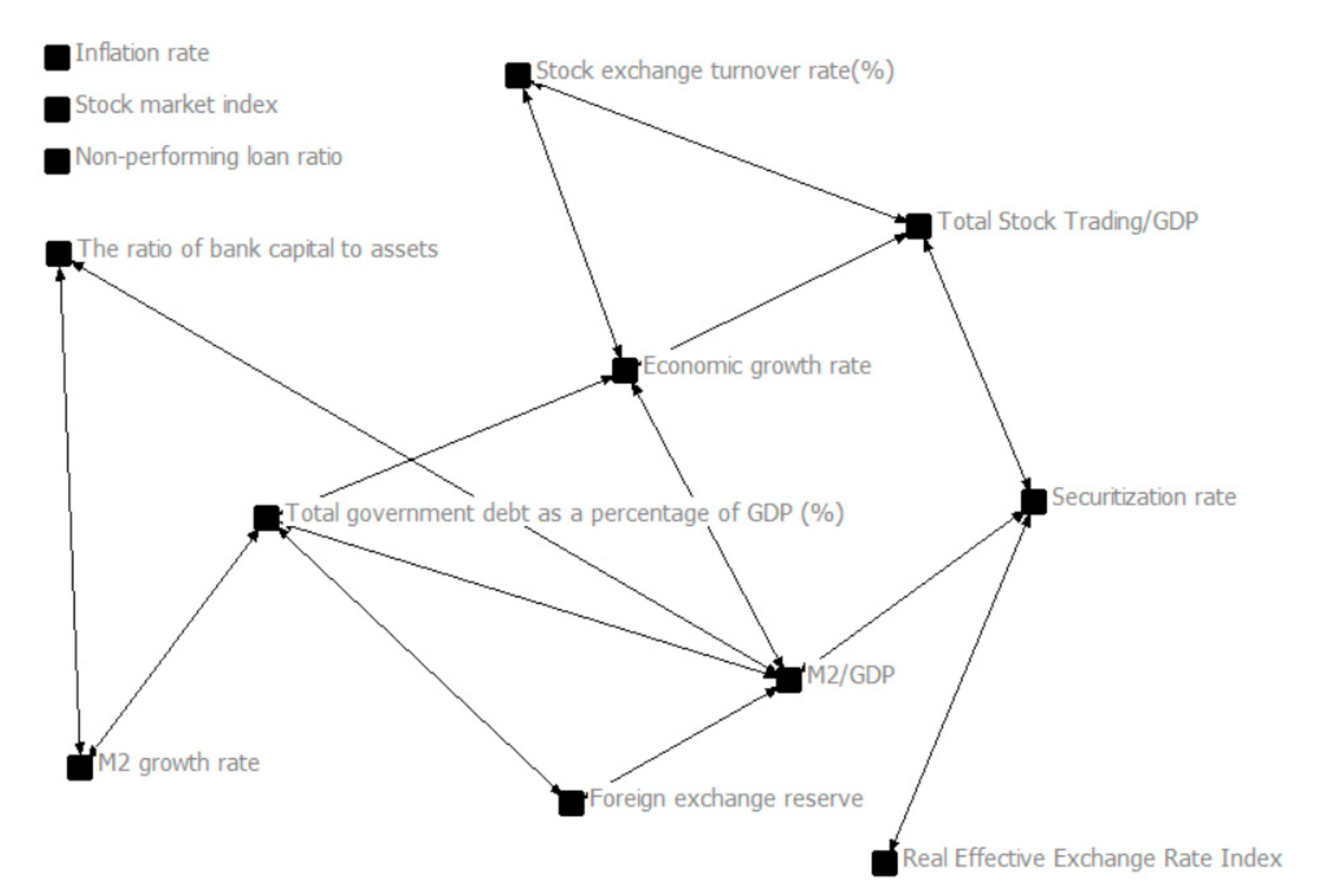
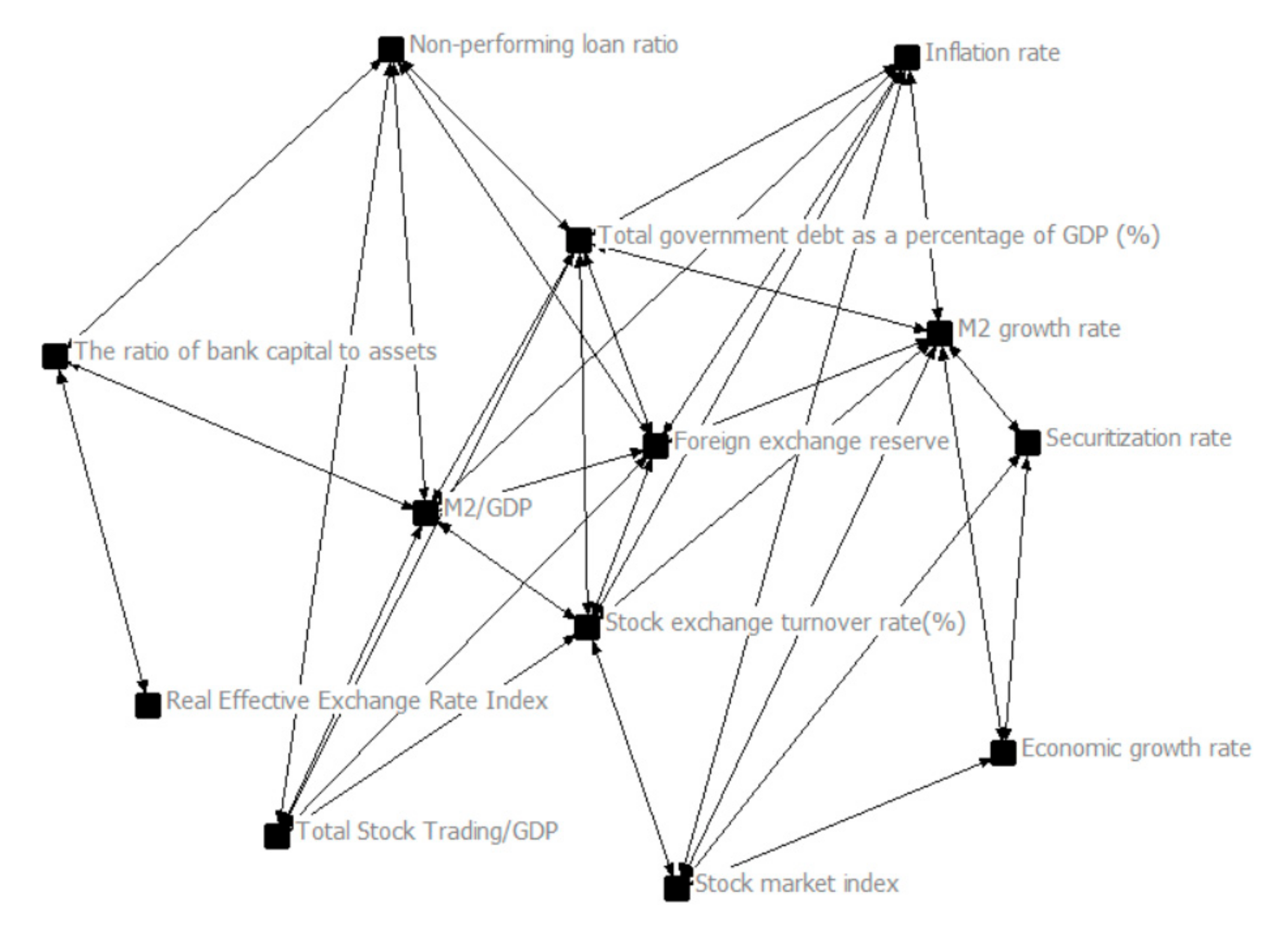
Table A1. Closeness centrality of financial risk network in 2008–2017.
Indicator Name200820092011201220132014201520162017
Real Effective Exchange Rate Index19.048 9.023 9.836 8.333
Foreign exchange reserve20.690 17.391 20.690 18.182 22.222 16.000 12.371 18.182 15.789
M2/GDP23.077 18.750 21.818 18.182 23.529 15.789 12.500 18.750 16.216
M2 growth rate20.000 8.333 19.672 16.901 19.672 8.333
Total government debt as a percentage of GDP (%)22.222 17.143 20.690 17.391 22.222 15.190 12.245 18.182 15.789
Inflation rate 18.462 20.339 16.667 21.053 9.917 17.391 15.385
Economic growth rate22.222 8.333 17.391 18.462 9.091 10.000
Stock market index 15.584 9.023 8.333 8.333
Total Stock Trading/GDP21.053 18.462 16.901 16.216 22.642 15.584 12.500 17.647 16.000
Securitization rate21.818 16.667 16.438 14.815 19.672 14.815 12.121 16.000 14.815
Stock exchange turnover rate (%)20.339 17.647 19.048 17.391 22.642 16.000 12.245 19.048 15.789
Non-performing loan ratio 17.143 18.462 15.190 9.917 17.647 14.286
The ratio of bank capital to assets20.690 16.667 20.339 14.634 16.901
Table A2. Betweenness centrality of financial risk network in 2008–2017.
Indicator Name200820092011201220132014201520162017
Real Effective Exchange Rate Index0.000 0.000 0.000 0.000 0.000 0.000 0.000 0.000 0.000
Foreign exchange reserve0.000 0.500 6.000 15.000 0.000 4.667 0.333 0.000 0.000
M2/GDP15.167 11.000 26.000 15.500 20.000 7.000 1.833 10.500 10.000
M2 growth rate0.500 0.000 8.000 0.500 0.000 0.000 0.000 0.000 0.000
Total government debt as a percentage of GDP (%)6.833 0.000 6.000 0.000 0.000 0.000 0.000 0.000 0.000
Inflation rate0.000 12.000 14.000 0.000 8.000 0.000 0.000 1.000 6.000
Economic growth rate8.667 0.000 0.000 0.000 0.000 1.000 2.000 0.000 0.000
Stock market index0.000 0.000 0.000 0.000 0.000 0.000 0.000 0.000 0.000
Total Stock Trading/GDP3.000 8.500 0.000 7.000 8.000 3.833 1.833 7.000 6.000
Securitization rate9.333 0.000 0.000 0.000 0.000 0.500 0.000 0.000 0.000
Stock exchange turnover rate (%)0.000 1.000 8.000 12.000 8.000 6.833 0.000 15.000 0.000
Non-performing loan ratio0.000 7.000 8.000 0.000 0.000 1.167 0.000 1.500 0.000
The ratio of bank capital to assets1.500 0.000 0.000 0.000 0.000 0.000 0.000 0.000 0.000
Table A3. Eigenvector centrality of financial risk network in 2008–2017.
200820092011201220132014201520162017
Real Effective Exchange Rate Index11.37700000000
Foreign exchange reserve40.34852.68969.48549.08459.2870.88261.99259.46361.102
M2/GDP70.63477.42869.68683.54265.45463.26469.25670.96864.369
M2 growth rate27.972028.32160.11214.7910000
Total government debt as a percentage of GDP (%)61.41439.3369.48544.37359.2842.25151.47659.46361.102
Inflation rate046.28428.92448.06316.520029.67316.676
Economic growth rate62.036010.05803.9330000
Stock market index04.6540000000
Total Stock Trading/GDP39.84560.320.0587.07962.12451.7369.25623.05164.166
Securitization rate37.23418.2274.1752.36914.79125.55435.5616.78815.636
Stock exchange turnover rate (%)31.1357.55656.47918.79162.12467.80551.47671.48461.102
Non-performing loan ratio015.39711.7550029.405029.794.064
The ratio of bank capital to assets30.130048.06315.58419.926020.90

References

  1. Carlson, D. Matrix Decompositions Involving the Schur Complement. Siam J. Appl. Math. 1975, 28, 577–587. [Google Scholar] [CrossRef]
  2. Goldberg, L.S.; Kolstad, C.D. Foreign Direct Investment, Exchange Rate Variability and Demand Uncertainty. Int. Econ. Rev. 1995, 36, 855–873. [Google Scholar] [CrossRef]
  3. Wang, H.J.; Qi, L. Country Economic Risks and FDI: Evidence from China. J. Financ. Econ. 2011, 10, 3–10. [Google Scholar]
  4. Levis, M. Does political instability in developing countries affect foreign investment flow? An empirical examination. Manag. Int. Rev. 1979, 19, 59–68. [Google Scholar]
  5. Darendeli, I.S.; Hill, T.L. Uncovering the complex relationships between political risk and MNE firm legitimacy: Insights from Libya. J. Int. Bus. Stud. 2016, 47, 68–92. [Google Scholar] [CrossRef]
  6. Globerman, S.; Shapiro, D.M. The impact of government policies on foreign direct investment: The Canadian experience. J. Int. Bus. Stud. 1999, 30, 513–532. [Google Scholar] [CrossRef]
  7. Egger, P.; Winner, H. How corruption influences foreign direct investment: A panel data study. Econ. Dev. Cult. Chang. 2006, 54, 459–486. [Google Scholar] [CrossRef]
  8. Alon, I.; Herbert, T.T. A stranger in a strange land: Micro political risk and the multinational firm. Bus. Horiz. 2009, 52, 127–137. [Google Scholar] [CrossRef]
  9. Liu, X.; Song, H.; Wei, Y.; Romilly, P. Country characteristics and foreign direct investment in China: A panel data analysis. Rev. World Econ. 1997, 133, 313–329. [Google Scholar] [CrossRef]
  10. Hayakawa, K.; Kimura, F.; Lee, H.H. How does country risk matter for foreign direct investment? Dev. Econ. 2013, 51, 60–78. [Google Scholar] [CrossRef] [Green Version]
  11. Schmidt, C.W.; Broll, U. Real exchange-rate uncertainty and US foreign direct investment: An empirical analysis. Rev. World Econ. 2009, 145, 513. [Google Scholar] [CrossRef]
  12. Takagi, S.; Shi, Z. Exchange rate movements and foreign direct investment (FDI): Japanese investment in Asia, 1987–2008. Jpn. World Econ. 2011, 23, 265–272. [Google Scholar] [CrossRef]
  13. Li, C.; Liu, H.; Jiang, Y. Exchange rate risk, political environment and Chinese outward FDI in emerging economies: A panel data analysis. Economics 2015, 3, 145–155. [Google Scholar]
  14. Altman, E.I.; Haldeman, R.G.; Narayanan, P. ZETATM analysis A new model to identify bankruptcy risk of corporations. J. Bank. Financ. 1977, 1, 29–54. [Google Scholar] [CrossRef]
  15. Miller, K.D. A framework for integrated risk management in international business. J. Int. Bus. Stud. 1992, 23, 311–331. [Google Scholar] [CrossRef]
  16. Lin, C.T.; Tsai, M.C. Location choice for direct foreign investment in new hospitals in China by using ANP and TOPSIS. Qual. Quant. 2010, 44, 375–390. [Google Scholar] [CrossRef]
  17. Memon, M.S.; Lee, Y.H.; Mari, S.I. Group multi-criteria supplier selection using combined grey systems theory and uncertainty theory. Expert Syst. Appl. 2015, 42, 7951–7959. [Google Scholar] [CrossRef]
  18. Duan, F.; Ji, Q.; Liu, B.Y.; Fan, Y. Energy investment risk assessment for nations along China’s Belt & Road Initiative. J. Clean. Prod. 2018, 170, 535–547. [Google Scholar]
  19. Sobczyk, E.J.; Kicki, J.; Sobczyk, W.; Szuwarzyński, M. Support of mining investment choice decisions with the use of multi-criteria method. Resour. Policy 2017, 51, 94–99. [Google Scholar] [CrossRef]
  20. Meldrum, D. Country risk and foreign direct investment. Bus. Econ. 2000, 35, 33–40. [Google Scholar]
  21. Thomas, D.E.; Grosse, R. Country-of-origin determinants of foreign direct investment in an emerging market: The case of Mexico. J. Int. Manag. 2001, 7, 59–79. [Google Scholar] [CrossRef]
  22. Al Khattab, A.; Anchor, J.; Davies, E. Managerial perceptions of political risk in international projects. Int. J. Proj. Manag. 2007, 25, 734–743. [Google Scholar] [CrossRef] [Green Version]
  23. Harris, R.S.; Ravenscraft, D. The role of acquisitions in foreign direct investment: Evidence from the U.S. Stock Market. J. Financ. 1991, 46, 825–844. [Google Scholar] [CrossRef]
  24. Kiymaz, H. The impact of country risk ratings on U.S. firms in large cross-border acquisitions. Glob. Financ. J. 2009, 20, 235–247. [Google Scholar] [CrossRef]
  25. Tarashev, N.A.; Borio, C.E.V.; Tsatsaronis, K. The Systemic Importance of Financial Institutions. BIS Q. Rev. 2009, 9, 75–87. [Google Scholar]
  26. Tobias, A.; Brunnermeier, M.K. CoVaR. Am. Econ. Rev. 2016, 106, 1705. [Google Scholar]
  27. Acharya, V.V.; Pedersen, L.H.; Philippon, T.; Richardson, M. Measuring Systemic Risk. Rev. Financ. Stud. 2017, 30, 2–47. [Google Scholar] [CrossRef]
  28. Brownlees, C.; Engle, R.F. SRISK: A Conditional Capital Shortfall Measure of Systemic Risk. Rev. Financ. Stud. 2017, 30, 48–79. [Google Scholar] [CrossRef]
  29. Karimalis, E.N.; Nomikos, N.K. Measuring systemic risk in the European banking sector: A Copula CoVaR approach. Eur. J. Financ. 2018, 24, 944–975. [Google Scholar] [CrossRef] [Green Version]
  30. Frankel, J.A.; Rose, A.K. Currency crashes in emerging markets:an empirical treatment. J. Int. Econ. 1996, 41, 35–66. [Google Scholar] [CrossRef] [Green Version]
  31. Sachs, J.; Tornell, A.; Velasco, A. Financial crises in emerging markets: The lessons from 1995. Natl. Bur. Econ. Res. 1996. [Google Scholar] [CrossRef]
  32. Kaminsky, G.; Lizondo, S.; Reinhart, C.M. Leading Indicators of Currency Crises; IMF Staff Paper: Washington, DC, USA, 1998; Volume 45. [Google Scholar]
  33. Illing, M.; Liu, Y. Measuring Financial Stress in a Developed Country: An Application to Canada. J. Financ. Stab. 2006, 2, 243–265. [Google Scholar] [CrossRef]
  34. Kumar, M.; Moorthy, U.; Perraudin, W. Predicting emerging market currency crashes. J. Empir. Financ. 2003, 10, 427–454. [Google Scholar] [CrossRef] [Green Version]
  35. Fioramanti, M. Predicting Sovereign Debt Crises Using Artificial Neural Networks:A Comparative Approach. J. Financ. Stab. 2008, 4, 164. [Google Scholar] [CrossRef]
  36. Ahn, J.J.; Oh, K.J.; Kim, T.Y.; Kim, D.H. Usefulness of support vector machine to develop an early warning system for financial crisis. Expert Syst. Appl. 2011, 38, 2966–2973. [Google Scholar] [CrossRef]
  37. Gandy, A.; Veraart, L.A. A Bayesian methodology for systemic risk assessment in financial networks. Manag. Sci. 2017, 63, 4428–4446. [Google Scholar] [CrossRef]
  38. Allen, F.; Gale, D. Financial contagion. J. Political Econ. 2000, 108, 1–33. [Google Scholar] [CrossRef]
  39. Gai, P.; Kapadia, S. Contagion in financial networks. Proc. R. Soc. A 2010, 466, 2401–2423. [Google Scholar] [CrossRef] [Green Version]
  40. Dastkhan, H.; Gharneh, N.S. How the ownership structures cause epidemics in financial markets: A network-based simulation model. Phys. A Stat. Mech. Appl. 2018, 492, 324–342. [Google Scholar] [CrossRef]
  41. León, C.; Machado, C.; Sarmiento, M. Identifying central bank liquidity super-spreaders in interbank funds networks. J. Financ. Stab. 2018, 35, 75–92. [Google Scholar] [CrossRef] [Green Version]
  42. Watts, D.J.; Strogatz, S.H. Collective dynamics of ‘small-world’networks. Nature 1998, 393, 440. [Google Scholar] [CrossRef] [PubMed]
  43. Barabási, A.L.; Albert, R. Emergence of scaling in random networks. Science 1999, 286, 509–512. [Google Scholar] [CrossRef] [PubMed] [Green Version]
  44. Chen, T.; He, J.; Li, X. An evolving network model of credit risk contagion in the financial market. Technol. Econ. Dev. Econ. 2017, 23, 22–37. [Google Scholar] [CrossRef]
  45. Zhang, J.; Wang, S.; Wang, X. Comparison analysis on vulnerability of metro networks based on complex network. Phys. A Stat. Mech. Appl. 2018, 496, 72–78. [Google Scholar] [CrossRef]
  46. Firth, J.A.; Sheldon, B.C.; Brent, L.J.N. Indirectly connected: Simple social differences can explain the causes and apparent consequences of complex social network positions. Proc. R. Soc. B Biol. Sci. 2017, 284, 20171939. [Google Scholar] [CrossRef] [PubMed] [Green Version]
  47. Nowzari, C.; Preciado, V.M.; Pappas, G.J. Analysis and control of epidemics: A survey of spreading processes on complex networks. IEEE Control Syst. Mag. 2016, 36, 26–46. [Google Scholar]
  48. Kim, J.; Rasouli, S.; Timmermans, H.J.P. Social networks, social influence and activity-travel behaviour: A review of models and empirical evidence. Transp. Rev. 2018, 38, 499–523. [Google Scholar] [CrossRef] [Green Version]
  49. Liu, N.; An, H.; Gao, X.; Li, H.; Hao, X. Breaking news dissemination in the media via propagation behavior based on complex network theory. Phys. A Stat. Mech. Appl. 2016, 453, 44–54. [Google Scholar] [CrossRef]
  50. Liu, C.; Arunkumar, N. Risk prediction and evaluation of transnational transmission of financial crisis based on complex network. Clust. Comput. 2019, 22, 4307–4313. [Google Scholar] [CrossRef]
  51. Erb, C.B.; Harvey, C.R.; Viskanta, T.E. Political risk, economic risk, and financial risk. Financ. Anal. J. 1996, 52, 29–46. [Google Scholar] [CrossRef] [Green Version]
  52. Alfaro, L.; Chanda, A.; Kalemli-Ozcan, S.; Sayek, S. FDI and economic growth: The role of local financial markets. J. Int. Econ. 2004, 64, 89–112. [Google Scholar] [CrossRef]
  53. Oet, M.V.; Bianco, T.; Gramlich, D.; Ong, S.J. SAFE: An early warning system for systemic banking risk. J. Bank. Financ. 2013, 37, 4510–4533. [Google Scholar] [CrossRef]
  54. Tao, L.; Zhu, Y. On China’s Financial Systemic Risks. J. Financ. Res. 2016, 6, 18–36. (In Chinese) [Google Scholar]
  55. Mantegna, R.N. Hierarchical structure in financial markets. Eur. Phys. J. B-Condens. Matter Complex Syst. 1999, 11, 193–197. [Google Scholar] [CrossRef] [Green Version]
Figure 1. Model construction ideas.
Sustainability 12 09456 g001
Figure 2. Financial risk network in 2008.
Sustainability 12 09456 g002
Figure 3. Financial risk network in Australia.
Sustainability 12 09456 g003
Figure 4. The density and clustering coefficient of financial risk network in 2008–2017.
Sustainability 12 09456 g004
Figure 5. Risk transmission path based on MST.
Sustainability 12 09456 g005
Figure 6. The trend of the MST length over time.
Sustainability 12 09456 g006
Table 1. Summary of representative studies of financial risk monitoring.
Author (Year) [Reference]ModelsCore ContentLimitations
Model method based on market dataTarashev et al. (2009) [25]Shapley valueMade full use of the theoretical basis of the game theory of Shapley value, individually consider the risk generated by each bank and its contribution to the risks of other banks in the system.Only the systematic importance of a single institution is considered.
Adrian and Brunnermeier (2016) [26]CoVaRExplored systemic financial risks from the risk spillover status of a single financial institution to other financial institutions and the entire financial market.The result is not additive.
Acharya et al. (2017) [27]SESIt measured the systemic risk impact on the economy that a single financial institution has been in trouble.Only applicable to post-event observation
MESIt examined the marginal contribution of a single institution to systemic financial risks under the circumstance of the decline in the overall market yield.
Brownlees and Engle (2017) [28]SRISKOn the basis of MES, the SRISK indicator (loss of financial institutions under the scenario of a certain drop in stock price) was constructed.Only pay attention to local interdependence
Karimalis and Nomikos (2018) [29]CopulaExamined common market factors that trigger systemic risk events.The issue of risk spillover between individual banks is not considered
Index method based on macro dataFrankel and Rose (1996) [30]FRAnalyzed the triggering factors of the financial crisis through historical data and judged the probability of the crisis.The degree of influence of various variables on the crisis cannot be directly measured.
Sachs et al. (1996) [31]STVSelected the cross-sectional data of 20 countries and used linear regression to establish an early warning model.Need to meet linear correlation conditions
Kaminsky et al. (1998) [32]KLRJudged the possibility of a financial crisis based on the number of warning indicators exceeding the threshold.The selection of the critical value has a great influence on the reliability of the results
Illing and Liu (2006) [33]FSISelected 11 relevant indicators of the stock market, bonds, banks and other markets to construct Canada’s comprehensive financial stress index.Unable to analyze the internal correlation between risks
Kumar, Moorthy and Perraudin (2002) [34]Simple LogitEarly warning model based on lagging macroeconomic and financial data.Indicators may have multicollinearity problems
Fioramanti (2008) [35]ANNA neural network early warning system with parameters and non-parameters was constructed, and the data of 46 developing countries from 1980 to 2004 were used to test the system.When there are many observation samples, the efficiency is not very high
Ahn, et al. (2011) [36]SVMTook the South Korean financial market as the research object, the SVM financial market risk early warning system is established.
Gandy and Veraart (2017) [37]Bayesian networkConstructed a financial network in the inter-bank market to measure the contagious effects of systemic financial risks.The premise is to assume that the attributes are independent of each other
Table 2. Financial risk indicator system.
First-Level Indicators Second-Level IndicatorsNumberData Sources
Exchange rate riskReal effective exchange rate indexX1WDI 1
Foreign exchange reserveX2EPS 2
M2/GDPX3WDI
M2 growth rateX4WDI
Interest rate riskTotal government debt as a percentage of GDP (%)X5Guo Yan Net 3
Inflation rateX6WDI
Economic growth rateX7WDI
Capital market riskStock market indexX8WDI
Total Stock Trading/GDPX9Sina Finance 4
Securitization rateX10Sina Finance
Stock exchange turnover rate (%)X11EPS
Financing riskNon-performing loan ratioX12WDI
The ratio of bank capital to assetsX13WDI
1 World Bank Database: https://data.worldbank.org.cn/indicator; 2 The full name of this database is Economy Prediction System and it is a professional data service platform founded by Beijing Focaste Information Technology Co., Ltd. (http://olap.epsnet.com.cn); 3 Founded in March 1998 and officially passed ISO9001:2000 quality management system certification on July 31, 2002. It is a famous professional economic information service platform in China (http://www.drcnet.com.cn/www/int/); 4 Sina Finance is a financial platform established in August 1999, providing timely stock price alerts and 24-hour global financial information services, as well as global market key data (https://finance.sina.com.cn/).
Table 3. Degree centrality of financial risk network in 2008–2017.
Indicator Name200820092011201220132014201520162017
Real Effective Exchange Rate Index100001101
Foreign exchange reserve233344434
M2/GDP554564555
M2 growth rate212310100
Total government debt as a percentage of GDP (%)423242334
Inflation rate032220222
Economic growth rate411012300
Stock market index010001101
Total Stock Trading/GDP341253525
Securitization rate311112211
Stock exchange turnover rate (%)233254354
Non-performing loan ratio022002221
The ratio of bank capital to assets200211010
Table 4. Clique of cohesive subgroups of financial risk indicators in 2008–2017.
Clique200820092011201220132014201520162017
1X2
X3
X4
X5
X13
X2
X3
X5
X9
X10
X11
X2
X3
X5
X9
X11
X2
X3
X4
X5
X6
X13
X2
X3
X5
X9
X10
X11
X3
X5
X6
X13
X2
X3
X5
X9
X10
X11
X2
X3
X5
X11
X13
X2
X3
X5
X9
X11
2X1
X7
X9
X10
X11
X4
X7
X13
X1
X4
X7
X13
X8
X9
X10
X11
X4
X6
X7
X1
X4
X7
X8
X4
X8
X13
X1
X4
X7
X8
X1
X7
X8
X10
3X6
X8
X12
X1
X6
X8
X12
X6
X8
X10
X12
X1
X7
X12
X1
X8
X12
X13
X2
X9
X10
X11
X12
X1
X6
X7
X12
X6
X9
X10
X12
X4
X6
X12
X13
Table 5. Density of cohesive subgroups of financial risk indicators in 2008–2017.
Clique200820092011
123123123
10.600.120.000.530.000.080.600.050.05
20.120.500.000.000.330.000.050.170.00
30.000.000.000.080.000.330.050.000.33
Clique201220132014
123123123
10.530.040.000.730.110.040.330.000.15
20.040.330.000.110.330.000.000.330.00
30.000.000.000.040.000.000.150.000.60
Clique201520162017
123123123
10.730.000.000.700.000.151.000.050.05
20.000.330.000.000.000.000.050.170.00
30.000.000.670.150.000.330.050.000.17
Table 6. Changes of basic statistical characteristics of OFDI financial risk network.
Country NameNetwork DensityClustering CoefficientGlobal Efficiency
Australia0.43210.7090.661
Pakistan0.62820.8190.812
Brazil0.43590.6820.688
Bulgaria0.26920.5550.469
Poland0.44870.6110.707
The Philippines0.43590.7760.564
Czech Republic0.34620.6030.624
Romania0.34620.6920.613
Malaysia0.37180.6520.588
The United States0.51280.7770.741
Mexico0.20510.4830.397
South Africa0.42310.6220.686
Nigeria0.34620.6300.567
Japan0.39740.7790.603
Saudi Arabia0.41030.6440.690
Ukraine0.34620.6850.553
Singapore0.43590.6250.641
Israel0.48720.9000.494
The United Kingdom0.43590.6050.692
Zambia0.23080.5870.441
Publisher’s Note: MDPI stays neutral with regard to jurisdictional claims in published maps and institutional affiliations.

