Transport of Contamination under the Influence of Sea Level Rise in Coastal Heterogeneous Aquifer

Abstract

This paper provided for the first time an experimental study on the influence of sea level rise on transport of contamination in the heterogeneous unconfined aquifer of the coastal zone. The experiments were conducted using the tank, considering the difference between sea level and inland head 1 cm for Case 1 and 2 cm for Case 2. Observed data were validated using the numerical model, which matched well with the toe length of seawater wedge and the shape of the contaminant plume. The results showed that the observed and simulated values of ${\mathrm{Cl}}^{-}$ concentration at the sampling points increased sharply at the initial time, and then they increased slowly and tended to be stable. The seawater wedge migrated inland with time under the effects of the hydraulic gradient toward the inland and the density difference between saltwater and freshwater. The steady state length of the 50% isoline of the seawater wedge was 167 cm in Case 2, which was larger than that of Case 1. The maximum area of plume in Case 2 was 0.13 m², larger than that in Case 1, which indicated that the velocity of diffusion of the contaminant plume increased as the sea level increased. As the velocity of diffusion increased, the time for pollutant migration to the intersection between seawater and freshwater became shorter. The maximum area and vertical depth of pollutant plume were sensitive to the hydraulic conductivity, dispersivity, and contamination concentration. The infiltration depth and range of the contaminant plume in the heterogeneous aquifer were greater than those in the homogeneous aquifer of the actual beach.

1. Introduction

The coastal area is densely populated, due to the rapid development of the economy there. Therefore, a large amount of groundwater is pumped to provide people with water for living and industrial production. Nevertheless, the problems of water resources, ecology, and environment pollution in coastal areas are complex and serious, due to the influences of interaction between land and sea, global warming, and sea level rising [1,2,3,4,5]. Among them, environmental pollution is a very serious problem. For example, the spilled oil deposits within the beach, caused by the accident of offshore oil tankers, which causes the long-term pollution of groundwater in the aquifer [6,7,8]. In addition, the wastewater infiltrates into the aquifer due to seepage from facilities, with the rapid development of the aquaculture in recent years, which results in the deterioration of groundwater quality and water balance of coastal aquifers [9,10,11]. Therefore, understanding the contaminate transport process and remediation in coastal groundwater is crucial to the economic, social, and environmental sustainability of coastal areas.

The spatial and temporal distribution of salinity in coastal zones have been focused on, because the seawater encroaches into the coastal aquifer e.g., [2,12,13,14,15,16]. In the recent decade, there has been increasing interests in the problem of seawater intrusion due to sea level rising, which is considered to be one of the most serious threats to the world’s freshwater resources [17,18,19,20,21]. The analytical e.g., [16,22,23], numerical e.g., [4,21,24], and experimental e.g., [18,25,26] methods have been used to study seawater intrusion caused by sea level rise. The seawater toe location and circulation rates of seawater under the condition of seawater level rising in the aquifers are investigated in previous studies.

The studies on coastal contaminant transport are relatively less, compared with those of seawater intrusion, because the movement of contaminant is inherently complex. The contaminant transport in the coastal aquifer is affected by many factors, such as the tide fluctuation, inland freshwater recharge, variable density flow, concentration of contaminant, and aquifer heterogeneity [27,28,29,30,31,32]. Among them, seawater intrusion has an important impact on pollutant transport, because the variable density effect can change the flow pattern and eventually affect the contaminant transport processes [33].

In previous studies, the methods of laboratory experiments, analytical solution, and numerical simulation were used to investigate the shape and movement of the solute plume in the coastal aquifer e.g., [7,33,34,35,36,37,38,39,40,41,42,43]. The laboratory experiment was applied to study the contaminant transport in the coastal aquifer earlier. For example, Zhang et al. [34] observed the landward plume transport during the experiment, which was affected by the tide fluctuation. Chang and Clement [38] investigated the contaminant transport patterns above the wedge and within it, and they found that the transport rate active was influenced by dispersion. Moreover, some analytical solutions were derived to explain the transport process directly. For instance, Koohbor et al. [33] derived a semi-analytical solution of pollutant transport in the coastal confined aquifer under the condition of variable velocity field. However, the analytical solution could be used to solve the pollutant transport problem under ideal conditions. The numerical simulation was applied to solve the problem of contaminant transport under the aforementioned complex conditions. Boufadel et al. [43] simulated the nutrient transport in the beach, and found that the solute transport was sensitive to tidal boundary condition and unsaturated parameters. Geng et al. [44] developed a numerical reactive transport model to simulate the fate and transport of the contaminant plume, which was influenced by tide amplitude, capillarity, and hydraulic conductivity. Shen et al. [32] considered the solute transport in beach aquifers, which was influenced by the unstable flow.

However, most of the previous studies focused on the contaminant transport in homogeneous aquifer. Up to now, several research studies on the contaminant transport in the heterogeneous aquifer were explored. In reality, the distribution of the plume was affected by the degree of heterogeneity of aquifer dramatically [7,45]. For example, Guo et al. [46] investigated the lithium tracer migration in a gravel beach with two-layered structure. Jang et al. [47] identified that the factor of soil heterogeneity affected the nitrate reduction process. Therefore, the heterogeneity of aquifers affecting the movement of pollutants in coastal aquifers should receive more attention. In addition, it was not clear how the rising sea level affects the contaminant transport in the heterogeneous aquifer, although there were many studies on the seawater intrusion caused by the rising sea level.

Fish ponds were built in the freshwater areas for aquaculture using the topography in coastal areas [10,48,49]. The seawater at the interface between saltwater and freshwater was pumped into the fish pond for aquaculture, and then the waste water was discharged to the sea. The infiltrated seawater caused by the leakage of aquaculture wastewater in the beach was an environmental pollution problem, which was different from the seawater intrusion caused by tide and artificial pumping. How does the seawater flow from the leakage of the fishpond in the aquifer? What is the relation between the infiltrated seawater from the fishpond and seawater intrusion from the sea? There was no research in this area so far. The aim of this paper is to explore the influence of sea level rise on contaminant transport in heterogeneous aquifers. The saltwater tracer is used to evaluate the contaminate transport in the heterogeneous aquifer, from the seepage of surface reservoirs. The complicated chemical and microbiological processes are not considered. The variation of the area and depth of contaminant under the condition of the rising sea level in the heterogeneous aquifer is examined, based on the laboratory experiments and numerical simulation. The effects of boundary condition, aquifer heterogeneity, and seawater intrusion on contaminant transport are discussed. The main hydrogeological factors affecting the contaminant transport in the coastal aquifer are determined.

2. Materials and Method

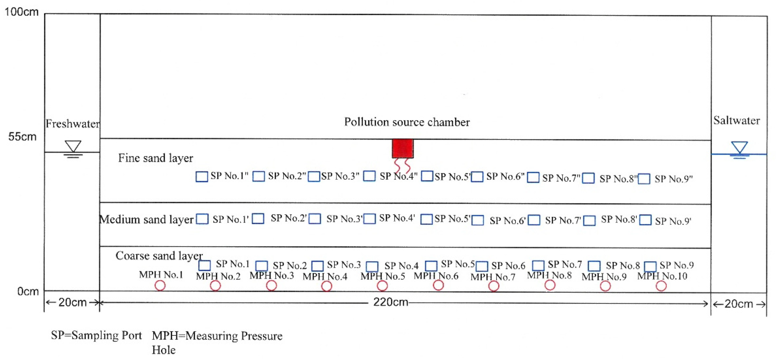
2.1. Laboratory Experiment

The dimension of the tank for experiment was 260 cm × 30 cm × 100 cm, which was shown in Figure 1. The tank was made of plexiglass and protected by a steel frame. It was composed of three parts: a freshwater chamber, a central chamber, and a seawater chamber. The left and right side chambers were separated from the central chamber by plates, which were made of PVC materials. In order to avoid the sand flowing from the central chamber to the two side chambers, the geotextile was pasted on the surface of the PVC board drilled with small holes. The bottom of the seawater chamber and freshwater chamber were respectively connected with a water reservoir, which was made of organic plastic plates with the length of 84 cm, width of 84 cm, and height of 84 cm. The seawater and freshwater were respectively pumped into the seawater chamber and freshwater chamber by peristaltic pumps. The left and right side chambers represented the freshwater and seawater boundary conditions, respectively. Three different particle sizes were used during the experiment, namely fine sand, medium sand, and coarse sand from up to down. The material was homogeneous in each layer. The particle sizes of fine sand, medium sand, and coarse sand were ranging from 0.1 to 0.25 mm, from 0.25 to 0.5 mm, and from 0.5 to 1 mm, respectively. The material in each layer was compacted. In reality, the coastal aquifer inclines to the sea boundary. However, the slope of the aquifer was generally small. Therefore, the slope of the aquifer for the experiment was set horizontal. The thickness of the surface sandy aquifer was generally larger, considering the actual beach condition. Therefore, the fine sand layer, medium sand layer, and coarse sand layer were laid horizontally in the sand tank, with the thickness of 23 cm, 16 cm, and 16 cm, respectively. The thickness of the whole aquifer was 55 cm. First of all, a certain amount of freshwater was put into the tank before filling the sand. Then, the coarse sand with the thickness of 2 cm was filled. The sand was left for 30 min to make it fully saturated. Subsequently, the above steps were repeated in turn until the coarse sand layer reach 16 cm. The method of laying sand in the medium sand layer and fine sand layer was similar to that of coarse sand. During the process of laying sand, each layer was compacted as much as possible to remove the air. The hydraulic conductivities of the fine sand, medium sand, and coarse sand were 2.3 × 10⁻⁵ m/s, 2.9 × 10⁻⁴ m/s, and 6.9 × 10⁻⁴ m/s, respectively, which were obtained from the variable head permeameters in the laboratory.

The pollution source chamber was installed on the top of the aquifer, which was 106 cm away from the left freshwater chamber. It was made by the transparent organic plastic plates, with the length of 30 cm, width of 5 cm, and height of 20 cm. A layer of geotextile was pasted at the bottom of the pollution source chamber drilled with holes, in order to prevent the sand from entering into the pollution source chamber. A peristaltic pump was used to pump the contaminant with constant concentration into the pollution source chamber at the constant speed. Ten pressure taps were arranged at the bottom of the sand box, and each tap was connected with a transparent polyurethane pipe to measure the variation of the groundwater level. A 0.2 mm filter screen was set at the pressure tap, in order to prevent the sand from entering the pressure pipe and blocking the pipe. At the back of the sand tank, there were nine sampling ports in each layer. The distance between each two sampling ports was 20 cm. During the experiment, the sample was taken from the sampling port using a syringe. Then, the water sample was diluted and the electrical conductivity of the sample was measured by the DDS-307 conductivity meter. The concentration of ${\mathrm{Cl}}^{-}$ can be calculated, because there is a linear relationship between the concentration of NaCl and electrical conductivity. Two sets of tests were considered for sea level rise. In the first experiment (Case 1), the left inland head and right sea level were fixed at 45 and 46 cm, respectively. In the second experiment (Case 2), the constant inland head and sea water level were maintained at 45 and 47 cm, respectively. The water level at different positions was observed at the measuring pressure holes during the experiment. The deionized water was used to make freshwater, and the density of freshwater was 1.0 × 10³ kg/m³. The concentration and density of saltwater were 35.0 g/L and 1.02 × 10³ kg/m³, respectively. The bright blue was added into the right seawater chamber, in order to show the seawater intrusion process. The saltwater with the concentration of 35.0 g/L was injected into the pollution source chamber. The carmine tracer with the concentration of 1.0 g/L was added into the saltwater to trace the movement of contaminant.

Each layer of the aquifer was filled with freshwater at the beginning of experiment. Then, the seawater flowed into the seawater chamber from the reservoir, and overflow was discharged through the overflow of the seawater chamber. Subsequently, the seawater gradually entered the water tank from the seawater chamber. The steady flow was formed on both sides. When the length of seawater wedge did not change in 5 min, the interface between seawater and freshwater reached steady state. Once the steady state was established, the peristaltic pump was open and the contaminant was injected into the pollution source chamber. The flow was set to 0.44 m/h, by controlling the peristaltic pump. At this time, the contaminant moved, influenced by the hydraulic gradient and density difference between seawater and freshwater. Finally, the experiment was finished when the contaminant plume intersected with the interface of seawater and freshwater in the coarse sand layer. The experimental process of Case 1 was similar to that of Case 2. During the experiment, the Canon digital camera (IXUS 175) was used to record the process of seawater wedge and contaminant migration. The salinity at each sampling port was monitored every 5 min. At the end of the experiment, the contaminant plume and saltwater wedge were analyzed by Matlab software.

2.2. Numerical Model and Procedure

Based on the finite difference model MODFLOW, the influence of density on groundwater flow was considered. A numerical simulation model of solute transport in groundwater flow was established by using SEAWAT [50,51]. The softwater was widely used in seawater intrusion and groundwater discharge e.g., [2,28,52,53,54]. The coupling controlling equations of groundwater flow and solute transport with variable density were as follows:

$$\begin{array}{l}\frac{\partial }{\partial x}\left[\rho K_{fx}\left(\frac{\partial h_f}{\partial x}+\frac{\rho -{\rho }_f}{{\rho }_f}\frac{\partial Z}{\partial x}\right)\right]+\frac{\partial }{\partial y}\left[\rho K_{fy}\left(\frac{\partial h_f}{\partial y}+\frac{\rho -{\rho }_f}{{\rho }_f}\frac{\partial Z}{\partial y}\right)\right]+\\ \frac{\partial }{\partial z}\left[\rho K_{fz}\left(\frac{\partial h_f}{\partial z}+\frac{\rho -{\rho }_f}{{\rho }_f}\frac{\partial Z}{\partial z}\right)\right]=\rho S_f\frac{\partial h_f}{\partial t}+\theta \frac{\partial \rho }{\partial C}\frac{\partial C}{\partial t}-{\rho }_s{q}_s\end{array}$$

(1)

$$\frac{\partial \theta C}{\partial t}=\nabla \left(\theta D\nabla C\right)-\nabla \left(\theta VC\right)+q_s{C}_s+R_n ,$$

(2)

where $\rho$ is the density of saline groundwater at a point in aquifer [ML⁻³]; ${\rho }_f$ is the density of fresh water [kg/m³]; $\rho$_s is density of water entering from a source or leaving through a sink [ML⁻³]; $q_s$ is the volumetric flow rate per unit volume of porous medium representing sources and sinks [T⁻¹]; $K_{fx},K_{fy},K_{fz}$ are the hydraulic conductivities in different directions [LT⁻¹]; Z is the position head [L]; $S_f$ is the specific storage [L⁻¹]; $h_f$ is the freshwater head [L]; $\theta$ is the effective porosity of porous medium [–]; C is the solute concentration [ML⁻³], and t is the time [T]; D is the hydrodynamic dispersion tensor [L²T⁻¹]; $C_s$ is the solute concentration of water entering or leaving from sources or sinks [M.L⁻³]; V is the fluid velocity vector [LT⁻¹]; and $R_n$ is reaction term of chemical substance.

The numerical simulation area was a heterogeneous and isotropic unconfined aquifer. During the setup of numerical simulation, the laboratory settings and parameters were followed as closely as possible. A two-dimensional vertical cross section was built, with the length of 220 cm and height of 55 cm. The domain of model was discretized into 24 layers and 5000 columns. A free surface boundary was defined on the upper part. A no-flow boundary condition was set on the bottom of the numerical model, because the bottom of the aquifer was bedrock in reality. For Case 1, the inland head and seawater level were set to 45 and 46 cm on the left and right boundaries, respectively. The left inland head and right seawater level were fixed at 45 and 47 cm for Case 2. The concentrations of saltwater and freshwater were set to 35 and 0 g/L, respectively. It was assumed that the contamination on the water table of the model was uniformly distributed at the distance between 1.04 and 1.08 m. The constant concentration of contamination was set to 35 g/L for Case 1 and Case 2. The injection time was at 55 and 50 min for Case 1 and Case 2, respectively. The simulated period was 110 min for Case 1 and 100 min for Case 2. The time step was set to 60 s for both cases.

In order to fit the observed head and salinity, the parameters of aquifers were calibrated repeatedly by a trial-and-error method. The process of calibration was to adjust the values of the parameters, including the hydraulic conductivities, specific yield, specific storage, effective porosity, and dispersivity, until the mean error between the calculated salinity values at the sampling ports was less than 10% of the maximum observed value variations. The horizontal hydraulic conductivity was assumed to be the same to its vertical value of the aquifer system. The estimated hydraulic conductivities were 4.6 × 10⁻⁵ m/s, 2.9 × 10⁻⁴ m/s, and 6.9 × 10⁻⁴ m/s, respectively, for the fine sand layer, medium sand layer, and coarse sand layer, respectively. The other parameters used in the simulations were listed in

Table 1. Model parameters and their values used in the numerical simulations.

Parameter	Definition	Unit	Value
K	Hydraulic Conductivity	m/s	4.6 × 10−5 (fine sand layer)
			2.9 × 10−4 (medium sand layer)
			6.9 × 10−4 (coarse sand layer)
µ	Specific Yield	-	0.2 (fine sand layer)
			0.25 (medium sand layer)
			0.30 (coarse sand layer)
$S_s$	Specific Storage	1/m	10−5
${\rho }_f$	Density of the Freshwater	kg/m3	1.0 × 103
$\rho$	Density of the Seawater	kg/m3	1.02 × 103
n	Porosity	-	0.3
${\alpha }_L$	Longitudinal Dispersivity	m	0.1
${\alpha }_T$	Transverse Dispersivity	m	0.01
$\tau D_m$	Molecular Diffusion Coefficient in Porous Media	m2/s	10−9
t	Time Period	min	110 for Case 1 100 for Case 2

.

3. Results and Discussion

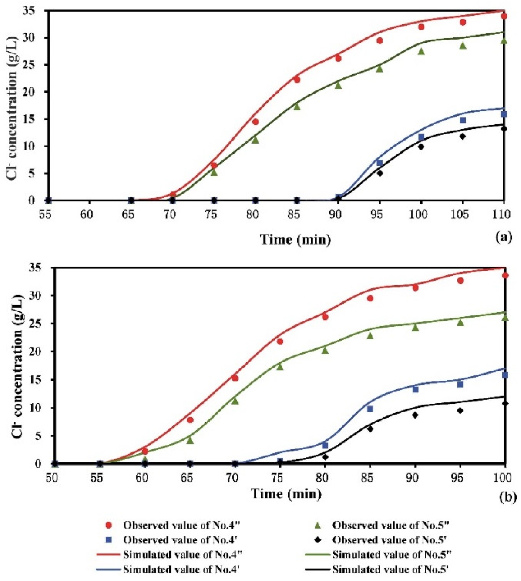
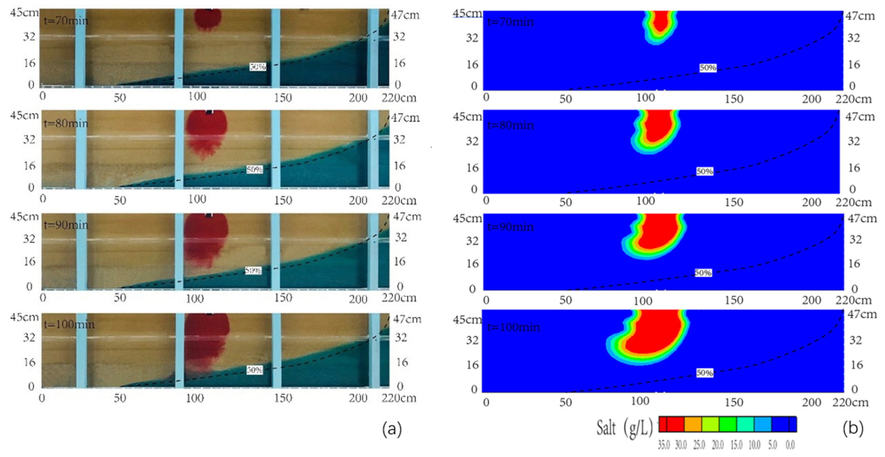
3.1. Numerical Validation

The numerical simulations of variable density groundwater flow and the solute transport model reproduced the observed water, ${\mathrm{Cl}}^{-}$ concentration, and contamination concentration in the transect. Here, the focus was on the ${\mathrm{Cl}}^{-}$ concentration. Figure 2 shows the experimental versus the simulated ${\mathrm{Cl}}^{-}$ concentrations variation with time at the four sampling points for Case 1 and Case 2. From the figure, one can see that the simulated and observed ${\mathrm{Cl}}^{-}$ exhibited good correlation generally. The calculated correlation coefficient (R²) ranged from 0.96 to 0.98, which indicated that the numerical model can successfully simulate the contaminant movement in the aquifer. From Figure 2, it can be seen that the observed and simulated values of ${\mathrm{Cl}}^{-}$ concentration increased sharply at the initial time, and then they increased slowly and tended to be stable.

The ${\mathrm{Cl}}^{-}$ concentration values at the sampling ports No. 4″ and No. 5″ in the upper layer were higher than those at No. 4′ and No. 5′ in the middle layer. It indicated that the concentration of contaminant decreased gradually when the contaminant plume migrated downward in the aquifer. The migration of plume in the medium sand layer lagged behind that in the fine sand layer. From Figure 2a, one can see that the maximum value of ${\mathrm{Cl}}^{-}$ concentration at left No. 4″ was close to 35 g/L, which was higher than that at right No. 5″ in the upper layer. The value of ${\mathrm{Cl}}^{-}$ concentration at left No. 4′ was higher than that at right No. 5′ in the middle layer, which was similar to that in the upper layer. It was evident that the distribution of contaminant was affected by the flow from the sea to inland. Compared with Figure 2a, Figure 2b showed that the values of concentration at the sampling points (No. 4″, No. 5″, No. 4′, and No. 5′) in Case 2 were little smaller than those in Case 1. It demonstrated that the contaminant was diluted due to the increase of water flow velocity influenced by the sea level rising.

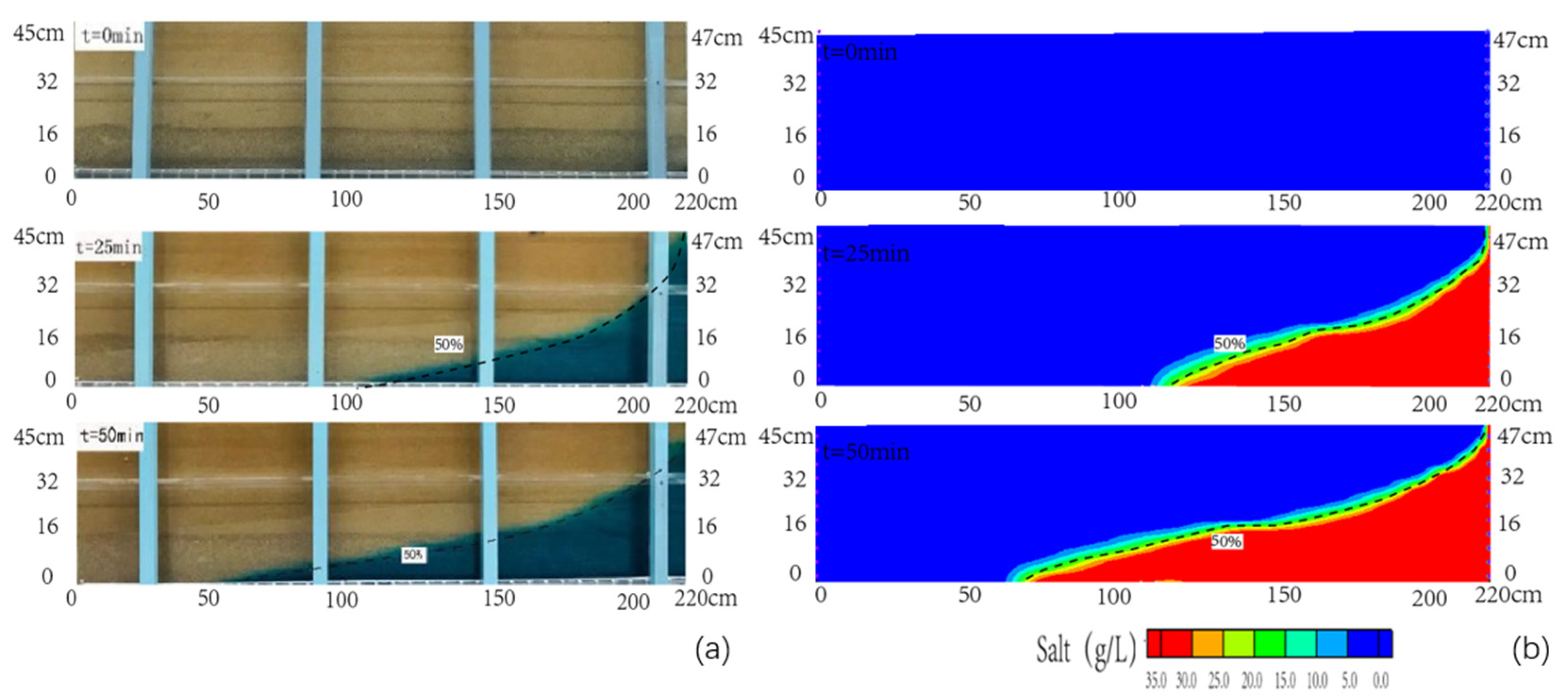
3.2. Seawater Intrusion Effected by Seawater Level Rise

In order to investigate the groundwater flow and salt transport under the influence of seawater level rising, simulations of seawater intrusion processes for different cases were conducted. Figure 3 reported the variation of observed data and simulated concentration color maps of the seawater wedge with time for Case 1. The comparison of Figure 3a,b reflected that the simulated toe lengths of the seawater wedge agreed with the observed ones well. The observed and simulated seawater wedge migrated inland with time, under the effects of the hydraulic gradient toward the inland and the density difference between saltwater and freshwater. The shape of the seawater wedge was parabolic. At the intial time, the migration velocity of the saltwater wedge was fast in the aquifer. The area increased in each layer of the aquifer. As for the hydraulic conductivity, the area and migration velocity of the seawater wedge increased from the top layer to bottom layer. Then, the migration velocity of the seawater wedge slowed down gradually, and it was close to zero when the time was 55 min. The interface of saltwater and freshwater reached equilibrium state, when the saltwater wedge did not move in the next five min. The toe position of 50% isoline of the seawater wedge represented the length of seawater wedge, which was wildly applied in depicting the saltwater wedge in the coastal aquifer, in which the dispersivity was small. As the invasion of seawater reaches the equilibrium status at the time of 55 min, the horizontal length of the 50% isoline of the observed seawater wedge can reach 142 cm. When the intruded seawater wedge was stable, the simulated length of the 50% isoline of seawater wedge was 144 cm, which was consistent with that of the observed seawater wedge.

Figure 4 showed the variation of observed data and simulated results of the toe position of seawater wedge at various time for Case 2. The seawater wedge encroached into the inland with time, which was influenced by the density difference between saltwater and freshwater and the hydraulic gradient slope toward the sea. Similar to Case 1, the shape of the seawater wedge was parabolic. The migration velocity of seawater intrusion was fast initially, and then it slowed down gradually in Case 2. The migration velocity of the seawater wedge was close to zero at the time of 50 min, and the steady state of seawater intrusion was formed at this time in the three layers. The observed length of the 50% isoline of the seawater wedge was 167 cm, which was larger than that of Case 1. It was because the head at the seaside boundary and the flow velocity for Case 2 were higher than those for Case 1. It reflected that the rising sea level had a positively impact on the seawater intrusion process in the layered aquifer, which was consistent with the observation in Guo et al. [18]. At the time of 50 min, the simulated length of 50% isoline of the seawater wedge was 167 cm (Figure 4b), which was consistent with the observed value (Figure 4a). In general, the numerical simulation model can describe the variation of the seawater wedge well.

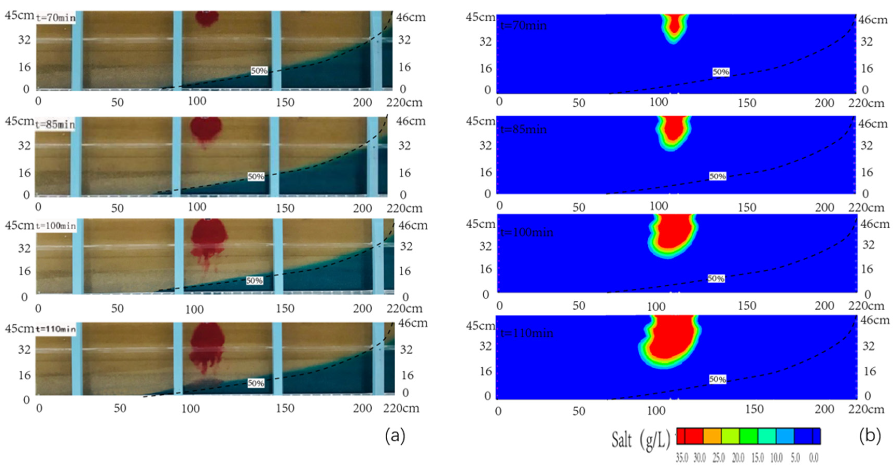
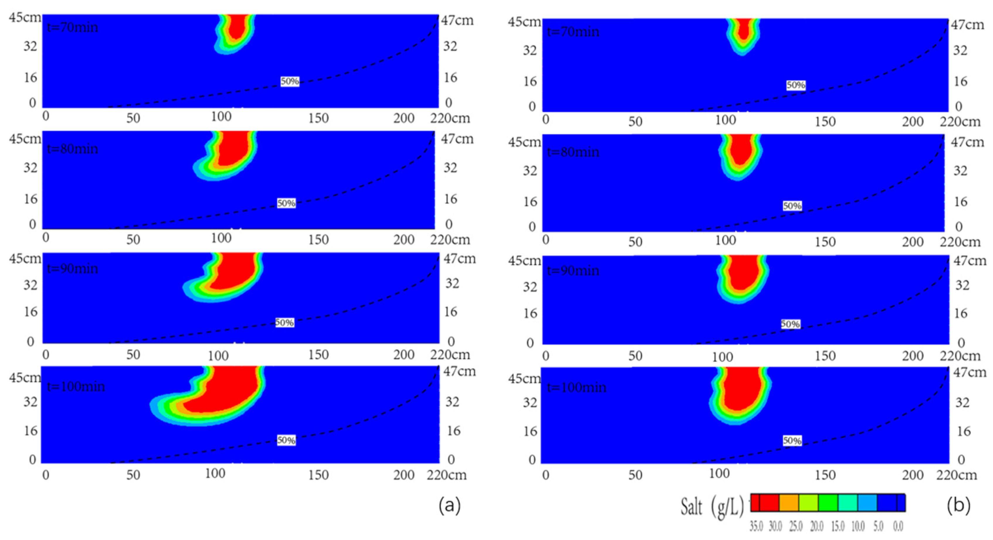
3.3. Contamination Transport Effected by Seawater Level Rise

The contaminate transport was simulated for both Case 1 and Case 2, when the seawater wedge was stable. Figure 5 showed the comparison between the observed and simulated contamination concentration at different times in the physical and numerical model for Case 1. The results showed that the numerical model could reproduce relatively well the overall shape of the plume, albeit the finger shape in the front of the plume observed in the laboratory was not captured in the simulation. The observed and simulated plume diffused mainly in the lateral and downward directions in the fine sand layer during the period of 55 and 70 min, and 70 and 85 min, respectively. The area of the contaminant plume increased linearly, and the shape of the plume was semi-elliptical. The maximum area of the contaminant plume was 0.02 m², and the maximum depth of the contaminant plume was 0.13 m. At the time of 85 min, the contaminant entered into the medium sand layer and moved downward. The pollution plume became concave at the interface between the upper layer and middle layer, because the velocity of the contaminant plume migration increased gradually. The contaminant plume migrated in the medium sand layer at the time between 85 and 100 min. The variation rate of area in the medium sand layer was twice as much as that of the fine sand layer. The maximum area of the contaminant plume was 0.067 m², and the maximum depth of the plume was 0.29 m. During the time of 100 and 110 min, the contaminant plume moved downward and inland in the coarse sand layer. The plume became concave at the interface between the middle layer and lower layer, due to the increasing of velocity of contaminant plume migration. The front of the pollutant flowed in the form of dominant flow, due to the heterogeneity in the coarse sand layer. The variation rate of the area in the coarse sand layer was 1.5 times of that in the middle sand layer, and the maximum plume area was 0.11 m² at the time of 110 min.

Figure 6 showed the comparison between the transient experimental and numerical contaminant transport for Case 2. In all, the results showed that the transient movement of the plume was reasonably well simulated by the numerical model, although the finger shape in the front of the plume observed in the laboratory was not captured in the simulation. During the period of 50 and 70 min, the observed and simulated plume diffused laterally in the fine sand layer. The area of the contaminant plume increased linearly, and the shape of the plume was semi-elliptical, which was similar to Case 1. The maximum area and depth of the contaminant plume were 0.025 m² and 0.13 m, respectively. At the time of 70 min, the contaminant entered into the medium sand layer and moved downward. The pollution plume became concave at the interface between the upper layer and middle layer, because the velocity of the contaminant plume migration increased gradually. The contaminant plume migrated in the medium sand layer at the time between 70 and 90 min. The maximum area of the contaminant plume was 0.069 m², and the maximum depth of plume was 0.29 m. During the time of 90 and 100 min, the contaminant plume moved downward and inland in the coarse sand layer. The plume became concave at the interface between the middle layer and lower layer, due to the increasing of velocity of contaminant plume migration. At the time of 100 min, the observed front of the pollutant was lower than that of the simulated one. Due to the heterogeneity in the coarse sand layer, the front of the pollutant flowed in the form of dominant flow. The variation rate of the area in the coarse sand layer was 2.0 times of that in the middle sand layer, and the maximum plume area was 0.13 m² at the time of 100 min. The end of the front of the contaminant plume migrated towards inland. Compared with the observed one, the numerical plume has a deviation toward the inland, because of the effect of seawater intrusion. Compared with Case 1, the area of the plume in Case 2 was larger than that in Case 1 in the same layer. It indicated that the velocity of diffusion of the contaminant plume increased as the sea level increased. As the velocity of diffusion increases, the time for the observed pollutant migration to the intersection between seawater and freshwater in Case 2 was shorter than that in Case 1.

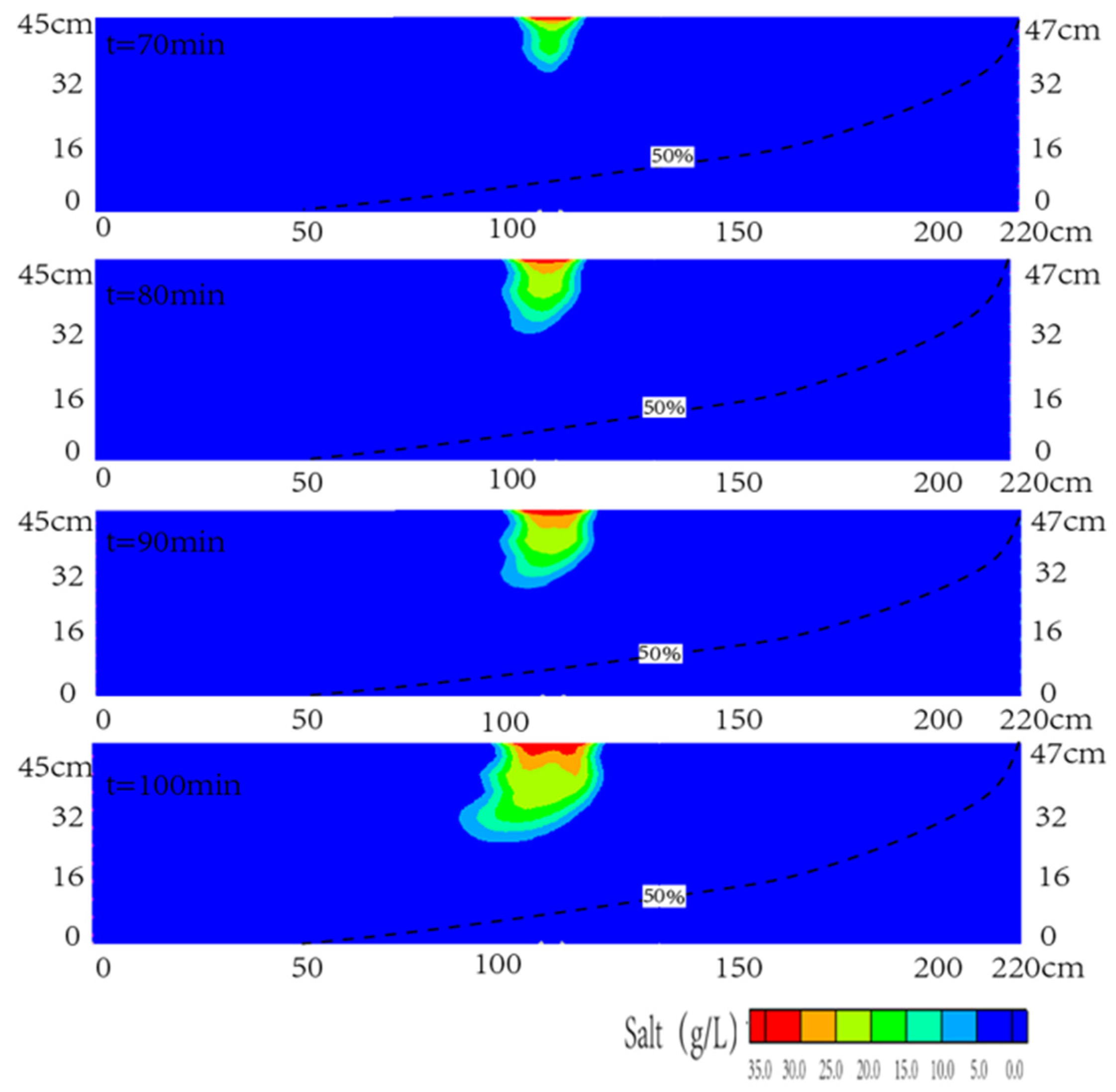
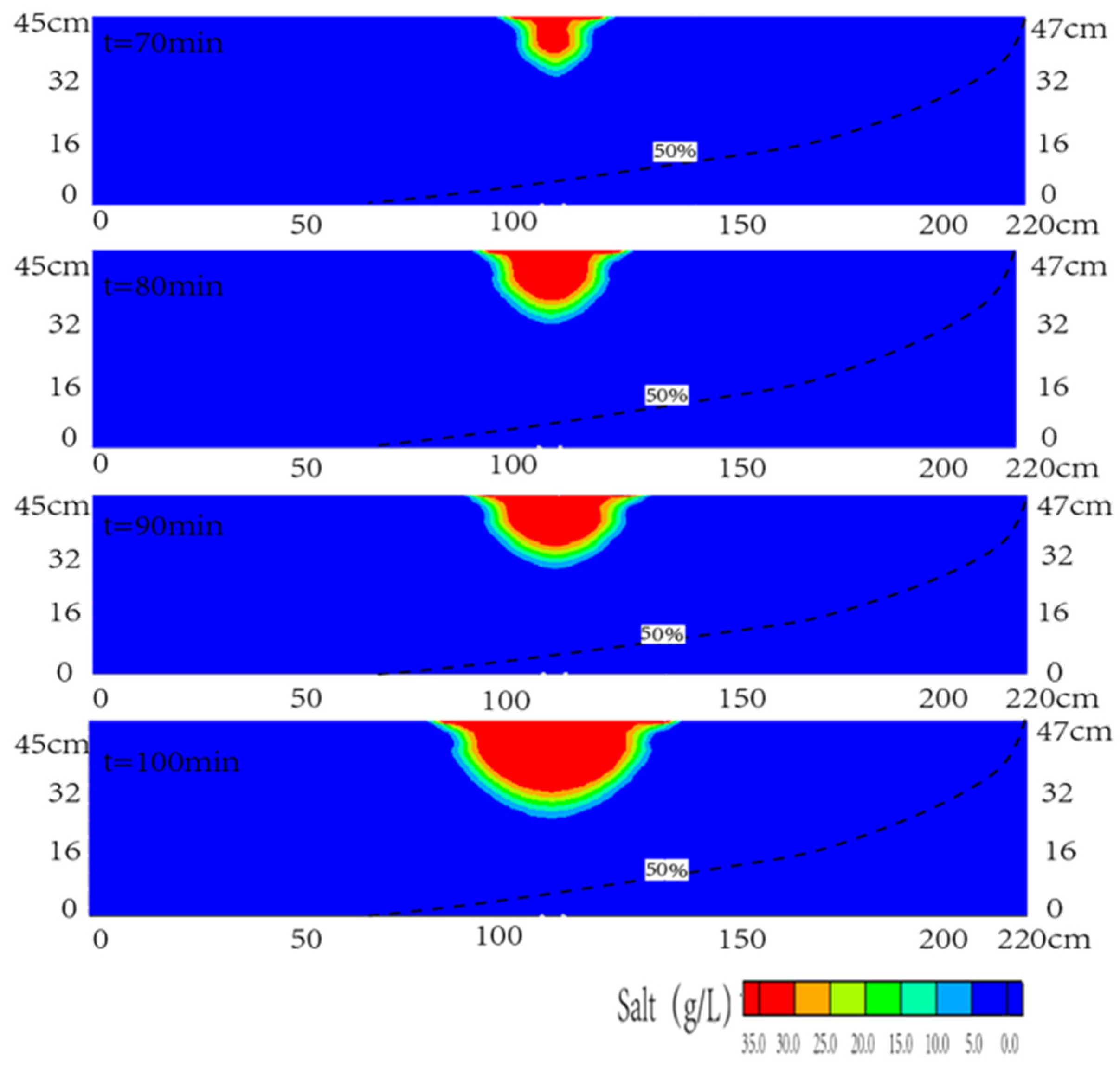
3.4. Sensitivity Analysis

The hydraulic conductivity, dispersivity, contaminate concentration, and heterogeneity were important parameters for solute transport in the coastal aquifer. Therefore, the sensitivities of saltwater contamination transported in the aquifer to the model parameters were analyzed, taking the Case 2 as an example. The area and velocity of the plume diffusion were discussed by changing the above parameters. It should be noted that the parameter values for analyzing the sensitivity were increased or decreased, whereas the values of the other parameters were not changed, which was shown in Table 1.

3.4.1. Effect of Hydraulic Conductivity

Figure 7a showed the simulated spatial contaminant plume distributions with time by the new model, as the values of K were raised to 8.0 m/d for the upper layer, 50.0 m/d for the middle layer, and 120.0 m/d for the bottom layer. Compared with Figure 6b, Figure 7a showed that the match to the observed contours of the saltwater contamination in the new model was worse, compared with the simulated ones in the Case 2. It was found that the larger length of the seawater wedge than in reality moved into the aquifer of the new model. The region of the transition zone in the front edge of the plume in the new model became larger, compared with that in the basic model. This was because the velocities were larger with higher hydraulic conductivities. The plume migrated more downward and landward, especially in the coarse sand layer. Increasing the hydraulic conductivity increased remarkably the area of the plume in the heterogeneous aquifer. The maximum area of the pollution plume simulated by the new model reached 0.143 m², which was larger than that simulated in Case 2.

As the values of K were reduced to 2.0 m/d for the upper layer, 12.5 m/d for the middle layer, and 30.0 m/d for the bottom layer, Figure 7b showed that the match to the observed contours of the saltwater contamination was considerably worse, compared with the simulated ones in Figure 6b of Case 2. One can see that the smaller length of the seawater wedge than in reality migrated into the aquifer of the new model. Obviously, the maximum vertical pollution depth decreased when the hydraulic conductivities of the heterogeneous aquifer decreased, which indicated that the hydraulic conductivities for sensitivity analysis were too low. Additionally, with the lower hydraulic conductivities in each layer, the velocity of plume migration became slowly. However, the migration direction of the pollution plume remained downward and landward. The area of the pollution plume simulated by the new model increased slowly, and the maximum value of it reached 0.083 m², which was smaller than that of Case 2. Therefore, one can conclude that increasing or decreasing the hydraulic conductivities by the new models were not able to reproduce the spatial distributions of saltwater contamination concentration.

3.4.2. Effect of Dispersion

The sensitivity of the plume transport to the dispersivity was explored for two new models, due to the importance of dispersivity for solute transport. The variation of contours of the saltwater contamination was used for analyzing sensitivity with respect to the dispersivity. When the value of ${\alpha }_L$ increased to 0.5 m and the ratio ${\alpha }_T/{\alpha }_L$ was 0.1, Figure 8a showed that more saltwater intruded into the aquifer of the new model than that of the basic case. The length of seawater in the new model was 0.13 m longer than that in Case 2. The simulated maximum vertical pollution depth was larger, compared with that in the basic model, which could be because high dispersivity induced widening of the transition zone. The area of the pollution plume simulated by the new model was 0.163 m², which was larger than that of Case 2. It indicated that higher dispersion has great influence on plume transport. However, there was no change in the direction of pollutant migration.

When the value of ${\alpha }_L$ decreased to 0.01 m and the ratio ${\alpha }_T/{\alpha }_L$ was 0.1, Figure 8b showed that the area simulated by the new model could not match the observed ones at different times, compared with Figure 6b. The length of seawater in the new model was 0.093 m smaller than that in Case 2. It depicted that the area of pollution plume simulated by the new model was 0.086 m², which was much smaller than that of Case 2. It indicated that decreasing the dispersion would lead to the slow migration velocity of plume. Overall, changes in dispersivity have effects on plume transport.

3.4.3. Effect of Contaminant Concentration

The saltwater concentration was reduced from 35 to 20 g/L in the new model. Figure 9 shows that the fitting to the observed plume was worse, compared with that of the basic case in Figure 6b. One can see that the area of the pollutant plume and maximum vertical pollution depth decreased sharply, whereas the movement of the plume decreased slightly in the horizontal direction of the new model, compared with the simulated ones in Case 2. It was because the dispersion was too small. At the time of 100 min, the simulated area of the plume was 0.063 m², which was smaller than that of the basic case. However, the direction of the pollutant plume migration was downstream and landward in the aquifer. Therefore, the range of the plume was sensitive to the concentration of contamination.

3.4.4. Effect of Homogeneous Aquifer

In order to discuss the influence of heterogeneity on the contamination transport, numerical contamination simulation in the homogeneous aquifer was considered. The aquifer was assumed to be filled with fine sand based on Case 2. The value of K of the whole aquifer was taken as 4.0 m/d, and the other parameters were fixed as shown in Table 1. Figure 10 showed the simulated contamination concentration distributions of the cross section in the homogeneous aquifer for the new model. The steady state length of the seawater in the new model was smaller than that in Case 2. At the time of 70 min, the shape of the pollution plume was semi-elliptic, which was the same to that of the basic case. Then, the plume migrated downward and laterally during the period between 70 to 100 min, compared to that of the basic case. The vertical migration of the plume decreased, nevertheless, the movement in the horizontal direction increased slightly for the new model. This was because the vertical velocity of the new model was smaller than that of the basic case. There was no concave observed in the plume during the process of pollutant transport, compared to Figure 6b. At the time of 100 min, the maximum area and vertical pollution depth of the pollutant plume reached 0.11 m² and 0.25 m in the new model, which were smaller than those simulated by the basic case. Therefore, one can conclude that the infiltration depth and range of the contaminant plume in the heterogeneous aquifer were greater than those in the homogeneous aquifer of the actual beach.

4. Conclusions

This paper presented for the first time analyzing the influence of sea level rise on contaminate transport in the heterogeneous unconfined aquifer of the coastal zone. Two sets of laboratory experiments were tested considering the rising sea level (the difference between sea level and inland head was 1 cm for Case 1 and 2 cm for Case 2). The variation of seawater intrusion and contaminant transport with time were observed during both sets of experiments. The numerical model SEAWAT was used for validation. The numerical results of the model provided matched well with the experimental data for both the toe length of seawater wedge and the shape of the contaminant plume for the rising sea level in the heterogeneous unconfined aquifer.

The observed and simulated values of ${\mathrm{Cl}}^{-}$ concentration at the sampling points increased sharply at the initial time, and then they increased slowly and tended to be stable. The ${\mathrm{Cl}}^{-}$ concentration in the medium sand layer was smaller than that in the fine sand layer, which indicated that the migration of plume in the middle layer lagged behind that in the upper layer. The values of concentration at the sampling points in Case 2 were a little smaller than those in Case 1, because the contaminant was diluted due to the increase of water flow velocity influenced by the rising sea level. The observed and simulated seawater wedge migrated inland with time, under the effects of the hydraulic gradient toward the inland and the density difference between saltwater and freshwater. The steady state length of the 50% isoline of the seawater wedge was 167 cm in Case 2, which was larger than that of Case 1. It was because the head at the seaside boundary and the flow velocity for Case 2 were higher than those for Case 1.

In both cases, the observed and simulated plume diffused laterally and downward in the fine sand layer and medium sand layer. The contaminant plume moved downward and inland in the coarse sand layer. The front of the pollutant flowed in the form of the dominant flow, due to the heterogeneity of the aquifer. At the interface between each two layers, the plume became concave due to the increasing velocity of contaminant plume migration. The maximum area of plume in Case 2 was 0.13 m², larger than that in Case 1, which indicated that the velocity of diffusion of the contaminant plume increased as the sea level increased. As the velocity of diffusion increased, the time for pollutant migration to the intersection between seawater and freshwater became shorter. The maximum area and vertical depth of the pollutant plume were sensitive to the hydraulic conductivity, dispersivity, and contamination concentration. The infiltration depth and range of the contaminant plume in the heterogeneous aquifer were greater than those in the homogeneous aquifer of the actual beach.

References

1. Ferguson, G.; Gleeson, T. Vulnerability of coastal aquifers to groundwater use and climate change. Nat. Clim. Chang. 2012, 2, 342–345. [Google Scholar] [CrossRef]
2. Guo, Q.N.; Huang, J.W.; Zhou, Z.F.; Wang, J.G. Experiment and numerical simulation of seawater intrusion under the influences of tidal fluctuation and groundwater exploitation in coastal multilayered aquifers. Geofluids 2019, 2019, 2316271. [Google Scholar] [CrossRef] [Green Version]
3. Post, V.E.A. Fresh and saline groundwater interaction in coastal aquifers: Is our technology ready for the problems ahead. Hydrogeol. J. 2005, 13, 120–123. [Google Scholar] [CrossRef]
4. Sefelnasr, A.; Sherif, M. Impacts of seawater rise on seawater intrusion in the Nile Delta aquifer, Egypt. Ground Water 2014, 52, 264–376. [Google Scholar] [CrossRef] [PubMed]
5. Werner, A.D.; Bakker, M.; Post, V.E.A.; Vandenbohede, A.; Lu, C.H.; Ataie-Ashtianiab, B.; Simmons, C.T.; Barry, D.A. Seawater intrusion processes, investigation and management: Recent advances and future challenges. Adv. Water Resour. 2013, 51, 3–26. [Google Scholar] [CrossRef]
6. Guo, Q.N.; Li, H.L.; Boufadel, M.C.; Sharifi, Y. Hydrodynamics in a gravel beach and its impact on the Exxon Valdez oil. J. Geophys. Res. 2010, 115. [Google Scholar] [CrossRef] [Green Version]
7. Li, H.L.; Boufadel, M.C. Long-term persistence of oil from the Exxon Valdez spill in two-layer beaches. Nat. Geosci. 2010, 3, 96–99. [Google Scholar] [CrossRef]
8. Boufadel, M.; Geng, X.L.; An, C.J.; Owens, E.; Chen, Z.; Lee, K.N.; Taylor, E.; Prince, R.C. A Review on the factors affecting the deposition, retention, and biodegradation of oil stranded on beaches and guidelines for designing laboratory experiments. Curr. Pollut. Rep. 2019, 5, 407–423. [Google Scholar] [CrossRef]
9. Herbeck, S.L.; Unger, D.; Wu, Y.; Jennerjahn, C.T. Effluent, nutrient and organic matter export from shrimp and fish ponds causing eutrophication in coastal and back-reef waters of NE Hainan, tropical China. Cont. Shelf Res. 2013, 57, 92–104. [Google Scholar] [CrossRef]
10. Tal, A.; Weinstein, Y.; Yechieli, Y.; Borisover, M. The influence of fish ponds and salinization on groundwater quality in the multi-layer coastal aquifer system in Israel. J. Hydrol. 2017, 551, 768–783. [Google Scholar] [CrossRef]
11. Tal, A.; Weinstein, Y.; Walman, S.; Goldman, M.; Yechieli, Y. The interrelations between a multi-layered coastal aquifer, a surface reservoir (fish ponds) and the sea. Water 2018, 10, 1426. [Google Scholar] [CrossRef] [Green Version]
12. Abd-Elhamid, H.F.; Javadi, A.A. Impact of sea level rise and over-pumping on seawater intrusion in coastal aquifers. J. Water Clim. Chang. 2011, 2, 19–28. [Google Scholar] [CrossRef]
13. Anwar, N.; Robinson, C.; Barry, D.A. Influence of tides and waves on the fate of nutrients in a nearshore aquifer: Numerical simulations. Adv. Water Resour. 2014, 73, 203–213. [Google Scholar] [CrossRef]
14. Ataie-Ashtiani, B.; Volker, R.E.; Lockington, D.A. Tidal effects on seawater intrusion in unconfined aquifers. J. Hydrol. 1999, 216, 17–31. [Google Scholar] [CrossRef]
15. Ataie-Ashtiani, B.; Werner, A.D.; Simmons, C.T.; Morgan, L.K.; Lu, C. How important is the impact of land-surface inundation on seawater intrusion caused by sea-level rise? Hydrogeol. J. 2013, 21, 1673–1677. [Google Scholar] [CrossRef]
16. Lu, C.; Xin, P.; Li, L.; Luo, J. Seawater intrusion in response to sea-level rise in a coastal aquifer with a general-head inland boundary. J. Hydrol. 2015, 522, 135–140. [Google Scholar] [CrossRef]
17. Green, N.R.; MacQuarrie, K.T.B. An evaluation of the relative importance of the effects of climate change and groundwater extraction on seawater intrusion in coastal aquifers in Atlantic Canada. Hydrogeol. J. 2014, 22, 609–623. [Google Scholar] [CrossRef]
18. Guo, Q.N.; Zhang, Y.H.; Zhou, Z.; Zhao, Y. Saltwater transport under the influence of sea-level rise in coastal multilayered aquifers. J. Coast. Res. 2020, 36, 1040–1049. [Google Scholar] [CrossRef]
19. Ketabchi, H.; Mahmoodzadeh, D.; Ataie-Ashtiani, B.; Simmons, C.T. Sea-level rise impacts on seawater intrusion in coastal aquifers: Review and integration. J. Hydrol. 2016, 535, 235–255. [Google Scholar] [CrossRef]
20. Lemieux, J.M.; Hassaoui, J.; Molson, J.; Therrien, R.; Therrien, P.; Chouteau, M.; Ouellet, M. Simulating the impact of climate change on the groundwater resources of the Magdalen Islands, Quebec, Canada. J. Hydrol. Reg. Stud. 2015, 3, 400–423. [Google Scholar] [CrossRef] [Green Version]
21. Mehdizadeh, S.S.; Karamalipour, S.E.; Asoodeh, R. Sea level rise effect on seawater intrusion into layered coastal aquifers (simulation using dispersive and sharp-interface approaches). Ocean Coast. Manag. 2017, 138, 11–18. [Google Scholar] [CrossRef]
22. Ketabchi, H.; Mahmoodzadeh, D.; Ataie-Ashtiani, B.; Werner, A.D.; Simmons, C.T. Sea-level rise impact on fresh groundwater lenses in two-layer small islands. Hydrol. Process. 2014, 28, 5938–5953. [Google Scholar] [CrossRef]
23. Shi, W.L.; Lu, C.H.; Ye, Y.; Wu, J.C.; Li, L.; Luo, J. Assessment of the impact of sea-level rise on steady-state seawater intrusion in a layered coastal aquifer. J. Hydrol. 2018, 563, 851–862. [Google Scholar] [CrossRef]
24. Webb, M.D.; Howard, W.F. Modeling the transient response of saline intrusion to rising sea levels. Groundwater 2011, 49, 560–569. [Google Scholar] [CrossRef] [Green Version]
25. Abdoulhalik, A.; Ahmed, A.A. Transience of seawater intrusion and retreat in response to incremental water-level variations. Hydrol. Process. 2018, 32, 2721–2733. [Google Scholar] [CrossRef]
26. Morgan, L.K.; Stoeckl, L.; Werner, A.D.; Post, V.E.A. An assessment of seawater intrusion overshoot using physical and numerical modeling. Water Resour. Res. 2013, 49, 6522–6526. [Google Scholar] [CrossRef]
27. Ataie-Ashtiani, B.; Volker, R.E.; Lockington, D.A. Contaminant transport in the aquifers influenced by tide. Aust. Civil Eng. Trans. Institut. Eng. Aust. 2002, 43, 1–11. [Google Scholar]
28. Mao, X.; Enot, P.; Barry, D.A.; Li, L.; Binley, A.; Jeng, D.S. Tidal influence on behavior of a coastal aquifer adjacent to a low-relief estuary. J. Hydrol. 2006, 327, 110–127. [Google Scholar] [CrossRef]
29. Bakhtyar, R.; Brovelli, A.; Barry, D.A.; Robinson, C.; Li, L. Transport of variable-density solute plumes in beach aquifers in response to oceanic forcing. Adv. Water Resour. 2013, 53, 208–224. [Google Scholar] [CrossRef]
30. Brovelli, A.; Mao, X.; Barry, D.A. Numerical modeling of tidal influence on density-dependent contaminant transport. Water Resour. Res. 2007, 43, W10426. [Google Scholar] [CrossRef] [Green Version]
31. Liu, Y.; Jiao, J.J.; Luo, X. Effects of inland water level oscillation on groundwater dynamics and land-sourced solute transport in a coastal aquifer. Coast. Eng. 2016, 114, 347–360. [Google Scholar] [CrossRef]
32. Shen, C.; Zhang, C.; Kong, J.; Xin, P.; Lu, C.; Zhao, Z.; Li, L. Solute transport influenced by unstable flow in beach aquifers. Adv. Water Resour. 2019, 125, 68–81. [Google Scholar] [CrossRef]
33. Koohbor, B.; Fahs, M.; Ataie-Ashtiani, B.; Simmons, C.T. Semi-analytical solutions for contaminant transport under variable velocity field in a coastal aquifer. J. Hydrol. 2018, 560, 434–450. [Google Scholar] [CrossRef] [Green Version]
34. Zhang, Q.; Volker, R.E.; Lockington, D.A. Experimental investigation of contaminant transport in coastal groundwater. Adv. Environ. Res. 2002, 6, 229–237. [Google Scholar] [CrossRef]
35. Ataie-Ashtiani, B. MODSharp: Regional-scale numerical model for quantifying groundwater flux and contaminant discharge into the coastal zone. Environ. Modell Softw. 2007, 22, 1307–1315. [Google Scholar] [CrossRef]
36. Chen, J.S.; Lai, K.H.; Liu, C.W.; Ni, C.F. A novel method for analytically solving multi-species advective–dispersive transport equations sequentially coupled with first-order decay reactions. J. Hydrol. 2012, 420, 191–204. [Google Scholar] [CrossRef]
37. Hayek, M.; Kosakowski, G.; Jakob, A.; Churakov, S.V. A class of analytical solutions for multidimensional multispecies diffusive transport coupled with precipitation-dissolution reactions and porosity changes. Water Resour. Res. 2012, 48, WR3525. [Google Scholar] [CrossRef] [Green Version]
38. Chang, S.W.; Clement, T.P. Laboratory and numerical investigation of transport processes occurring above and within a saltwater wedge. J. Contam. Hydrol. 2013, 147, 14–24. [Google Scholar] [CrossRef]
39. Miller, C.T.; Dawson, C.N.; Farthing, M.W.; Hou, T.Y.; Huang, J.F.; Kees, C.E.; Kelley, C.T.; Langtangen, H.P. Numerical simulation of water resources problems: Models, methods, and trends. Adv. Water Resour. 2013, 51, 405–437. [Google Scholar] [CrossRef]
40. Liu, Y.; Mao, X.; Chen, J.; Barry, D.A. Influence of a coarse interlayer on seawater intrusion and contaminant migration in coastal aquifers. Hydrol. Process. 2014, 28, 5162–5175. [Google Scholar] [CrossRef]
41. Parker, J.C.; Kim, U. An upscaled approach for transport in media with extended tailing due to back-diffusion using analytical and numerical solutions of the advection dispersion equation. J. Contam. Hydrol. 2015, 182, 157–172. [Google Scholar] [CrossRef] [PubMed] [Green Version]
42. Shahkarami, P.; Liu, L.; Moreno, L.; Neretnieks, I. Radionuclide migration through fractured rock for arbitrary-length decay chain: Analytical solution and global sensitivity analysis. J. Hydrol. 2015, 520, 448–460. [Google Scholar] [CrossRef]
43. Boufadel, M.C.; Xia, Y.Q.; Li, H.L. Modeling solute transport and transient seepage in a laboratory beach under tidal influence. Environ. Modell Softw. 2011, 26, 899–912. [Google Scholar] [CrossRef]
44. Geng, X.; Boufadel, M.C.; Cui, F. Numerical modeling of subsurface release and fate of benzene and toluene in coastal aquifers subjected to tides. J. Hydrol. 2017, 551, 793–803. [Google Scholar] [CrossRef]
45. Li, H.L.; Boufadel, M.C. A tracer study in an Alaskan gravel beach and its implications on the persistence of the Exxon Valdez oil. Mar. Pollut. Bull. 2011, 62, 1261–1269. [Google Scholar] [CrossRef]
46. Guo, Q.N.; Li, H.L.; Boufadel, M.C.; Liu, J. A field experiment and numerical modeling of a tracer at a gravel beach in Prince William Sound, Alaska. Hydrogeol. J. 2014, 22, 1795–1805. [Google Scholar] [CrossRef]
47. Jang, E.; He, W.; Savoy, H.; Dietrich, P.; Kolditz, O.; Rubin, Y.; Schüth, C.; Kalbacher, T. Identifying the influential aquifer heterogeneity factor on nitrate reduction processes by numerical simulation. Adv. Water Resour. 2017, 99, 38–52. [Google Scholar] [CrossRef]
48. Lalumera, G.M.; Calamari, D.; Galli, P.; Castgilioni, S.; Crosa, G.; Fanelli, R. Preliminary investigation on the environmental occurrence and effects of antibiotics used in aquaculture in Italy. Chemosphere 2004, 54, 661–668. [Google Scholar] [CrossRef]
49. Scribner, E.A.; Dietze, J.E.; Meyer, M.T.; Kolpin, D.W. Occurrence of Antibiotics in Water from Fish Hatcheries; U.S. Geological Survey: Lawrence, KS, USA, 2002; p. 68.
50. Guo, W.; Langevin, C.D. User’s guide to SEAWAT: A computer program for simulation of three-dimensional variabledensity groundwater flow. In Techniques of Water-Resources Investigations; U.S. Geological Survey: Reston, VA, USA, 2002; p. 434. [Google Scholar]
51. Langevin, C.D.; Shoemaker, W.B.; Guo, W. MODFLOW-2000, the U.S. Geological Survey Modular Ground-Water Model: Documentation of the SEAWAT-2000 Version with Variable Density Flow Process (VDF) and the Integrated MT3DMS Transport Process (IMT). U.S. Geological Survey Water-Resources Investigations Report; U.S. Geological Survey: Reston, VA, USA, 2003; pp. 3–426.
52. Bakker, M.A. Dupuit formulation for modeling seawater intrusion in regional aquifer system. Water Resour. Res. 2003, 39, 1131. [Google Scholar] [CrossRef]
53. Li, X.Y.; Bill, X.H.; Burnett, W.C.; Santos, I.R.; Chanton, J.P. Submarine groundwater discharge driven by tidal pumping in a heterogeneous aquifer. Ground Water. 2009, 47, 558–568. [Google Scholar] [CrossRef]
54. Chang, Y.W.; Hu, B.X.; Xu, Z.X.; Li, X.; Tong, J.X.; Chen, L.; Zhang, H.X.; Miao, J.J.; Liu, H.W.; Ma, Z. Numerical simulation of seawater intrusion to coastal aquifers and brine water/freshwater interaction in south coast of Laizhou Bay, China. J. Contam. Hydrol. 2018, 215, 1–10. [Google Scholar] [CrossRef] [PubMed] [Green Version]
Figure 1. Schematic diagram of the test model.
Sustainability 12 09838 g001
Figure 2. Comparison of simulated and observed Cl concentrations over time at selected points for (a) Case 1 and (b) Case 2.
Sustainability 12 09838 g002
Figure 3. Comparison between (a) transient experimental and (b) numerical toe position of the saltwater wedge for Case 1, the dashed line represents the 50% isoline of the seawater wedge.
Sustainability 12 09838 g003
Figure 4. Comparison between (a) transient experimental and (b) numerical toe position of the saltwater wedge for Case 2, the dashed line represents the 50% isoline of the seawater wedge.
Sustainability 12 09838 g004
Figure 5. Observed (a) and simulated (b) contamination concentration distributions in the cross section for Case 1.
Sustainability 12 09838 g005
Figure 6. Observed (a) and simulated (b) contamination concentration distributions in the cross section for Case 2.
Sustainability 12 09838 g006
Figure 7. Simulated spatial saltwater contamination concentration distributions for (a) increasing hydraulic conductivities and (b) decreasing hydraulic conductivities at different times.
Sustainability 12 09838 g007
Figure 8. Simulated spatial saltwater contamination concentration distributions for (a) increasing dispersivity and (b) decreasing dispersivity at different times.
Sustainability 12 09838 g008
Figure 9. Simulated spatial saltwater contamination concentration distributions at different times when the injected saltwater concentration decreased to 20 g/L.
Sustainability 12 09838 g009
Figure 10. Simulated contamination concentration distributions of the cross section in the homogeneous aquifer for new model 1.
Sustainability 12 09838 g010