Abstract
This paper discusses how to promote high-speed rail (HSR) freight business by solving the congestion problem. First, we define the existing operation modes in China and propose the idea of relieving congestion by reserving more carriages of HSR passenger trains for freight between cities with large potential volume or small capacity. Second, we take one HSR corridor as a case to study, and use predictive regression and integrated time series methods to forecast the growth of HSR freight volume along the corridor. Finally, combined with forecast results and available capacity during the peak month of 2018, we offer suggestions on the mode adoption in each segment during the peak month from 2019 to 2022. Results demonstrate: (1) Among all 84 Origin-Destination (OD) city flows, the percentage of those monthly volumes over 1 ton increases from 17.9% in 2018 to 84.6% in 2022, and those over 30 tons rise from 3.6% to 26.2%. (2) Among the segments between seven main cities in the HSR corridor, T-J should be given priority to operate trains with reserved mode; the segment between X and J deserves to reserve most carriages during the peak month in the future. Specifically, our model suggests reserving 5.3–10.1 carriages/day for J-X, and 4.8–16.3 carriages/day for X-J during the peak month from 2019 to 2022.
1. Introduction
With the rise of e-commerce in China, the average time for door-to-door service decreases every year, which pushes courier companies to adopt more rapid and efficient transportation modes. Since 2012, the railway company in China, Company C, proposed a high-speed rail (HSR) freight service, using HSR passenger trains’ excess capacity to transport goods. The advantage of its significant operating frequency and the top speed of 250–350 km/h makes HSR transport service more time-efficient over aviation, road, and traditional railway at the range of mid-and long-distance [1]. More and more courier companies start to delegate their long-distance delivery to Company C. Initially, Company C only offered two modes in the daytime: (a) Mixed mode, which denotes transporting HSR freight by HSR passenger trains, with cargoes loaded on the vacant place within the HSR passenger train using for storing luggage; (b) inspect mode, which denotes transporting HSR freight by the inspecting trains, which is the first HSR train running daily morning to check whether hidden danger exists in the track. The cargoes can be loaded between seats under the inspect mode since no passengers are allowed to aboard. However, with the increasing demand of courier companies for HSR freight volume and timeliness, Company C can no longer provide sufficient transport capacity only with two modes. This is because, on the one hand, although each train under inspect mode can provide dozens of tons of capacity at a time, it runs only once a day and on a fixed route, which makes it possible to operate between very few cities. On the other hand, although the trains under mixed mode can reach most cities, each train only carries less than a ton. Moreover, the growing passengers and luggage lead to less and less space for HSR passenger trains under mixed mode to ship parcels.
As a result, the capacity constraints have raised concerns among courier companies about whether Company C can continue to provide stable freight services. To alleviate such concerns about capacity, Company C offered another (c) reserved mode since 2018, which denotes reserving a whole carriage of an HSR passenger train in advance, loading cargoes before passengers get on the train, and transporting cargoes and passengers in different carriages to the destination city. This mode is very competitive, as it overcomes the disadvantages of the previous two modes. The trains under reserved mode can reach more cities than those under inspect mode due to various routes, and can also transport much more cargoes than those under mixed mode since a whole carriage can carry tons of cargoes.
Such a situation makes Company C eager to allocate an appropriate amount of HSR passenger trains to the area with a high potential freight volume. Otherwise, it will waste resources and lead to a failure of HSR freight due to a growing shortage of capacity. However, no study has offered a method to identify which area has or does not have the potential with the large freight volume in China, which makes it necessary to forecast the volume of HSR freight in the near future. Therefore, to offer reliable policy suggestions to Company C on adopting proper mode combination in each segment of transport corridor, we choose B-S High-speed Rail (B-S HSR) as a case, addressing the following research questions:
In the transport corridor of B-S HSR, what factors influence the volume and direction of parcel flow transported by HSR? Under the influence of these factors, how much volume will be transported by HSR in the future between cities where can provide HSR freight service? According to the volume forecast result, which segments of the corridor deserve to operate more HSR passenger trains with reserved mode?
To solve these questions, we collected the flow volume data of HSR freight between cities in November 2018, built the forecast model with the volume as the response variable, forecasted the volume transported between cities in the corridor from November 2019 to November 2022. In addition, we collected the operating number of HSR trains from the public source in the B-S HSR corridor during November 2018, which helps estimate the distribution of HSR freight available capacity at all corridor segments. This empirical analysis offers a new solution for relieving HSR freight congestion during the peak month by incorporating the reserved mode into the operating system. To ensure the solution’s reliability as much as possible, we contribute to integrate time series methods to forecast the parcel volume transported by HSR between cities for the first time.
Following this, Section 2 summarizes the researches on potential growth and mode adoption of HSR freight. Section 3 describes the assumptions, data collection, and forecast methodology. Section 4 presents the result analysis of the predictive regression, the forecasted volume of parcels transported between cities by HSR, and the mode adoption for each transport corridor segment. Section 5 concludes and discusses the results.
2. Literature Review
In a public passenger transportation system, vehicles, stations, and networks are usually underutilized, particularly outside of peak periods. The owners of these assets often have an incentive to benefit more by increasing utilization. Freight on transit (FOT) has attracted people’s attention in recent years, which refers to an operational strategy that uses public transit vehicles or infrastructure to move freight. To increase the efficiency of existing infrastructure and creating a more integrated transportation system, scholars try to apply FOT to many modern transportation systems, such as urban rail networks [2], subway systems [3], cargo tram operations [4], and national railways [5].
Particularly, the express delivery industry’s explosive development has led to many long-distance parcel transport demands, which promotes couriers to explore faster and efficient vehicles [6]. Most express delivery companies rely mainly on trucks and airplanes due to their reliability and flexibility, but the increasing demand for time-sensitive freight transport makes them congested [7]. Meanwhile, the environmental challenges have led the governments to explore greener means of transportation, such as railway [8], especially high-speed rail [9].
The research of express freight by rail starts in Europe. Ohnell and Woxenius (2003) analyzed European railway express freight and found all the courier services are more or less modular, which opens up the possibility of replacing airplanes with HSR in the trunk transport part. They suggested that properly applying FOT to the HSR system could improve time reliability [10]. Troche (2005) found many countries tried to use high-speed passenger trains to transit freight and classified all the operation cases into two types: The first is to transport passengers and freight in the same train, which has been proven to be a reliable mode by practices. For example, the Swedish operator, Green Cargo, shipped cargoes from Stockholm to Sundsvall by loading them in the freight compartments of passenger trains (160 km/h) in 2001; in the United States, Talgo America offered a version of a tilting train (200 km/h) for 300 to 400 passengers with two carriages reserved for parcels. The second type is to integrate the passenger and freight system to a different degree. For example, French TGV postal trains (270 km/h) and passenger trains were operating between Paris and Lyon at night and daytime, respectively, since 1984 [11]. Ertem and Ozcan (2016) investigated the use of HSR passenger trains for transporting small cargoes and mails on the Turkish State Railways HSR network and concludes that mixed mode can save more time than adding separate freight trains to the HSR freight system [12].
Compared with road, air, and ordinary rail transport, high-speed rail freight has the advantages of fast speed, punctuality, and being weather-free, but it does not always play well in operation. Mathieu (2016) analyzed the potential development of HSR freight in Europe, and found that the French mail company “La Poste” decided to stop the service in 2014 because of the lack of goods. The author concludes that infrastructure constraints and network capabilities limit HSR freight development in Europe, and supportive policy may change such a situation [13]. Tan and Zhang (2014) also believed that a series of supportive policies launched by the French National Railway Company and French National post office is necessary to promote the successful development of HSR freight in France during the past 30 years [14]. Cochrane (2016) claimed that the practice of FOT operation is not widespread due to political, logistical, and organizational barriers. Mainly, FOT is not central to the mandates of public transit agencies, and involves the cooperation of conflicting stakeholders. Many practitioners perceived FOT as a massive shift in the freight industry and were resistant to the idea of combining goods and passenger movements [15].
These barriers also exist in the development of China. However, with the emergence of more and more road and air traffic jams and environmental challenges, the government began to launch a series of supportive policies to address the challenges by increasing rail freight’s market share [16]. Meanwhile, the low utilization rate of the HSR network has brought increasing financial risks to Company C, who plans to relieve the debt pressure by transiting more express parcels on HSR. Since Company C positioned the HSR freight service as one of the primary businesses in 2014, freight demand multiplied. Meanwhile, the lack of freight capacity on the HSR system starts to be exposed. Bi et al. (2019) built an improved Arc-Route mathematical model to forecast the transport volume of parcels transported by HSR between 27 provinces in China, and concluded that HSR freight capacity would reach saturation by 2021 if HSR freight volumes grow as fast as the average growth of national HSR freight volumes over the past decade [17]. Liang et al. (2019) analyzed the potential market of HSR freight in China, and claimed the growth rate will be slower in the future, and pointed out that only using mixed-train mode will saturate the HSR system soon [18].
Due to the lack of real data of HSR freight traffic, current researches on HSR freight forecast proceed the forecast by roughly multiplying a possible proportion that HSR freight may occupy in general with the freight traffic forecasted. The results obtained by such models may not be reliable since HSR freight might have an entirely different growth pattern with freight. Besides, although scholars admit that rolling stock, infrastructure level, and passenger flow will impact the flow of HSR freight, no research has offered empirical models to measure or discuss such impact.
What’s more, in the existing studies of HSR freight in China, scholars have reached a consensus that the capacity is approaching saturation in some areas, but the solutions they discussed mostly focus on whether the dedicated freight trains should be adopted in practice. For example, Yu et al. (2018) designed an HSR dedicated freight train operation plan based on a two-stage model to minimize total cost and maximize economic efficiency [19]. Liang et al. (2016) proposed that dedicated-train mode can help achieve the economies of scale only if express delivery companies can provide sufficient volume. Since the HSR freight in China is still at the early stage with low transport volume, it is too difficult to make both ends meet for the railway company when running the dedicated-train on HSR 18 [20]. To the best of our knowledge, no one has offered a solution to consider the HSR passenger train under reserved mode into the operating system yet.
Last but not least, existing literature generally adopts only one method in making a forecast, but the accuracy of different time-series forecast methods can vary significantly with the different data characteristics. Combining multiple forecast methods sometimes leads to increased forecast accuracy [21], but no scholars have tried to increase the performance of forecasting HSR freight volume in this way.
To fill these gaps, we chose B-S HSR corridor as a case, selected variables that represent economy scale, rolling stock, HSR infrastructure level, and HSR passenger flow to build a predictive regression model. After using the real data to pick out the best-fitted model, we integrated several popular time series methods to forecast the HSR freight volume between cities along the B-S HSR corridor during the peak month from 2019 to 2022. Finally, we offered a solution to properly adopt HSR passenger trains under different modes at each segment of the corridor.
3. Materials and Methods
3.1. Model Assumptions
The express freight volume and passenger traffic between cities along the B-S HSR are high and growing fast, making the problem of capacity saturation more prominent in this corridor. Thus, B-S HSR is a representative case that fits the theme of this paper. Based on the development of express freight on B-S HSR, this paper makes the following assumptions.
- (1)
- This paper considers B, T, J, X, N, Su, and S as the representative of main cities according to their economic scale. Since the volume of express delivery departs from main cities in the B-S HSR corridor was always the highest in November in recent years (Figure 1), this paper assumes November is always the peak month of HSR freight.
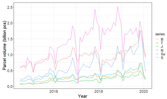 Figure 1. The volume of parcels sent out of the main cities.
 - (2)
- To best centralize capacity and simplify the service procedure during the peak month from 2019 to 2022, Company C usually only keeps one type of service with a fixed discounted price. Therefore, this paper assumes the service quality and price of HSR freight are fixed in the peak month.
- (3)
- This paper assumes that the economy of each city develops independently.
- (4)
- This paper assumes the inspecting train that runs between city B and S has a fixed operating route, capacity, and transport volume during the peak month from 2019 to 2022.
- (5)
- This paper assumes the available number of HSR passenger trains for freight is unchanged during the peak month from 2019 to 2022, and no more than one carriage per train can be used for freight.
- (6)
- This paper assumes it is feasible for all the HSR passenger trains to operate under mixed mode and reserved mode. Since HSR trains cannot stop for enough time at small cities to assemble a large number of parcels, this paper assumes Company C only adopts the reserved mode between main cities.
3.2. Data Collection
The main reason for the lack of empirical analysis of HSR freight is the lack of data of parcels flows transported by HSR between cities, resulting in the inability to validate the model. The flow data in this paper is supported by a railway carrier of China, while other public data are mainly collected from online resources (Table 1).

Table 1.
Variable description and data source.
After cleaning and organizing the HSR freight data, we obtained 84 Origin-Destination (OD) parcel flows transported by B-S HSR between 14 cities and considered their volume as the response variable’s observations. As to selecting candidate factors that may influence the response variable, we considered two aspects: The economic scale and the HSR facility capacity of OD cities.
On the one hand, the OD flow volume is significantly related to the variables that the represent economic and postal scale of OD cities, such as GDP, permanent resident population (POP), the added value of the tertiary industry (AVI), urban retail sales of consumer goods (URG), and the volume of parcels sent out of city (VPC). This paper collects the yearly data of OD cities’ GDP, POP, AVI, and URG from 1998 to 2018, and the monthly data of OD cities’ VPC from 2014/11 to 2020/02. What’s more, we create a new variable, ECO, to represent the city’s economic scale by combining GDP, POP, AVI, and URG. Details are shown in Appendix A.
On the other hand, the facilities of China’s city, such as terminals and rolling stocks, have been the major obstacles for the growth of parcel volume transported by HSR in the short term. We scored the level of all HSR stations from 1 to 4 to indicate the level of fourth, third, second, and first of stations, respectively. Then we sum the scores of all HSR stations of cities to represent terminal accommodation capacity. Besides, the number of daily HSR passenger trains departing from/arriving at 14 cities along B-S HSR at passenger traffic peak have also been collected. We choose the period from February to March to represent the passenger traffic peak because it contains the Spring Festival of China. Most people would go back to work from their hometown when the festival ends, which always produces a rush day to B-S HSR system. It turns out the first workday after the Spring Festival owns the largest number of trains of most cities, and the Thursday three weeks after the festival owns the lowest number. Further, this paper selected the mean value as the variable representing the capacity of HSR train passing cities and selected the difference as the monthly variation of passenger traffic, respectively.
3.3. Forecast Methodology
Generally, the time series forecast method assumes that history is a good reference indicator for judging the future [22]. Thus, the ex-ante forecast usually can be proceeded with time series models based on considering historical data as inputs. However, it is hard to obtain enough HSR freight volume data since the service has only operated for a few years. For such a variable with little historical data, scholars usually forecast it with three steps: First, build a predictive regression model with the variable interested as response variable, which helps explain what causes the variation of it. Second, forecast each predictor with their historical data by time series models. Third, input the results of predictors to the regression model to get the variable’s final forecast result. More details are shown in the graph presented in Figure 2 and the following subsections.
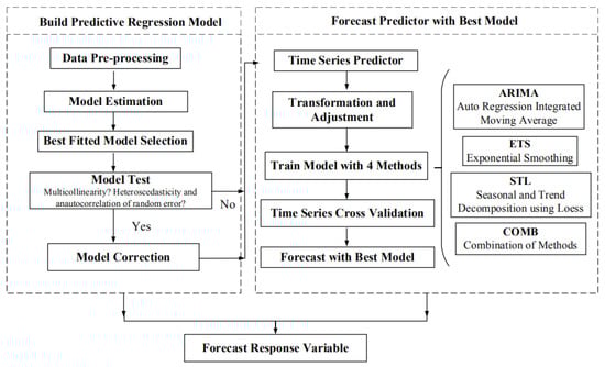
Figure 2.
The flowchart of forecast.
We obtained Figure 2 by compiling the detailed procedure for each stage. At the first stage, the data is sorted and cleaned by R, version 3.6.1, and processed as inputs to build multivariate regression model sets. Then the best model is selected according to the degree of fitness. When fitting the model with data, the paper uses an R package of “leaps” to pick out the best-fitted model set with different sizes from all possible combinations of predictor variables. A few tests would also be applied to check if there is multicollinearity between predictors, heteroscedasticity, and auto-correlation in random error. If there is, the corresponding remedy would be used to correct the model. Once the best predictive regression model is confirmed, stage two will start then. Stage two refers to forecast multiple predictors in the regression. This paper integrates and applies some popular time series methods to train and validate the model to forecast predictors and response variables successively.
3.3.1. Build Predictive Regression Model
This paper’s core regression model is the augmented gravity model, which was first proposed by Tinbergen (1962) to analyze trade relationships between countries empirically. The gravity model’s ability to approximate bilateral trade flows gradually made it one of the most common empirical analysis tools in economics [23]. The purest form of the gravity model is shown as follows:
where represents trade flow from country o to country d, the lowercase letter o and d are short for origin and destination, respectively; G is a regression constant, and stands for the economic dimensions of the country o and d that are being measured. represents the distance between country o and d, is a random error term. The terms are the coefficients to be estimated. Applying the analogy helps acquire the predicted movement of goods between origin and destination. In the original version proposed by Tinbergen (1962), the model is expressed in a log-log form as linear regression, so that parameters are the elasticity of trade flow concerning the predictors. This paper takes the volume of parcels transported from origin city (o) to destination city (d) by HSR as the response variable (), and gets the multivariate linear regression equation:
Here, and denote the economic scale of origin and destination city respectively, and denote the HSR station level in the origin and destination city respectively, represents the mean of HSR passenger trains that depart from the origin city, and represents the mean of HSR passenger trains that arrive at the destination city. indicates the variation of passengers departing from the origin city, indicates the variation of passengers arriving at the destination city. and represent the volume of parcels sent out of the origin and destination city, respectively. indicates the HSR distance between the origin and destination city. is a random error term, is a regression constant, the terms are the coefficients to be estimated.
Especially, and are the combination of four main economic variables including gross domestic product, permanent resident population, the added value of the tertiary industry, and urban retail sales of consumer goods. We reduce the model’s dimension because severe multicollinearity exists between these four variables, and the number of observations smaller than five times the number of variables may lead to unreliable results [24]. The detailed process of reducing dimension is shown in Appendix A.
3.3.2. Forecast Time Series Predictor of Regression Model
Time series forecasting has been widely used for forecasting the trends of economy according to the historical variation. As to forecasting the regression model’s response variable, this paper takes four steps as follows: First, separate the observations of a predictor in one city into two portions, training and test set. Second, apply different time series forecast methods to train the model with training set. Third, make the forecast with the trained model, validate its forecast result with the observations in test set, and then consider the model with minimum difference (forecast error) as the most accurate forecast model. Finally, repeat the three steps mentioned to forecast each economic predictor in each city, then input all the forecast results of predictors to the regression model to get the final forecast result of the response variable.
Many time series methods had been developed during past decades. It is hard to judge which one is the best, since their forecast accuracy varies with the data characteristics. To find out the best forecast model for each predictor in each city, we introduce three classical methods described in Table 2.
Table 2.
Introduction of forecast methods.
Exponential smoothing (ETS) and Auto Regression Integrated Moving Average model (ARIMA) models are the two widely used approaches to time series forecasting and provide complementary approaches to the problem. While ETS models are based on a description of the trend and seasonality in the data, ARIMA models aim to describe the auto-correlations. To best recognize key components of time series (trend and seasonal) and how these enter the exponential smoothing method (e.g., in an additive, damped, or multiplicative manner), we used the extensions of ETS models in Hyndman’s research [27] in this paper. Each consists of a measurement equation that describes the observed data and some state equations that describe how the unobserved components change over time. STL’s (Seasonal and Trend Decomposition using Loess) forecast process usually starts with decomposing out seasonal components and assumes it as unchanged first, then forecasts non-seasonal components with some non-seasonal forecast methods such as ETS and ARIMA.
After applying these methods to train the model with the training set, the best-fitted model set is selected based on identifying the model trained with minimum residual. However, the residual cannot reflect how accurate it can forecast because the forecast accuracy is determined by the error between forecast results of the best-fitted model and the data in the test set. The test set size usually depends on the sample’s length and how far ahead it needs to be forecast. Besides, combining forecast methods sometimes leads to a better forecast accuracy [28]. Thus, this paper developed a combination method using the weighted averages methods mentioned above and set the reciprocal of their accuracy as the weight.
For example, this paper has collected the monthly data of parcels sent from the main cities in the corridor of B-S HSR from July 2014 to February 2020, 68 observations. To forecast the mean volume sent from each city in November 2020, we divide all the cities’ observations into two groups, 59 in training set and 9 in the test set, because the length of the test set should be the same with the steps to forecast (Figure 3). After selecting the best-fitted model of each method, we also need to find the best model with the minimum forecast error from the best-fitted model set. To measure and compare the forecast error of all methods, we adopted one of the most commonly used scale-dependent measures, root mean squared error (RMSE), since it is more effective in dealing with the same scale data that can help us to find the mean of the forecast. An example of selecting the best method to forecast is presented in Table 3.
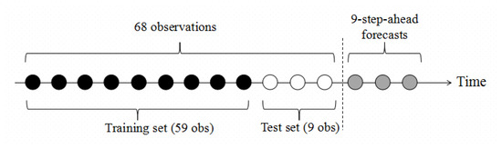
Figure 3.
Time series cross-validation.
Table 3.
Forecast error on forecasting parcel volume sent out of city in November 2020 (million pieces).
Table 3 illustrates the performance error of different methods of forecasting parcel volume sent from cities in November 2020. The number in the cell indicates each method’s error in forecasting the volume of parcels sent out of each city in November 2020. Even under the same forecast step and same variable, the type of best method changes with different cities, and the forecast error of different methods in each row varies greatly. Therefore, to ensure the forecast accuracy to the maximum extent, this paper proceeds every forecast for each variable under each forecast step based on the best method selected under this process.
4. Result and Discussion
4.1. Analysis of Influential Factor on the Flow
Although building the predictive regression model’s primary purpose is to forecast the response variable, the coefficients are statistically significant according to Table A2 in Appendix B, indicating that the correlation between response variable and predictors are reliable. Therefore, the analysis of correlation will be presented in this section. All the coefficients are obtained by fitting the model with the data in 2018, whose description and source can be found in Section 3.2. Under the help of the “leap” package in R software, it is straightforward to fit many predictive models of different sizes with data. However, we need to select the most efficient subset model to achieve the final forecast. The detailed process of model selection can be found in Appendix B. In a word, after the process of training, validating, and selecting, we obtain the final predictive linear regression model presented in Formula (3).
According to Formula (3), the volume of parcels sent from origin city () have made a positive but small impact on the flow volume of parcels transported from origin to the destination city (), which is reasonable since is a small part of . The economic scale of the destination city () also positively impacts , which indicates that the bigger the city’s economic scale is, the more parcels will be shipped to this city through HSR. This may be because people in the cities with a larger economic scale have higher consumption levels and a faster pace of life, which leads to more demand for time-sensitive goods and thus attracts more goods arriving through HSR.
For the mean number of HSR passenger trains departing from origin city (), every 1% increase in its number leads to a 2.23% increase in , which indicates the larger the capacity of HSR passenger trains, the more space to ship parcels through HSR, thus promoting the increase of . Conversely, the variation of passengers departing from origin city negatively impact . This is mainly because China’s railway company always prioritizes passenger transport and only uses the remaining capacity of HSR trains to transport cargoes. If the passenger transport demand increases more than expected at a given time, railway carriers will have to delay or cancel HSR freight service, making the railway carrier appeal to transport fewer parcels from that city if the passengers depart from a city varies a lot.
In general, compared with the value of intercept, all coefficients are small, indicating that the predictors’ influence is relatively weak in a statistical sense. On the one hand, the HSR freight is still in an early stage with a market share lower than 1%, which means the low correlation could be reasonable since the relation between the flow volume and predictors has not yet stabilized or matured. On the other hand, some critical factors may not be included. Currently, the income from transporting HSR freight is still tiny compared with the courier company and railway company’s primary business income. Two of important motivations for their cooperation are courier company strategy investment on HSR transport market and government policy to promote green freight, which is hard to measure and incorporated in the current model. Besides, the low correlation does not affect our model’s good forecast ability, which makes it acceptable, considering the primary purpose of this paper is to forecast. We believe some limitations exist in our method, data, and the results may change as data is collected over a wider area or in a few years, which deserves to explore in the future.
4.2. Analysis of Parcel Flow Volume Forecast
Among all the 84 OD flows that offered service of transporting parcels by HSR, 97.6% of them connected with the 7 main cities (B, T, J, X, N, Su, and S) in November 2018. As HSR freight is still at an early stage of development in China, most of the parcel flows are mainly distributed between large cities. The reason why this situation happens, from the perspective of courier companies, is that they are in urgent need to find faster means of transportation to ship express parcels between big cities and are inclined to delegate the cargoes’ transportation to trucks between small cities. From the perspective of railway companies, HSR passenger trains stop only for a couple of minutes at small city stations in China, making it much more difficult to load and unload large quantities of goods than in big cities. What’s more, the HSR stations’ facilities in big cities also make it easier to coordinate passenger and cargo transportation.
As for the growing trend of these 84 pairs of goods flows in the coming years, although only 17.9% of the parcel flows have a volume over 1 ton in November 2018, and this percentage will reach 84.6% in November 2022. Table 4 shows the top 15 OD pairs with the largest flow volume in November 2018 and forecast volume in November from 2019 to 2022.
Table 4.
Forecast results of top 15 Origin-Destination (OD) flows with largest volume.
According to Table 4, the volume of the parcel between these OD flow varies a lot. Most of the flow volume in 2018 is smaller than 30 tons, but has the potential to exceed it before 2022. Remarkably, the volume of HSR freight between B and S will surpass 100 tons a lot sooner. From the perspective of growth speed, the flow volume between B and J does not change much, but others mostly present the potential to increase 3–10 times from November 2019 to November 2022.
Considering the HSR freight business has just started between many cities in November 2018, it is reasonable to expect the volume to increase dramatically in the next few years. Since courier companies usually delegate very few volumes to the railway company when they start the business in new cities, they will delegate a much larger freight scale after several attempts. For the OD flows that own a volume of over 10 tons in 2018, only those with a distance over 1000 km have the potential to increase a lot, as this is also the most competitive distance range for HSR transport.
4.3. Analysis of Mode Adoption
Currently, there are three modes of HSR freight operating in China, but the inspect mode will not be discussed here due to assumption (4). Based on assumption (5), that the available capacity for freight is fixed during forecast period, and assumption (6), that the reserved mode can only be operated between main cities, this part mainly discusses how to allocate trains under reserved mode and mixed mode in each segment between main cities properly. Generally, a high-speed passenger train (HPT) can carry 240 kg and 6400 kg parcels at maximum under mixed mode and reserved mode, respectively. Additionally, the completion of an HSR freight across multiple cities requires sufficient capacity for each segment of its route. Therefore, to avoid congestion, the operator needs to ensure that each segment’s total capacity is always higher than the volume to a certain extent. Besides, there does exist some HPTs operating under reserved mode in 2018, but if we consider all the HPTs operating HSR freight under mixed mode, the occupancy distribution we get will help us discover which segment tends to saturate without reserved mode.
Figure 4 presents the distribution of capacity and occupancy in two directions, from city B to S (Down) and from city S to B (Up). Each bar with gray and white represents the segment capacity between two cities, which is defined as the total capacity of all the HPTs under mixed mode; the gray bar represents segment occupancy, which is defined as the ratio of the freight volume passing through the segment to the segment capacity. The white bar represents the remaining capacity of each segment.
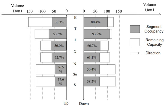
Figure 4.
The distribution of capacity and occupancy under mixed mode in November 2018.
The distribution of capacity at each segment in both directions is similar: The middle segment of J-X and X-J has the minimum capacity around 100 tons; the terminal segment of T-B and Su-S have the largest capacity. The volume transported at all segments ranges from 50 to 110 tons in 2018, and the volume in the down direction is basically larger than those in the up direction, especially for the segment of B-T and T-J. Without adopting reserved mode, most segments’ occupancy in the down direction is larger than 50%, especially for the segment of B-T (80.4%) and T-J (93.2%). Therefore, we suggest the operator give priority to operate HSR passenger trains under reserved mode in the segment of down direction, especially the segment from city B to J.
Due to the result of Section 4.2, the HSR freight volume between most cities are small, but has the potential to increase dramatically in the future. To prevent the growth from being limited by insufficient capacity, this paper suggests Company C operate more HPTs under reserved mode regularly in the future. Based on assumption (5), (6), and the volume forecast result, we offer a solution of mode allocation to ensure each segment’s total capacity equal to the corresponding segment’s volume during the peak month from 2019 to 2022 are shown in Table 5.
Table 5.
The solution of mode allocation of daily trains in peak month from 2019 to 2022.
Looking at Table 5 from left to right, the forecast results during the peak month from 2019 to 2022 show that HSR freight volume at most segments can exceed 200 tons, and the volume in the up direction ranges much more than those in the down direction. The maximum volume in all segments could be 3–7 times larger than in 2018, which is far beyond the capacity of all the HPTs operating only with mixed mode.
Combined with Figure 4 and Table A2, we found the segment occupancy in the up direction is generally lower than that of the down direction in November 2018, but the volume growth in the future is much larger. Therefore, to meet the forecast volume of parcels in the down direction, the operator needs to reserve an average of 4.2 to 8.6 carriages/day to HSR freight transport. For those in the up direction, the average number of carriages/day that need to be reserved could be 2.7 to 13.6. Among all the segments, J-X and X-J are the parts need to reserve most carriages, 5.3~10.1 in down and 4.8~16.3 in up direction, respectively.
There are only two modes discussed in this paper, and we believe that introducing other modes to the operating system will be more interesting. Besides, the forecast period is short due to the limitations of data acquisition. This study also assumes the available capacity is fixed before 2022, and it is worth relaxing such limitations and exploring further analysis closer to reality. The result could also be different if taking the COVID-19 pandemic impact into account, which is beyond this research’s scope, but deserves to be explored in the future.
5. Conclusions
With the fast volume growth of HSR freight in recent years, the remaining freight capacity of high-speed passenger trains under mixed mode running on HSR decreases sharply. Based on the parcel flow forecast analysis and available capacity distribution, we provide a solution for operating trains under reserved mode properly in each segment to relieve the congestion pressure. The main conclusions of this study include the following,
(1) Among all the factors, the city’s economic scale has a positive impact on the city to attract more volume. The number of high-speed trains and the variation range of passenger traffic departs from city have a positive and negative impact on shipping more parcels out of the city, respectively. (2) Among all 84 OD flows in the corridor, the percentage of those volumes over 30 tons increased from 3.6% in 2018 to 26.2% in 2020, and those over 1 ton rose from 17.9% to 84.6%. (3) Among all the B-S HSR corridor segments, T-J should be given priority to operate trains with reserved mode since its segment occupancy is the highest without reserved mode; X-J is the part that deserves to operate the most trains with reserved mode. Our model suggests reserving 5.1–9.8 carriages/day during the peak month from 2019 to 2022. The segment between X and J deserves to reserve the most carriages, 5.3–10.1 carriages/day for J-X, and 4.8–16.3 carriages/day for X-J, respectively.
Author Contributions
The authors confirm contribution to the paper as follows: Conceptualization, H.G., M.Z., and A.G.; methodology, H.G.; software, H.G.; formal analysis, H.G.; investigation, H.G. and M.Z.; writing—original draft preparation, H.G.; writing—review and editing, M.Z. and A.G.; visualization, H.G.; supervision, M.Z. and A.G.; funding acquisition, H.G., M.Z. All authors have read and agreed to the published version of the manuscript.
Funding
This research was supported by the Fundamental Research Funds for the Central Universities (Grant No. 2018YJS062).
Acknowledgments
Hanlin Gao is grateful for the support provided by the China Scholarship Council (No. 201907090002) for a 1-year visiting at the University of Washington (Seattle).
Conflicts of Interest
The authors declare no conflict of interest.
Appendix A. Process of Dimension Reduction
From a statistics perspective, multicollinearity can inflate the estimates’ standard error, thus making it difficult to interpret the sign and the value of regression coefficients [29]. This paper uses the variance inflation factor (VIF) to measure how much a variable contributes to the standard error in the regression, which helps to check multicollinearity in the model. The results are presented in Table A1.
Table A1.
Detecting multicollinearity with variance inflation factors.
Table A1.
Detecting multicollinearity with variance inflation factors.
| VAR | |||||||||
| VIF | 233.6 | 306.6 | 55.2 | 277.9 | 31.1 | 14.4 | 12.5 | 32.0 | 1.2 |
| VAR | |||||||||
| VIF | 210.6 | 488.1 | 59.3 | 306.4 | 13.9 | 9.7 | 10.8 | 57.5 |
o: Origin city; d: Destination city.
Usually, it is acceptable if all VIFs are smaller than 10, but most of the VIFs in the table above are quite large, especially economic variables, which means severe multicollinearity exists in the regression model. Besides, one simple rule of thumb is that the minimum number of observations should be at least five times the number of factors. Compared with 84 observations, 17 variables are too many to get reliable results. Therefore, this paper combines the four main economic variables into new variables based on principal component analysis as follows:
The analysis turns out and explained 96% of the total variance of the corresponding four high-correlated variables, which successfully contains most of their information. The coefficients of Formulas (A1) and (A2) indicate that the four high-correlated variables contribute almost the same to the new variable. We use and to represent the economic scale of origin and destination city in the text.
Appendix B. Process of Selecting the Best Predictive Regression Model
Generally, the biggest challenge to forecast the response variable with a predictive regression model is to select the best model from many candidate models. In this paper, we select the model by stepwise regression method with the help of R software. First, we pass the full model to “step” function, then iteratively add the most contributive predictor and remove any predictors that no longer improve the model fit. Finally, we find the subset of variables in the data set, resulting in the best model based on the criteria of Adj-Rsq. The best subset regressions with different sizes are presented in Table A2.
Table A2.
The best predictive regression model set with different size.
Table A2.
The best predictive regression model set with different size.
| Model1 | Model2 | Model3 | Model4 | Model5 | Model6 | |
|---|---|---|---|---|---|---|
| Intercept | 1.78 ** | −14.72 *** | −28.68 *** | −21.58 *** | −22.54 *** | −21.72 *** |
| 0.83 *** | 1.25 *** | 1.24 *** | 1.23 *** | 1.2 *** | ||
| 0.89 *** | 0.93 *** | 0.93 *** | 0.90 *** | 0.89 *** | ||
| 0.82 *** | ||||||
| 0.71 * | 2.23 ** | 2.22 *** | 2.14 *** | |||
| −1.70 *** | −1.71 ** | −1.79 ** | ||||
| 0.27 | 0.24 | |||||
| 0.24 | ||||||
| 0.13 | 0.47 | 0.51 | 0.52 | 0.52 | 0.52 | |
| BP Test (p-value) | 0.00 | 0.20 | 0.69 | 0.44 | 0.84 | 0.59 |
| BG Test (p-value) | 0.00 | 0.61 | 0.31 | 0.31 | 0.29 | 0.20 |
.
Heteroscedasticity and autocorrelation usually lead to an inefficient and unstable regression model, which can later yield bizarre predictions. To ensure the reliability of model results, we used Breusch–Pagn (BP) test and Breusch–Godfrey (BG) test to check whether there exist heteroscedasticity and autocorrelation in residuals. The bottom two rows of Table A2 show that all p-values of tests are larger than 0.05, which indicates a failure to reject that the variance of residuals is constant, and there is no serial autocorrelation of any order. Thus, there is no heteroscedasticity or autocorrelation in these models.
According to Table A2, compared with other models listed in the table, model 4 has the least predictors with the highest (0.52), indicating the best ability and efficiency to fit model and forecast the response variable. Although the of model 5 and 6 are 0.52 too, keeping variables that are not statistically significant can reduce the model’s precision. Therefore, this paper decides to adopt Model 4 to forecast parcel volume between cities in the B-S HSR corridor.
References
- Zhao, J.; Zhao, Y.; Li, Y. The variation in the value of travel-time savings and the dilemma of high-speed rail in china. Transp. Res. Part A Policy Pract. 2015, 82, 130–140. [Google Scholar] [CrossRef]
- Behiri, W.; Belmokhtar-Berraf, S.; Chu, C. Urban freight transport using passenger rail network: Scientific issues and quantitative analysis. Transp. Res. Part E 2018, 115, 227–245. [Google Scholar] [CrossRef]
- Kikuta, J.; Tatsuhide, I.; Izuru, T.; Shu, Y.; Tadashi, Y. New Subway-Integrated City Logistics Szystem. Procedia Soc. Behav. Sci. 2012, 476–489. [Google Scholar] [CrossRef]
- Regue, R.; Abigail, L.B. Appraising Freight Tram Schemes: A Case Study of Barcelona. Eur. J. Transp. Infrastruct. Res. 2013, 13, 56–78. [Google Scholar]
- Rowangould, G. Public financing of private rail infrastructure to reduce highway congestion: A case study of public policy and decision making in the United States. Transp. Res. Part A 2013, 57, 25–36. [Google Scholar] [CrossRef]
- Rotem-Mindali, O.; Salomon, I. The impacts of e-retail on the choice of shopping trips and delivery: Some preliminary findings. Transp. Res. A 2007, 41, 176–189. [Google Scholar] [CrossRef]
- Pazour, J.A.; Meller, R.D.; Pohl, L.M. A model to design a national high-speed rail network for freight distribution. Transp. Res. Part A 2010, 44, 119–135. [Google Scholar] [CrossRef]
- Jeong, S.J.; Lee, C.G.; Bookbinder, J.H. The European freight railway system as a hub-and-spoke network. Transp. Res. Part A Policy Pr. 2007, 41, 523–536. [Google Scholar] [CrossRef]
- Gao, H.; Zhang, M.; Zhang, Y. Exploring the alternative modes of eco-friendly express freight transport. Appl. Ecol. Environ. Res. 2019, 17, 8805–8816. [Google Scholar] [CrossRef]
- Ohnell, S.; Woxenius, J. An industry analysis of express freight from a European railway perspective. Int. J. Phys. Distrib. Logist. Manag. 2003, 33, 735–751. [Google Scholar] [CrossRef]
- Troche, G. Activity-Based Rail Freight Costing a Model for Calculating Transport Costs in Different Production Systems. Ph.D. Thesis, KTH Royal Institute of Technology, Stockholm, Sweden, 2009. [Google Scholar]
- Ertem, M.A.; Keskin, Z.M. Freight transportation using high-speed train systems. Transp. Lett. 2016, 8, 250–258. [Google Scholar] [CrossRef]
- Mathieu, S. High-speed rail for freight: Potential developments and impacts on urban dynamics. Open Transp. J. 2016, 10, 57–66. [Google Scholar]
- Tan, K.; Zhang, C. Research on high speed railway freight mode in France. Chin. Railw. 2014, 3, 16–20. [Google Scholar]
- Cochrane, K.; Saxe, S.; Roorda, M.J.; Shalaby, A. Moving freight on public transit: Best practices, challenges, and opportunities. Int. J. Sustain. Transp. 2017, 11, 120–132. [Google Scholar] [CrossRef]
- Watson, I.; Ali, A.; Bayyatia, A. Freight transport using high-speed railways. Int. J. Transp. Dev. Integr. 2019, 3, 103–116. [Google Scholar] [CrossRef]
- Bi, M.K.; He, S.W.; Xu, W. Express delivery with high-speed railway: Definitely feasible or just a publicity stunt. Transp. Res. Part A Policy Pr. 2019, 120, 165–187. [Google Scholar] [CrossRef]
- Liang, X.H.; Tan, K.H. Market potential and approaches of parcels and mail by high speed rail in China. Case Stud. Transp. Policy 2019, 7, 583–597. [Google Scholar] [CrossRef]
- Yu, X.; Lang, M.; Gao, Y.; Wang, K.; Su, C.-H.; Tsai, S.-B.; Huo, M.; Yu, X.; Li, S. An Empirical Study on the Design of China High-Speed Rail Express Train Operation Plan—From a Sustainable Transport Perspective. Sustainability 2018, 10, 2478. [Google Scholar] [CrossRef]
- Liang, X.H.; Tan, K.H.; Whiteing, A.; Nash, C.; Johnson, D. Parcels and mail by high speed rail-A comparative analysis of Germany, France and China. J. Rail Transp. Plan. Manag. 2016, 6, 77–88. [Google Scholar] [CrossRef]
- Douglas, C.; Cheryl, L.; Murat, K. Introduction to Time Series Analysis and Forecasting, 2nd ed.; Wiley: Hoboken, NJ, USA, 2008; pp. 365–369. [Google Scholar]
- Hyndman, R.; Athanasopoulos, G. Forecasting: Principles and Practice 2013. Available online: http://otexts.org/fpp/ (accessed on 17 October 2013).
- Keith, H.; Thierry, M. Gravity Equations: Workhorse, Toolkit, and Cookbook 2013. Available online: https://hal-sciencespo.archives-ouvertes.fr/hal-00973067 (accessed on 27 September 2013).
- Hair, J.F., Jr.; Anderson, R.E.; Tatham, R.L.; Black, W.C. Multivariate Data Analysis, 3rd ed.; Prentice Hall: Englewood Cliffs, NJ, USA, 2010. [Google Scholar]
- Winters, P.R. Forecasting sales by exponentially weighted moving averages. Manag. Sci. 1960, 6, 324–342. [Google Scholar] [CrossRef]
- Cleveland, R.B.; Cleveland, W.S.; McRae, J.E.; Terpenning, I.J. STL: A seasonal-trend decomposition procedure based on loess. J. Off. Stat. 1990, 6, 3–33. [Google Scholar]
- Hyndman, R.J.; Koehler, A.B.; Ord, J.K.; Snyder, R.D. Forecasting with Exponential Smoothing: The State Space Approach; Springer Science & Business Media: Berlin, Germany, 2008. [Google Scholar]
- Clemen, R. Combining forecasts: A review and annotated bibliography with discussion. Int. J. Forecast. 1989, 5, 559–608. [Google Scholar] [CrossRef]
- Bruce, P.; Andrew, B. Chp4: Regression and Prediction. Practical Statistics for Data Scientists; Shannon Cutt, O’Reilly Media: Sebastopol, CA, USA, 2017; pp. 190–195. [Google Scholar]


Publisher’s Note: MDPI stays neutral with regard to jurisdictional claims in published maps and institutional affiliations. |
© 2020 by the authors. Licensee MDPI, Basel, Switzerland. This article is an open access article distributed under the terms and conditions of the Creative Commons Attribution (CC BY) license (http://creativecommons.org/licenses/by/4.0/).