Abstract
This paper investigates the nonlinear relationship between CO2 emission and economic development using a newly developed functional coefficient panel model. In contrast to the existing literature, which suggests that the income elasticity of CO2 emission is parametrically modeled as a function of income, the income coefficient of CO2 emission is set as a function of both income and time. Then, we estimate the income elasticity in a nonparametric way using the country panel data covering 1971–2017. By doing so, we impose richer dynamics to the income elasticity not only over income but also over time. Our empirical results indicate that the income elasticity has decreased over time for high-income countries, whereas it has increased over time for low-income countries.
1. Introduction
It is difficult to understand how the environmental quality and economic growth affect the standard of living of a country. As the economy begins to grow, people are likely to use more environmental resources, giving them a better quality of life with the cost of environmental degradation. Once the economy reaches out to the industrially matured state, however, environmental degradation begins to deteriorate the quality of life, causing people to give more value to environmental quality over economic growth. This economic story depicts the inverted-U-shaped relationship between environmental degradation and per capita income in either a cross-section, time series, or panel data framework [1,2]. This empirical phenomenon is known as the Environmental Kuznets Curve.
Since Grossman and Krueger [3], who provided the empirical evidence for the inverted-U shaped relationship, a large number of studies have investigated its nonlinearity with various econometric methodologies. The typical approach is to model the income elasticity of the environmental pollutants, such as carbon dioxide and sulfur dioxide emissions, as a function of income. By allowing the income elasticity to change over the income itself, the researcher has attempted to derive its nonlinearity over income. Note that the change in utility, technology, or sectoral shift of the economy, which can be proxied by the time factor, can also affect the environmental quality in a different way. In such a context, several authors attribute the inverted-U-shaped relationship to the sectoral share of the clean service economy and increased preference on environmental quality [1,4,5].
Moreover, there is growing literature on China’s decoupling relationship as China becomes the world’s largest CO2 emitter. Beginning with Yu et al. [6], who study the relationship between carbon dioxide emission and economic development using the feasible GLS method in the panel data framework. On the other hand, Bloch et al. [7] employ the cointegration and error correction model to show how coal consumption and income are correlated both supply and demand side. Xie et al. [8] identify the determinants of power industrial CO2 emission with the autoregressive distributed lag model, showing that improved coal-fired power generation efficiency and decreasing terminal energy intensity reduce the decoupling index.
Note that the international agreement on climate change such as Kyoto Protocol and Paris Agreement goes beyond the mitigation strategy of the impact of climate change. It prompts each country to plan a new economic growth strategy, technology diffusion, and energy system, in order to reduce greenhouse gas emissions [9,10]. Specifically, the advance in renewable energy technology and the improvement in energy efficiency have been playing a role in reducing greenhouse gas emission, not only for developed countries, but also for developing countries. These technological factors would be different with the economic growth factor. In this light, the income elasticity would be misdirected if we assume that it is only a function of economic growth. Throughout this paper, we address the research question that the income elasticity can be a function of both economic growth and time factor. By doing so, we can identify the net effect of economic growth over different income levels and time.
This paper relates to the literature that studies econometric modeling for the environmental Kuznets curve. In the literature, specifically, most of the empirical studies have focused on the nonlinearity between CO2 emission and economic development by utilizing the quadratic linear regression model, as given by
Here, is log of CO2 emission per capita of country at time , and , are the log of GDP per capita and the log squared GDP per capita, respectively. Note that the positive and the negative provide the evidence of the environmental Kuznets curve.
Since environmental pollutant emission and income variables are known to have a stochastic trend in their sample path, the linear cointegration technique has been routinely exploited for estimating the quadratic linear regression (1). Although the regression model (1) looks simple, there is an important econometric issue that the squared transformation of the integrated process is not an integrated process at any order. This implies that the regression Equation (1) cannot represent the cointegrating relationship. Consequently, the standard linear cointegration technique would be invalid for the quadratic regression of the environmental Kuznets curve.
To overcome such an econometric problem, Wagner and Hong [11] propose the cointegrating polynomial regression, which includes integer power of unit root process as a regressor. Since the integer power of the integrated process has a different asymptotic order with the original integrated process, a new asymptotic theory would be needed for statistical inference. They developed the fully modified Least Squares (LS) method in this framework, and derived the corresponding Kwiatkowski–Phillips–Schmidt–Shin (KPSS)-type cointegration test. Using their econometric approach, Wagner [2] finds less evidence for the environmental Kuznets curve hypothesis, compared to the empirical findings provided in the existing literature.
Another stream of literature considers a nonparametric estimation technique in testing the environmental Kuznets curve hypothesis. Millimet et al. [12] and Bertinelli & Strobl [13] exploit the local constant estimator with the partially linear model, although they do not consider the nonstationarity of GDP in constructing the nonparametric kernel-based regression estimator. Note that Phillips & Park [14] show that the convergence rate of kernel-type regression estimator for unit root process is slower than that for stationary process. Other nonparametric methods, such as spline interpolation [15] have a similar problem.
The contribution of this paper can be summarized as follows. We apply a novel nonparametric panel estimation technique of Chang et al. [16] to investigate the nonlinear relationship between CO2 emission and economic growth. To the best of our knowledge, our study is the first attempt to estimate the long-run relationship between CO2 emission and economic development using a functional coefficient panel methodology. We set the income coefficient to be a function of both time and the regressor itself, but our target is carbon dioxide emissions. By doing so, we can identify the income response to the carbon dioxide emission across income and time.
It is worth emphasizing that only a few studies consider the income elasticity as a function of time for testing the environmental Kuznets curve hypothesis. Since the income elasticity solely depends on its income level, we cannot separate its temporal change from the income-dependent coefficient function. Notably, Mikayilov et al. [17] apply the time-varying coefficient methodology of Park and Hahn [18] for the environmental Kuznets curve to model the time-varying income elasticity. Nevertheless, even though they allow for a more flexible functional form, it does not account for the impact of change at the different income level.
2. Data
The data used in our analysis consist of the balanced panel of 100 countries covering the period of 1971–2017. The real GDP per capita at chained purchasing power parity (in 2011 million dollars) are drawn from the Penn World Table 9.1. (downloaded from https://www.rug.nl/ggdc/productivity/pwt on 24 February 2020). The CO2 emission data (in million metric tons) are obtained from OECD Air and GHG emission dataset (downloaded from https://data.oecd.org/air/air-and-ghg-emissions.htm on 24 February 2020), and are converted to per capita term using the population (in millions) variable of PWT 9.1. Although we can extract 136 countries from the original dataset, 100 countries were used in our analysis. Specifically, we exclude 32 countries (most of these are former Soviet bloc countries) because of missing CO2 or GDP observations, and then additionally, four countries (United Arab Emirates, Qatar, Kuwait, and Brunei) are omitted because of the unreliability of the GDP data.
To obtain a more reliable estimate, Chang et al. [16] propose the statistical method for grouping the individual country’s variable. They first categorize the individual country’s GDP into ten groups by designed quantiles (we use the same quantile as used in Table 1 of Chang et al. [16]), and then their CO2 emission and GDP variables are weighted averaged by corresponding GDP ratio for each group. As in Chang et al. [16], moreover, we create CO2 per capita index (2000 = 100), in order to get rid of cross-country heterogeneity in the original variable. This paper strictly follows the way of Chang et al. [16], in order to generate the grouped variable. Finally, our final dataset consists of 10 groups over 47 years for each CO2 emission and GDP dataset. Figure 1 illustrates the generated grouped variables.

Table 1.
Unit root test results for CO2 emission and GDP with constant and time trend terms included in the unit root equation. The optimal lag lengths for the ADF test are chosen by BIC and presented in parentheses. ***, **, and * represent statistical significance at 1%, 5%, and 10%, respectively.
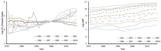
Figure 1.
Logs of CO2 emission per capita index and GDP per capita.
3. Econometric Model and Methodology
In this paper, we apply the functional-coefficient panel methodology of Chang et al. [16], instead of including the squared GDP per capita in the model. By doing so, we allow the coefficient of GDP per capita to vary over time and GDP per capita itself. The functional-coefficient panel model of Chang et al. [16] is given by
where is log of CO2 emission per capita of country at time , and is the log of GDP per capita, and is the group binaries for cross-sectional heterogeneity. Note that the income elasticity, is now modeled as a function of time and GDP per capita, . Here, we assume the stationarity of , but nonstationarity of
We may consider the equation as the semiparametric panel cointegration model, in the sense that the first term is modeled in a parametric sense and the functional-coefficient, is estimated by the nonparametric way. It is worth noting that the functional-coefficient panel methodology of Chang et al. [16] is an income-extended version of the time-varying coefficient methodology of [18].
In what follows, we follow the two-step estimation procedure of [16]. Specifically, the equation is rearranged as given by
Here, the time is re-denoted as at the first argument of in order to avoid the notational confusion. Assuming that the estimator is known, we can estimate the income coefficient by
Here, is the weight function at country and time . Note that can be estimated by the nonparametric regression of on respectively, as given by
Consequently, the consistent estimator of the parameter, can be provided by the least-squares regression of
As a result, the income coefficient, which is the parameter of interest, is calculated as
Note that the weight function, is estimated by
where K is the usual kernel function, which defines weights at time and log GDP per capita, and are the bandwidths for time and log GDP per capita. The formal procedure of the bandwidth selection for the nonstationary cointegrating regression, such as ours, has not been developed, although some theory for the stationary regression has been studied.
Notwithstanding, Phillips & Park [14] provide some asymptotic background on the kernel regression estimators of the nonstationary regression. They show that the limit distribution of the kernel estimator is mixed normal for nonstationary unit-root case, and its convergence rate is slower than the kernel estimator for stationary case, because the nonstationary regression involves unstable and volatile observations. This implies that there is a reasonable direction for choosing the bandwidths, although we do not have a formal theory for our nonstationary regression.
Once we estimate the income coefficient, we can estimate the income elasticity of the individual country. The income elasticity, which is defined as the partial derivative of CO2 emission per capita with respect to the GDP per capita, is calculated as
for any time and income . Note that is the partial derivative of with respect to the second argument , implying that the income elasticity itself is varying over unless y is zero. Practically, the partial derivative, can be calculated as
with 0.01.
4. Estimation Results
As we mentioned before, our model represents the cointegrating relationship between CO2 emission and real GDP. As a pre-step, we examine the nonstationarity of CO2 emission and GDP. To do so, we employ both the Augmented Dickey–Fuller (ADF) unit-root test and the Kwiatkowski–Phillips–Schmidt–Shin (KPSS) stationarity test. In both tests, we include constant and time trend terms in unit root equation. Note that the null hypothesis of the ADF test is that there is a unit root in the series, whereas the KPSS test assumes the null of stationarity in the series. The optimal lag length in the ADF test is chosen by the Schwarz/Bayesian information criterion (BIC) from a maximum of 10.
Table 1 provides the unit root test results. The test results show that most of the grouped variables have a unit root, indicating the integrated process of order one. Although there are some cases that one of the tests rejects the nonstationarity, their p-values are not decisive. Moreover, no series provides the rejection results of both tests.
In what follows, we employ the two-step estimation procedure of [16]. In the first step, we estimate the group fixed effect of the parametric part using the partially linear estimation procedure, which is tabulated in Table 2. Note that the standard asymptotic theory cannot be applied due to the nonstationarity of the variable. Therefore, the asymptotic standard error in Table 2 is calculated by the bootstrapping method. Noticeably, the fixed effect terms from group 7 to group 10 turn out to be statistically significant, implying that the reduction in variance by exploiting larger samples enables us to measure the fixed effect terms in a precise way.
Table 2.
First-step fixed effect estimation results for grouped variables.
Nonparametric technique is invited to estimate the income coefficient, and therefore searching procedure for optimal bandwidth size is required. With bigger bandwidth size than the optimal, the income coefficient would be over-smoothed, making us overlook a high-frequency relationship. With smaller bandwidth size, on the other hand, the estimated income coefficient would be noisy, masking the important long-run relationship by the short-run noisy components. Following the recommendation of [16] for nonstationary data, we estimate the bias-corrected AIC procedure and the cross-validation method, and take five times the bigger one. We also adapted the interrelated two-dimensional bandwidth selection, giving us values, 0.1343 for time, 0.0484 for income.
Figure 2 provides the estimated income coefficient when the GDP per capita is ranged from USD 400 to USD 60,000 (6 to 11 in log). The existing literature assumes that the income elasticity varies over either time or income itself. As illustrated in Figure 2, however, this paper allows the income elasticity to change over both time and income itself. Specifically, Figure 2 provides the estimated income coefficient using ten different income groups, of which each group’s income is calculated as the weighted average of GDP per capita of the members.
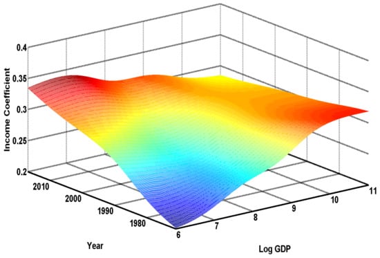
Figure 2.
Estimated income coefficient for grouped variables.
Figure 3 provides a two-dimensional representation of Figure 2 with fixed years and income levels. The income coefficients with the fixed years of 1975, 1985, and 1995, slowly increase over the income, and then become flatter at the high-income level. In the meantime, when the fixed year is 2015, the income coefficients slowly decrease over the income, and then become flatter. This result implies that, while the income coefficient of countries with high incomes has been higher, the opposite phenomenon has been observed in the last decade. The manufacturing-intensive countries would generate more CO2 emissions as they became richer, but the service-intensive countries would reduce the environmental pollutants in the early stages of growth. Once both manufacturing- and service-intensive countries reach a certain high-income level (USD 20,000), the income responses become insensitive to the income.
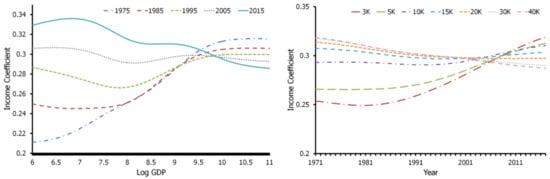
Figure 3.
Estimated income coefficients at the selected year (left) and income level (right).
Looking at the income coefficient of the right panel of Figure 3, the income coefficients of low-income countries are slowly increasing over time, meaning that the sectoral shift or technological advancement of those countries by the process of dematerialization would occur. However, the income coefficients of the developed countries have not been changed or have instead decreased for the entire sample period.
It is important to note that the estimation results of Figure 3 prove the validity of the environmental Kuznets curve hypothesis in a two-dimensional way: time and income. Previous studies examine the inverted-U-shaped relationship between environmental degradation and per capita income without or just partially considering time-varying components, such as the technology renovation over time. However, the spillover of technologies that can reduce greenhouse gases over time can be critical to change the relationship between past greenhouse gas emissions and economic growth. In that sense, we control time-varying components that can affect the relationship by employing the functional coefficient with multiple arguments (time and GDP). In a time dimension, the income coefficient steadily grows over time for low-income country, and is stable for middle-income country, and decreases over time for high-income country. In an income dimension, the income coefficient grows over income in the past, but decreases over income in the present. Combining these two-dimensional inverted U-shapes would provide more comprehensive understanding of the classical environmental Kuznets curve hypothesis by segregating the effect of sectoral shift from the income effect.
Looking at the income elasticities of the grouped variables and selected countries of Figure 4, the temporal patterns of the income elasticities are clearly described. It is worth noting that the absolute level of the income elasticity would not provide a meaningful interpretation, in the sense that there might be omitted variable bias in the fixed effect terms. Note that Neagu [19] has considered an economic complexity index as an additional covariate. Instead, we may give an economic interpretation on the estimated income elasticity as the relative magnitude of the income effect on CO2 emission, and therefore, temporal dynamics is the key to understanding the graphs of Figure 4 [20].
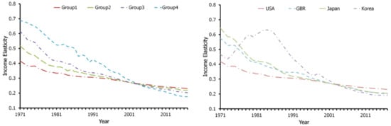
Figure 4.
Estimated income elasticities for each group (left) and selective countries (right).
As an example, Group 1’s income elasticity of the left panel of Figure 4 was 0.38 in 1975, and was 0.24 in 2015, making the difference in the income elasticity −0.14 for forty years. Since all the variables in the model are in the log, we can provide an interpretation that CO2 emission has been decreased by 0.14, or 14% when Group 1’s GDP increases by about 110% for that period (USD 25,924 in 1975 to USD 54,456 in 2015). As such, the slope of income elasticity of Group 4 is much steeper than that of Group 1, which means that the size of reduction in CO2 emission of the low-income country has been much greater than that of high-income country.
The right panel of Figure 4 illustrates the income elasticities of the selective countries, the United States, Great Britain (GBR, hereafter), Japan, and Korea. As expected, the income elasticities of the United States, GBR, and Japan have been steadily decreasing over time, and not surprisingly, Japan’s slope is steeper than slopes of GBR and the United States. Notably, the income elasticity of Republic of Korea appears to have an inverted U-shape, of which their peak is located around the year of 1985. The response to CO2 emission of Republic of Korea would show a similar shape with that to electricity consumption described in Chang et al. [16], implying that the sectoral shift from manufacturing to service industry had occurred.
Even taking account of the possible bias of the estimated income elasticity, it is worth noting that the income elasticities for all countries are positive and less than unity for our sample period (1971–2017). According to the conventional definition of the environmental Kuznets curve, the income elasticity changes sign from positive to negative when the income reaches a threshold level. Thus, our result does not support the EKC hypothesis. Our results, however, are consistent with the well-known phenomenon of relative decoupling between CO2 emission and economic growth. Mikayilov et al. [17] report the relative decoupling phenomenon of most countries, and some of the elasticities greater than unity. We believe that this apparent economic phenomenon could be statistically realized by the functional-coefficient panel methodology, which allows the income elasticity to change over time and income itself.
5. Conclusions
This study employs a novel nonparametric panel estimation approach recently proposed by Chang et al. [16] to estimate the nonlinear relationship between income and CO2 emission. To the best of our knowledge, our study is the first to attempt to use panel functional coefficient model in estimating the long-run relationship between CO2 emission and economic growth. The coefficient is set as a function of both time and the regressor itself, typically GDP per capita in our context. The main advantage of our functional coefficient approach is two-fold. First, our methodology does not need a squared GDP, thus we do not have any econometrical problem induced by nonstationary variables. Instead, we use functional coefficients technique to allow for more flexible model specifications. Second, our model distinguishes whether the variation in elasticity comes from a change in time or income level. Therefore, we can conduct counterfactual analysis, which describes one variable with another variable fixed.
Our empirical results are generally consistent with findings reported in literature that income elasticities for most of developed countries have decreased over time, while developing countries such as South Korea have the inverted U-shape of income elasticity. In addition, the slope of income elasticity of the middle-income group is much steeper than high income group country. This result can be interpreted that the industrial structure is fixed in high-income countries, which means that there is no longer a sharp decrease in CO2 emissions as income increase, whereas relatively steep decreases in middle-income countries are caused by sectoral shift such as toward service intensive industrial structure.
From a policy point of view, this has meaningful implications. Under the business as usual (BAU) scenario, we cannot avoid a global catastrophe from climate change. The highly developed countries still account for a large portion of global emissions. Therefore, CO2 emissions will not decrease even if the economy grows sufficiently. This implies that CO2 emissions cannot meet the 2 °C or 1.5 °C Paris Agreement goal without innovative and drastic mitigation efforts. Although this paper employs the newly developed functional coefficient panel model to test the environmental Kuznets curve hypothesis, the model can also be used to forecast CO2 emission, which is important information for policymakers to achieve sustainable economic growth. We leave these tasks for our future research.
Author Contributions
K.N., S.L. and H.J. equally contributed to the conception of the research, programming, statistical estimation, checking, and proofreading. K.N. and H.J. wrote the paper, S.L. curated the data, and H.J. responded to the editor and referees. All authors have read and agreed to the published version of the manuscript.
Funding
This work was conducted by the Korea Environment Institute (2020-090) with the Korea Energy Agency’s support.
Conflicts of Interest
The authors declare no conflict of interest.
References
- Dinda, S. Environmental Kuznets Curve Hypothesis: A Survey. Ecol. Econ. 2004, 49, 431–455. [Google Scholar] [CrossRef]
- Wagner, M. The Environmental Kuznets Curve, Cointegration and Nonlinearity. J. Appl. Econ. 2015, 30, 948–967. [Google Scholar] [CrossRef]
- Grossman, G.M.; Krueger, A.B. Economic Growth and the Environment. Q. J. Econ. 1995, 110, 353–377. [Google Scholar] [CrossRef]
- Arrow, K.; Bolin, B.; Costanza, R.; Dasgupta, P.; Folke, C.; Holling, C.; Jansson, B.-O.; Levin, S.; Mäler, K.-G.; Perrings, C.; et al. Economic growth, carrying capacity, and the environment. Environ. Dev. Econ. 1996, 1, 104–110. [Google Scholar] [CrossRef]
- Carson, R.T.; Jeon, Y.; McCubbin, D.R. The relationship between air pollution emissions and income: US Data. Environ. Dev. Econ. 1997, 2, 433–450. [Google Scholar] [CrossRef]
- Yu, Y.H.; Zheng, X.Y.; Zhang, L. Carbon dioxide emission and economic development: A panel data analysis. Econ. Theory Bus. Manag. 2011, 3, 72–81. [Google Scholar]
- Bloch, H.; Rafiq, S.; Salim, R.A. Coal consumption, CO2 emission and economic growth in China: Empirical evidence and policy responses. Energy Econ. 2012, 34, 518–528. [Google Scholar] [CrossRef]
- Xie, P.; Yang, F.; Mu, Z.; Gao, S. Influencing factors of the decoupling relationship between CO2 emission and economic development in China’s power industry. Energy 2020, 209, 118341. [Google Scholar] [CrossRef]
- Miyamoto, M.; Takeuchi, K. Climate agreement and technology diffusion: Impact of the Kyoto Protocol on international patent applications for renewable energy technologies. Energy Policy 2019, 129, 1331–1338. [Google Scholar] [CrossRef]
- Vrontisi, Z.; Fragkiadakis, K.; Kannavou, M.; Capros, P. Energy system transition and macroeconomic impacts of a European decarbonization action towards a below 2 °C climate stabilization. Clim. Chang. 2020, 162, 1857–1875. [Google Scholar] [CrossRef]
- Wagner, M.; Hong, S.H. Cointegrating polynomial regressions: Fully modified ols estimation and inference. Econ. Theory 2016, 32, 1289–1315. [Google Scholar] [CrossRef]
- Millimet, D.L.; List, J.A.; Stengos, T. The Environmental Kuznets Curve: Real Progress or Misspecified Models? Rev. Econ. Stat. 2003, 85, 1038–1047. [Google Scholar] [CrossRef]
- Bertinelli, L.; Strobl, E. The environmental Kuznets curve semi-parametrically revisited. Econ. Lett. 2005, 88, 350–357. [Google Scholar] [CrossRef]
- Phillips, P.C.; Park, J.Y. Nonstationary Density Estimation and Kernel Autoregression. Cowles Found. Dis. Paper, No. 1181. 1998. Available online: https://ideas.repec.org/p/cwl/cwldpp/1181.html (accessed on 7 December 2020).
- Schmalensee, R.; Stoker, T.M.; Judson, R.A. World carbon dioxide emissions: 1950–2050. Rev. Econ. Stat. 1998, 80, 15–27. [Google Scholar] [CrossRef]
- Chang, Y.; Choi, Y.; Kim, C.S.; Miller, J.I.; Park, J.Y. Disentangling temporal patterns in elasticities: A functional coefficient panel analysis of electricity demand. Energy Econ. 2016, 60, 232–243. [Google Scholar] [CrossRef]
- Mikayilov, J.I.; Hasanov, F.J.; Galeotti, M. Decoupling of CO2 emissions and GDP: A time-varying cointegration approach. Ecol. Indic. 2018, 95, 615–628. [Google Scholar] [CrossRef]
- Park, J.Y.; Hahn, S.B. Cointegrating regressions with time varying coefficients. Econ. Theory 1999, 15, 664–703. [Google Scholar] [CrossRef]
- Neagu, O. The Link between Economic Complexity and Carbon Emissions in the European Union Countries: A Model Based on the Environmental Kuznets Curve (EKC) Approach. Sustainability 2019, 11, 4753. [Google Scholar] [CrossRef]
- Chang, Y.; Kim, C.S.; Miller, J.I.; Park, J.Y.; Park, S. Time-varying Long-run Income and Output Elasticities of Electricity Demand with an Application to Korea. Energy Econ. 2014, 46, 334–347. [Google Scholar] [CrossRef]


Publisher’s Note: MDPI stays neutral with regard to jurisdictional claims in published maps and institutional affiliations. |
© 2020 by the authors. Licensee MDPI, Basel, Switzerland. This article is an open access article distributed under the terms and conditions of the Creative Commons Attribution (CC BY) license (http://creativecommons.org/licenses/by/4.0/).