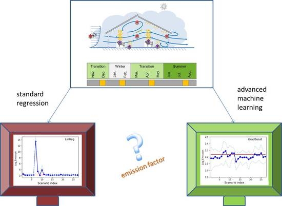
How the Selection of Training Data and Modeling Approach Affects the Estimation of Ammonia Emissions from a Naturally Ventilated Dairy Barn—Classical Statistics versus Machine Learning

Abstract

Environmental protection efforts can only be effective in the long term with a reliable quantification of pollutant gas emissions as a first step to mitigation. Measurement and analysis strategies must permit the accurate extrapolation of emission values. We systematically analyzed the added value of applying modern machine learning methods in the process of monitoring emissions from naturally ventilated livestock buildings to the atmosphere. We considered almost 40 weeks of hourly emission values from a naturally ventilated dairy cattle barn in Northern Germany. We compared model predictions using 27 different scenarios of temporal sampling, multiple measures of model accuracy, and eight different regression approaches. The error of the predicted emission values with the tested measurement protocols was, on average, well below 20%. The sensitivity of the prediction to the selected training dataset was worse for the ordinary multilinear regression. Gradient boosting and random forests provided the most accurate and robust emission value predictions, accompanied by the second-smallest model errors. Most of the highly ranked scenarios involved six measurement periods, while the scenario with the best overall performance was: One measurement period in summer and three in the transition periods, each lasting for 14 days.

1. Introduction

National and international directives, such as the EU-28 National Emission Ceilings (NEC, see https://www.eea.europa.eu, last access 16 December, 2019), urge for a substantial reduction of airborne pollutants in order to limit climate change and protect the environment and human health [1,2]. The evaluation of emission reduction measures requires a reliable quantification of pollutant gas emissions in all economic sectors, including agriculture. Ammonia is, besides greenhouse gases and particulate matter, one of the most crucial substances to monitor [3,4,5]. It contributes to the formation of secondary particulate matter and leads to acidification and eutrophication of soil and water. It thereby indirectly contributes to the earth’s radiation budget by affecting aerosol formation and plant coverage.

Agriculture contributes around 92% to the European ammonia emissions [6]. Livestock housing, particularly the management of slurry and manure, is the main source of ammonia emissions from agriculture [7]. The evaluation of housing systems’ emissions is, however, challenging and involves large uncertainties. The common emission standard uncertainty is at least 10%, and it can be considerably higher if natural ventilation of animal buildings is involved [8].

In order to effectively mitigate emissions, first, a measurement and analysis strategy that permits the accurate extrapolation of annual emission values is needed. As dairy cattle are mostly housed in naturally ventilated buildings, are highly economically relevant, and their housing contributes to around 10% of the total ammonia emissions from livestock, in the present study, we focus on ammonia emissions from this husbandry system.

In naturally ventilated dairy buildings, air exchange rates and gaseous emissions are usually measured by indirect gas-balancing methods on a few days distributed over the year (including hot, cold, and moderate days). Data from those measurements are later extrapolated to annual emission values using statistical methods [9,10,11]. Intermittent measurements are common in order to reduce the high cost of continuous ammonia emission measurements, since the expensive equipment can be used in several buildings for short periods [12]. For dairy cattle husbandry, an international expert group recently formulated recommendations for temporal sampling to ensure a minimum standard (cf. www.vera-verification.eu, last access 4 December, 2019). The latest test protocol (version 3:2018-09) on housing systems asks for at least six independent measurement periods of at least 24 h distributed equally over one year for cattle husbandry systems in order to evaluate emission reduction measures in a case-control setup [13]. Following this idea, in the measurement protocol of the EmiDaT project, six weeks distributed over a year were intended [14]. On the other hand, in past literature, researchers used very different approaches for temporal sampling. For example, Wu et al. and Joo et al. both measured in the summer and transition seasons, with 7–27 days per season [10,15]. Ngwabie et al. measured only the transition seasons, with around 60 days in spring and 60 days in fall [16]. Schrade et al. measured summer, winter, and transition seasons, with three days in each season [9].

In a case study, it was shown that with four groups of three days, the 95% confidence interval of the air exchange rate, which is closely linked to the emission rate, is enlarged by ±15% compared to a full one-year measurement period [17]. This uncertainty in the estimation of air exchange rates can be expected to be propagated to the emission estimation.

The investigation of mechanically ventilated buildings showed that frequent sampling of shorter duration is more valuable than a few extended measurement periods in terms of extrapolating, for example, to annual average values of ammonia emissions [18]. In another case study, it was found that the relative bias of the annual emission value from six one-day samples was less than ±20% compared to an extrapolation based on twelve seven-day samples [19]. The effect of the temporal sampling on the estimated emission value of naturally ventilated buildings, however, has not been systematically researched so far.

In addition to the temporal sampling of the emission data, the approach that is used to extrapolate to annual values also affects the aggregated emission. A common methodology is to calculate an average emission value for each measurement period, which can then be added up (with or without weighting, depending on the availability of additional information) [13]. In addition, multilinear regression is often used to also project the temporal dynamics of the emissions over the year [9,11,20]. In recent years, it has been shown that machine learning, particularly artificial neural networks (ANN), might be a valuable alternative for estimating ammonia emission dynamics and, respectively, annual emission values [21,22,23]. Driven by the availability of increasingly large amounts of data and the development of advanced models and algorithms, machine learning approaches have recently lead to breakthroughs in data analysis tasks in many different fields, including different sectors of agriculture [24]. In the context of emission factor estimation, machine learning was, however, only rarely applied so far. In addition, the assessment of a model’s performance strongly depends on the measure that is used for the evaluation and respective ranking of models. So far, there has been no detailed systematic investigation of the benefits and uncertainties when modeling ammonia emission dynamics and estimating aggregated ammonia emission values for livestock husbandry systems using machine learning.

We hypothesized that, in the context of estimating emission factors of cattle barns, the following two statements are true: (1) The probability of selecting a training sample that leads to a significantly worse extrapolation of the emission values when at least six measurement periods are considered is low. (2) Machine learning approaches can predict aggregated emission values better than ordinary multilinear regression.

The aims of our study were: (1) To prove the above-mentioned hypotheses in different settings considering a dataset of one continuously monitored farm, (2) to deduce the minimal requirements for the temporal sampling of training data, and (3) to provide pros and cons of different machine learning approaches compared to ordinary multilinear regression for estimating temporally aggregated ammonia emission values.

2. Materials and Methods

2.1. Data Collection

We analyzed a dataset of almost ten months of hourly ammonia emission values by varying the selected training data and the regression approach and evaluating the accuracy of the resulting model in estimating ammonia emissions. In the following, we describe the location and the procedure of data acquisition.

2.1.1. Measurement Site

The data for this study were collected from a naturally ventilated dairy building, located in Mecklenburg-Western Pomerania, northeastern Germany (approximately 217 km northwest of Berlin, 42 m above sea level) [17]. The building has a floor area of 96.15 × 34.20 m. The sheet-metal roof with an open ridge slot of 0.5 m has a height of 4.2 m at the sides and 10.7 m at the gable peak. This results in an internal room volume of about 25,000 m³. The long side walls are oriented to the prevailing wind direction (i.e., +17° rotated to the north–south axis) and are widely open. In each gable wall, there is one gate (4 × 4.4 m) and 4 doors with adjustable curtains (where two doors are 3.2 × 3 m, and two doors are 3.2 × 4 m). The building is designed for 375 dairy cows in loose housing with littered lying cubicles and concrete walking alleys. The cubicles have a deep bedding with a depth of around 0.2 m and bedding material of chopped straw and chalk. During the measurement period, the open side walls were protected by nets and air was introduced via adjustable curtains. Four ceiling fans (Powerfoil X2.0, Big Ass Fans HQ, Lexington, KY, USA) with a diameter of 7.34 m were installed at a height of 5.6 m above the floor over the feeding alley. They were climate-controlled and operated under warm and low-wind conditions. The alleys were cleaned every 90 min by automatic scrapers. A total mixed ration consisting of soy (24%), oilseed rape (19%), maize (24%), rye (23%), and lupins (10%) was fed.

2.1.2. Measurement Setup

Four sample lines representing outdoor concentrations and six sample lines representing indoor concentrations, positioned at a distance of 4–8 m to the walls, were used in this study [25]. The outdoor lines and five of the indoor lines were at a height of 3.2 m. The last indoor line was positioned in the middle of the barn below the ridge. In all cases, the air was sucked through PTFE (i.e., Teflon) tubes with an inner diameter of 6 mm. Every 8–10 m, an orifice with a capillary trap was placed to ensure a uniform volumetric flow at each orifice. The measurement duration per line was 10 min and each line was accessed once per hour. Gaseous concentrations of the air samples were measured using two high-resolution Fourier Transform Infrared (FTIR) spectrometers (Gasmet CX4000, Gasmet Technologies Inc., Karlsruhe, Germany). In addition to the in-built libraries, both FTIRs were calibrated with test gas containing a concentration of 500 ppm for carbon dioxide and test gases containing concentrations of 0.5, 3, and 5 ppm for ammonia. Afterwards, carbon dioxide and ammonia concentrations were monitored on-farm from November 2016 to September 2017. Periods of device failure and maintenance as well as those with non-standard management conditions were excluded from the analysis. Thus, 6687 hourly values of gas concentrations per sample line were available for this study. As additional parameters, indoor temperature and relative humidity were measured with four EasyLog USB 2+ sensors (Lascar Electronics Inc., Whiteparish, UK) at a height of approximately 3 m [2]. Animal parameters, such as the number of cows in the barn (355 lactating Holstein-Friesian on average, no dry), cow mass (682 kg on average), and milk yield (39.2 kg day⁻¹ on average) were provided as daily herd averages by the administration of the barn.

2.1.3. Derivation of Hourly Emission Values

Hourly ammonia emission values were calculated as ventilation rate Q multiplied by the difference between the indoor and outdoor ammonia concentrations ${\left[{\mathrm{NH}}_3\right]}_{\mathrm{inside}}-{\left[{\mathrm{NH}}_3\right]}_{\mathrm{outside}}$. The hourly values of Q were estimated using a mass balance of carbon dioxide (cf. Equation (1)) based on the animal heat production model of a cow at a temperature of 20 °C corrected by the average temperature of indoor air [20,26].

$$Q=\frac{N·P_{{\mathrm{CO}}_2}}{{\left[{\mathrm{CO}}_2\right]}_{\mathrm{inside}}-{\left[{\mathrm{CO}}_2\right]}_{\mathrm{outside}}}$$

(1)

where Q is the ventilation rate (i.e., the volume flow) in [m³ h⁻¹], N is the number of cows, and ${\left[{\mathrm{CO}}_2\right]}_{\mathrm{inside}}-{\left[{\mathrm{CO}}_2\right]}_{\mathrm{outside}}$ is the CO₂ concentration difference between indoor and outdoor air in [g m⁻³]. $P_{{\mathrm{CO}}_2}$ is the estimated CO₂ production per cow in [g h⁻¹] and is a function of some animal parameters and the ambient temperature, further described in [26]. Indoor concentrations of NH₃ and CO₂ were estimated as averages of all sample lines inside the barn during the respective hour. For outdoor concentrations, the sample line outside the barn with the lowest concentration value during the respective hour was taken. This method is assumed to be the most robust for rapidly changing wind directions (cf. [13]). However, it must be noted that this approach can be expected to underestimate the indoor concentration because mixing of fresh and used air inside the barn is not homogeneous, and the method always includes air that was sampled close to the inlet. Finally, the estimated NH₃ emissions were normalized to emissions per livestock unit $E_n$ [g h⁻¹ LU⁻¹] (cf. Equation (2)).

$$E_n=\frac{Q·({\left[{\mathrm{NH}}_3\right]}_{\mathrm{inside}}-{\left[{\mathrm{NH}}_3\right]}_{\mathrm{outside}})·\mathrm{LU}}{N·m}$$

(2)

where one LU is the body mass equivalent of 500 kg, N is the number of cows in the barn, and m is the average mass in [kg] of the cows.

2.2. Regression Analysis

In order to project the dynamics of ammonia emissions over the seasons and extrapolate to ten months of emission values, we tested different regression approaches using Python 3. The overall emission value aggregated over the full ten months of measurements was considered as a reference. The regression models predict the current emission value (dependent variable) as a function of time, temperature, wind speed, and wind direction (independent variables). Specifically, the natural logarithm of the normalized ammonia emission $\ln E_n$ was considered as the dependent (response) variable. From the independent variables, time and wind directions were considered cyclic variables, which are encoded by sine- and cosine-transformed features with a period of 360° for direction and sine- and cosine-transformed features with periods of 24 h and 365 days for time. Due to the sine and cosine components of each cyclic variable, we had 8 features in total. As a baseline, we considered the standard approach used in the literature, namely ordinary (multi-)linear regression, which models the relationship between the different explanatory variables and the response variable as a linear equation fitted using the least squares approach. The performance of this standard method was evaluated within an ensemble of eight machine learning methods for regression tasks.

2.2.1. Machine Learning Methods

We studied the following machine learning methods: Two ensemble methods, namely gradient boosting (GradBoost) and random forests (RandFor); ordinary (multi-) linear regression (LinReg) and linear regression with regularization, also called ridge regression (Ridge); a simple artificial neural network with one hidden layer (fixAnn), and more complex neural network architectures where the numbers of hidden layers and nodes per layer were tuned (ANN); support vector machines (SVM) and Gaussian processes (GausProc). All methods were implemented based on the Scikit-learn 0.21.2 toolbox and Python 3 [27].

Both ensemble methods we used are based on decision trees [28]. Random forests build a set of trees based on different subsets of features and obtain a prediction by averaging over the predictions of the individual trees [29]. Gradient boosting builds a series of regression trees sequentially, where the improvement from step to step is achieved by gradient descent [30,31]. The advantages of these ensemble methods are that they do not have any hyperparameters that need to be tuned and that they are very fast, especially gradient boosting. The (multi-)linear regression used here is an ordinary least square regression, while the linear regression with regularization is the so-called ridge regression [32]. The latter also minimizes a least square function but with an additional regularization term, namely the L2-norm (Euclidean norm) of the weight vector. The regularization term avoids that certain coefficients of the (multi-)linear function fitted to the data become unreasonably large. In the case of ridge regression, the regularization strength is a hyperparameter which we tuned by randomized search, as implemented in the function RandomizedSearchCV in Scikit-learn [27]. For a detailed discussion of how the evaluation and hyperparameter tuning is set up, please refer to Section 2.2.2.

The artificial neural networks [33,34,35,36] we studied employ architectures consisting of one input layer, 1 to 10 hidden layers, and one output layer (single real value). The number of neurons (nodes) is identical in each hidden layer and varies between 4, 8, 16, and 32. All layers are fully connected, that is, each node i of layer k is connected to all n nodes of its predecessor layer $k-1$. The value of node i is calculated by summing over all values of the n nodes of layer $k-1$ multiplied by their weights and then applying a ReLU (rectified linear unit) activation function [37]. The weights are optimized during the training procedure by backpropagation of the error and the respective loss function. To implement the neural networks, we used the MLPRegressor (multi-layer perceptron regressor) of scikit-learn [27]. Training is carried out with the Adam (adaptive moment estimation) optimizer [38]. The number of hidden layers and the number of nodes per layer constitute tunable hyperparameters that are jointly optimized using grid search, as implemented in the function GridSearchCV within Scikit-learn [27] (i.e., there are 40 candidate architectures overall). We also studied the simple neural network architecture proposed by Wang et al. [21], which consists of a single hidden layer with four nodes. This model does not have any tunable hyperparameters.

In their original formulation, support vector machines separate sets of objects into classes by maximizing the margin with respect to a linear decision boundary [39]. A nonlinear classifier can be implemented by implicitly transforming instances into a reproducing kernel Hilbert space (RKHS) by means of a nonlinear kernel function. The decision boundary is then linear in the RKHS but nonlinear in the original space. First developed for classification tasks, the principle was also transferred to regression problems [40]. We used the scikit-learn SVR (support vector regression) method with the RBF (radial basis function) kernel [27]. Optimization of the hyperparameters C (regularization parameter) and $\gamma$ (kernel coefficient) was carried out using randomized search, as implemented in RandomizedSearchCV [27]. Finally, we studied Gaussian processes [41]. This is a Bayesian function approximation method that assumes that the joint distribution of the function sampled at any sets of points is a (multivariate) Gaussian distribution. We used the GaussianProcessRegressor of scikit-learn [27]. We employed a Matern kernel function, which yields nonlinear function approximations [41]. The hyperparameters of the Gaussian processes are the kernel parameters and the observation noise. These are automatically tuned based on log-marginal-likelihood during model training; therefore, no explicit hyperparameter tuning was required.

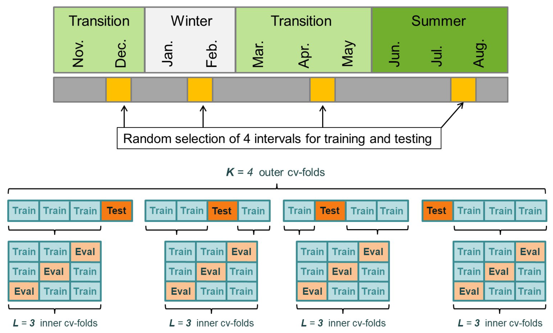
2.2.2. Sampling of Training Data and Cross-Validation

The data we had available spanned approximately ten months of continuous measurements, from the beginning of November to the end of August, with a one-hour temporal resolution. In most practical scenarios, obtaining such long continuous measurements from a single barn would be prohibitively expensive. Instead, three to six measurement periods, each lasting 1–14 days, would typically be carried out. A central aim of our study is to understand how different measurement scenarios (that is, choices of how often, how long, and at what times during the year measurement data is recorded) affect the resulting model. We simulated different measurement scenarios by randomly picking three, four, and six periods with lengths of one, seven, and fourteen days, respectively, under the constraint of including predetermined seasons. Here, the seasons were defined as summer (June to August, with night temperature around 11 °C and day temperature around 21 °C), winter (January and February, with night temperature around −2 °C and day temperature around 3 °C), and transition (March to May and September to December, with night temperature around 3 °C and day temperature around 10 °C). An overview of the 27 measurement scenarios is given in

Table 1. Overview of the 27 measurement scenarios studied in the empirical evaluation of the models. Index refers to the scenario index (1–27), plotted on the x-axis in most of the following figures. The columns of the table list the number of days for which measurements were recorded per period ($n_{\mathrm{days}}$), the number of measurement periods ($n_{\mathrm{periods}}$), and the distribution of measurement periods over the seasons: Transition ($n_{\mathrm{transition}}$), summer ($n_{\mathrm{summer}}$), and winter ($n_{\mathrm{winter}}$).

Index	${\mathit{n}}_{\mathbf{days}}$	${\mathit{n}}_{\mathbf{periods}}$	${\mathit{n}}_{\mathbf{transition}}$	${\mathit{n}}_{\mathbf{summer}}$	${\mathit{n}}_{\mathbf{winter}}$
1, 2, 3	1, 7, 14	3	1	1	1
4, 5, 6	1, 7, 14	4	2	1	1
7, 8, 9	1, 7, 14	4	2	2	0
10, 11, 12	1, 7, 14	4	3	1	0
13, 14, 15	1, 7, 14	6	2	2	2
16, 17, 18	1, 7, 14	6	3	2	1
19, 20, 21	1, 7, 14	6	4	1	1
22, 23, 24	1, 7, 14	6	4	2	0
25, 26, 27	1, 7, 14	6	5	1	0

.

In a practical scenario, the available data from the three to six measurement periods have to be used to train a statistical or machine learning model, optimize possible hyperparameters of the model, and obtain an estimate of its prediction error. We therefore studied a nested cross-validation protocol where an outer cross-validation loop serves to estimate the extrapolation error and an inner cross-validation loop is used to optimize model hyperparameters. The protocol is visualized in Figure 1. Of the three to six available measurement periods, one period was used as the outer cross-validation test set (denoted “Test” in Figure 1), one period was used as the inner cross-validation test set (denoted “Eval” in Figure 1), and the remaining periods were used as training sets in the inner cross-validation (denoted “Train” in Figure 1). The splitting into training, validation, and test sets was done using GroupShuffleSplit from scikit-learn [27]. For each training performed in the outer cross-validation loop, the hyperparameters of the models were optimized in the inner cross-validation by training models with different hyperparameters (see Section 2.2.1 for a description of the hyperparameters for each method) on the inner cross-validation training sets and evaluating them on the inner cross-validation test sets (“Eval”). The best hyperparameter configuration was then used to re-train a model on the outer training set, whose error was measured on the outer test set. As we had approximately 40 weeks of continuous measurement data available, in our scenario, we could also evaluate the model on all of the data not included in the training and test sets of the outer cross-validation (grey periods in the upper part of Figure 1). In the following, we refer to this error measurement as the extrapolation error. To this end, we optimized the hyperparameters of the model again on the outer cross-validation and re-trained the model on all of the selected data (orange periods in upper part of Figure 1).

2.2.3. Evaluation Measures

The measured performance of a modeling approach depends on the selected set of training data and on the evaluation criterion, where different measures highlight different properties. In order to study the influences of these two factors, we considered 30 realizations (i.e., random combinations) of each scenario defined in Table 1. We calculated means, standard deviations, quartiles, and interquartile ranges from those realizations. Moreover, we considered four different measures of model accuracy or goodness of fit, respectively.

The first three measures are based on evaluating predictive accuracy on individual test data points, that is, the hourly measurements of ammonia emissions in the test data. Very popular among those measures is the R² value (coefficient of determination). It provides the ratio of the average model error and the error of only averaging. It is based on calculating squared distances and thus weights individual outliers particularly strongly. Predictive performance can also be quantified in terms of different error measures that characterize the distance between the predicted and actual values for a test instance, where smaller values indicate a better model. Common error measures are the root mean squared error (RMSE) and the mean absolute error (MAE). RMSE provides the square root of the average squared difference between the predicted and the observed values, and incorporates the variance of the estimator and its bias. As in the case of R², strong outliers are weighted particularly strongly when using this measure. The MAE provides an average of the absolute differences between the predicted and the observed values. It weights all individual differences equally in the averaging. Hence, it is less sensitive to outliers than the RMSE and R².

The fourth measure, total absolute error (TAE), quantifies how closely the aggregated predicted emission values over the full ten-month period match the actual total emission value observed in the data. To optimize this measure, a model does not need to accurately predict the individual hourly emissions, but rather needs to correctly predict the total (or, equivalently, average) emissions over the full ten-month period. Formally, we define TAE as the absolute difference between the average model prediction over the ten-month period and the true average emissions observed in the data over this period. Achieving a low TAE is an important property of a model when the goal is to estimate aggregate yearly emissions. Because TAE is based on aggregating predictions over the entire ten-month period, it is less sensitive to outliers and fluctuations in the predictions. In the following, we will either present numerical TAE values or plot the average predicted emissions over the full ten-month period in comparison with the average true emissions over the ten-month period.

2.2.4. Graphical Representations

Confidence plots show the one-sigma interval of the predictions ($\mu \pm \sigma$, where $\mu$ is the mean value and $\sigma$ is the standard deviation). In box plots, the boxes extend from the lower to the upper quartile values of the data, with a horizontal orange line at the median. The whiskers extend from the box to show the range of the data. The upper whisker extends to the last datum less than $Q_3+w·\Delta Q$, where $Q_3$ is the upper quartile limit, $\Delta Q=Q_3-Q_1$ the interquartile range, and $w=1.5$. Analogously, the lower whisker extends to the first datum greater than $Q_1-w·\Delta Q$. Beyond the whiskers, data are considered as outliers and are plotted as individual points (circles). All visualizations were created using Matplotlib, version 3.0.3 [42].

3. Results

3.1. Prediction Accuracy

In Figure 2, the logarithm of the average predicted emissions over the ten-month period for the 27 basic scenarios (Table 1) is shown. Results are averaged over the 30 random realizations for each scenario; the light blue dashed lines show one-sigma intervals over these random realizations. The horizontal red lines show the logarithm of the average true emissions over the ten months observed in the data (${\overline{E}}_n$ = 1.406 g h⁻¹ LU⁻¹). In row 1, the results of the ensemble methods (gradient boosting and random forest) are shown; these two results are almost identical. In row 2, the results of linear regression with regularization (Ridge, left) and without regularization (LinReg, right) are shown. These results are very different from each other. For the linear regression case without regularization, many points are out of any reasonable range, particularly when only one day per measurement period is used. The results of the other scenarios, particularly those with six measurement periods, are more comparable to the results of the scenarios in row 1 and are considerably closer to the true ten-month averaged value. In principle, with regularization, the linear regression shows the same behavior as the ensemble methods when changing from one scenario to another, but all mean values are below the observed value. In row 3, the results for an artificial neural network with hyperparameter tuning (ANN, left) and a simple neural network with one hidden layer and four nodes (fixAnn, right) are shown. The predictions of the more complex ANN are generally much closer to the experimental value, and the variance is much lower than with the simplified version. The prediction of the fixAnn approach is, however, comparable to and in many cases better than that of the linear regression. In row 4, the predictions of the Gaussian process model (GaussProc, left) and the support vector machine (SVM, right) are shown. The variance of the Gaussian process is the lowest of all methods, but all mean values are below the experimental value. The predictions of the SVM are in most cases better than those of the simple neural network and the ordinary linear regression, but worse than those of the gradient boosting, random forest, Gaussian process, complex ANN, and ridge regression.

3.2. Evaluation Criterion and Model Selection

In addition to studying the accuracy with which average emissions can be predicted as presented in the previous subsection, we now study the predictive performance of the four best-performing regression methods with respect to different error measures. Figure 3 shows the train, test, and extrapolation mean absolute errors (MAE) for the four methods. Here, train error refers to the performance of the model during training, test error is the error estimate derived from the outer cross-validation, and extrapolation error refers to the error on the data disjoint from the train and test data (see Section 2.2.2). We observe that the extrapolation errors of gradient boosting and ridge regression are comparable, while that of the Gaussian process is smaller and fluctuates less. The complex ANN has the largest and most fluctuating extrapolation error. The test error slightly overestimates the extrapolation error in all cases. Although the Gaussian process has the lowest variance in the predicted emissions and the lowest test and extrapolation errors, the predicted average emission values are systematically too low (see Figure 2). Gradient boosting and random forest give the best predictions for the average emissions accompanied by the second-smallest mean absolute errors. The gradient-boosting algorithm is much faster than the random forest; hence, we focus on the gradient-boosting algorithm for further analysis.

Table 2. Mean absolute error (MAE), root mean square error (RMSE), coefficient of determination (R²), and total absolute error (TAE) measures for gradient boosting on the data disjoint from the training and test sets (TAE in g h⁻¹ LU⁻¹ and %, respectively; MAE and RMSE in ln [ g h⁻¹ LU⁻¹]; R² is dimensionless). The best and second-best results are marked in red and blue, respectively; the worst results are in boldface. Note: The 2 minimum errors of MAE, RMSE, and R² are obtained for index numbers 15 and 21, but for TAE, index numbers 22 and 24 give the smallest errors.

Scenario Unit	MAE ln [g h−1 LU−1]	RMSE 1	R2	TAE g h−1 LU−1	TAE %
1	0.441	0.350	0.236	0.0782	5.6
2	0.428	0.333	0.260	0.0830	5.9
3	0.409	0.314	0.297	0.0519	3.7
4	0.413	0.314	0.318	0.0747	5.3
5	0.404	0.303	0.335	0.0780	5.6
6	0.391	0.291	0.359	0.0437	3.1
7	0.480	0.418	0.088	0.0413	2.9
8	0.449	0.373	0.182	0.0716	5.1
9	0.473	0.400	0.127	0.0456	3.2
10	0.459	0.376	0.180	0.0277	2.0
11	0.428	0.343	0.256	0.0258	1.8
12	0.399	0.304	0.346	0.0232	1.7
13	0.427	0.324	0.292	0.1461	10.4
14	0.399	0.298	0.341	0.0899	6.4
15	0.376	0.271	0.398	0.0537	3.8
16	0.423	0.330	0.280	0.0651	4.6
17	0.394	0.296	0.346	0.0609	4.3
18	0.401	0.299	0.332	0.0626	4.5
19	0.416	0.316	0.312	0.0998	7.1
20	0.395	0.292	0.363	0.0759	5.4
21	0.378	0.270	0.402	0.0586	4.2
22	0.426	0.332	0.276	0.0047	0.3
23	0.418	0.323	0.302	0.0133	1.0
24	0.407	0.309	0.336	0.0125	0.9
25	0.425	0.334	0.272	0.0253	1.8
26	0.399	0.296	0.352	0.0582	4.1
27	0.392	0.287	0.388	0.0472	3.4

shows the MAE, RMSE, R², and TAE for the different scenario indices (compare with Table 1) for the gradient-boosting method on the data disjoint from the training and test sets. The best-performing scenario using the MAE measure is scenario 15 (i.e., six measurement periods with 14 days, equally distributed among the seasons). The second-best scenario is scenario 21 (i.e., six measurement periods with 14 days, out of which one period is in summer and one in winter). Using the RMSE or R², the two best-performing methods just change places. Considering the TAE, however, the ranking is completely different. Here, scenarios 22 and 24 are the best-performing scenarios (i.e., six measurement periods with 1 and 14 days, respectively, out of which two periods are in summer and four in the transition season).

3.3. Scenarios of Temporal Sampling

In Figure 4, the performance of the four best-performing methods over the different measurement scenarios and their realizations are compared in more detail using box plots. The figure shows the variability of the predicted average emission values for the different scenarios defined in Table 1 using gradient boosting, linear regression with regularization, an artificial neural network with hyperparameter tuning, and Gaussian processes, respectively. On average, the estimated ten-month emission value is close to the actually measured value (i.e., in all cases, the deviation from the experimental value is below 20%, often considerably less), even with the smallest datasets (i.e., in the scenario with three instances of one day).

The distribution of the estimated emission values around the mean is, however, broad in many cases. Taking six periods usually results in a lower variability of the estimation compared to taking three or four periods. Extending the considered measurement period (i.e., the number of training data per period) from one day to seven days decreases the variability in all sampling strategies. A further extension of the measurement duration to 14 days yields only little further improvement in most cases. The ranking of the scenarios differs among the regression methods, but the scenarios 2, 11, 12, 23, 24, 26, and 27 are typically among the best performing with regard to the mean estimated values. Among those, the scenario 12 shows the lowest variability.

Focusing only on the gradient-boosting method, which shows the best overall performance, in Figure 5, we show a detailed ranking of the scenarios with regard to the predicted ten-month emission value and the model extrapolation error (based on the MAE). In the upper part of the figure, we see that the scenarios 22, 24, 25, and 12 show very similar mean values which are close to the actually measured ten-month emission value. Among those four scenarios, the lowest variance is observed with scenario 24, followed by scenario 12. In the lower part of Figure 5, the ranking of the scenarios 15 and 21 is clearly the highest. Those scenarios are, however, closely followed by the scenarios 6, 27, 17, 20, 26, 12, 14, 18, and 5, which all show very similar mean extrapolation errors.

Except for the scenarios 25 and 22, which are highly ranked by TAE (but are low in terms of model error), there are no scenarios with only one day of measurements per period among the best-performing scenarios. In contrast, most of the scenarios with 14 days of measurements per period are highly ranked. There is no scenario with only three measurement periods among the best-performing scenarios in the detailed ranking. The only scenario that is ranked relatively highly by both TAE and model error is scenario 12 (that is, four measurement periods of 14 days each, out of which one is in summer and three are in the transition periods).

Finally, we consider the effect of the temporal distance between the measurement periods. As shown in Figure 6, the variability of the error decreases when increasing the minimal distance between the measurement periods. At the same time, in general, smaller errors are observed if there are at least 10 days between two measurement periods. A similar trend, although less pronounced, is observed when increasing the maximal distance between two measurement periods (color-coded in Figure 6).

4. Discussion

4.1. Importance of Temporal Sampling and Added Value of Machine Learning

Almost all modeling approaches tended to underestimate the aggregated emission value. Depending on the sampling scenario (selection of training periods) and realization, over- and underestimation occurred. The variability of the estimated emission values between the 30 random realizations of each scenario were large in many cases. This means that the probability of selecting a suboptimal training period — that is, a training period that leads to a large deviation between estimated and actual measurement values — was high, even for a scenario with six measurement periods of two weeks each.

On the other hand, our results indicate that an elongation of the measurement time from one week to two weeks yields, on average, only little improvement of the prediction performance, while the change from one day to one week usually reduced the variability around the mean of the emission estimations considerably. This is consistent with the results of Kafle et al., who showed that measurement protocols with one week every two months capture almost all of the variability of a dataset with measurements of one week every month [19]. In contrast, when considering only one day every two months, the authors did not capture the extremes, which may reduce the accuracy of any model that would be trained on the reduced dataset. Nevertheless, the emission values obtained with all sampling protocols in the case study of Kafle et al. were within ±20% of the relative bias of the baseline values, which is very similar to the range of errors observed in our case study.

In addition to the results described in the literature, our case study showed that the variability (error range) among the possible sampling strategies was higher with an ordinary linear regression (in most cases, even if regularization is added) compared to the other tested methods from the portfolio of machine learning. This is well in line with the conclusions of Wang et al., who found that the ammonia emission levels estimated with a standard statistical approach and with a simple artificial neural network were both consistent with measurements and literature values, but the prediction of the emissions (in terms of correlation with measurements) in their case study was slightly better with the neural network [21]. In addition, our study highlighted that with suitable hyperparameter tuning, the deviation in the performance of both methods can be further increased. Our results also showed that there are scenarios (that is, temporal sampling strategies) where both methods perform more similarly than in other scenarios. In particular, if a short measurement duration of only one day was used, the ordinary multilinear regression usually failed to reproduce the correct emission value. Since the prediction became considerably better when including a regularization, the failure of the ordinary multilinear regression was very likely induced by measurement noise. Thus, with linear regression and short measurement periods, reasonable results for the emission estimation can only be expected with a careful plausibility check and sound removal of outliers. The other tested methods were much more robust. In particular, the ensemble methods (for example, gradient boosting), which have not yet been used in the context of regression modeling of ammonia emissions, provided very robust estimates close to the actual emission value.

4.2. Sound Selection of Model Evaluation Criteria

The measured ten-month emission value, found to be 1.406 g h⁻¹ LU⁻¹ in this case study, was considered as a reference value here. Usually, such a reference value is not available for a measurement site. As an alternative, results from the aggregation based on short temporal samples are often compared to literature values. In our case, we found that the actually measured ten-month emission value, as well as the predicted mean emission value, were well in line with the range of annually averaged ammonia emission values found in literature, where values between 0.2 g h⁻¹ LU⁻¹ and 2.8 g h⁻¹ LU⁻¹ were reported [9,10,11,16,19]. The range in literature was, however, huge. This uncertainty has to be accepted not only due to the diverse measurement conditions, but also due to a large variation in barn design, management, and herd composition in the different studies.

On the other hand, the predicted mean emission value deviated from the actually measured ten-month emission value in most combinations of regression methods and sampling scenarios by less than 20%, which was regarded as an adequate error range for application purposes in contemporary literature [19]. Even when subtracting or adding 20%, our average emission would still be in the range reported in literature.

This error value of 20% is closely linked to the TAE, which focuses only on the aggregated emission value. With regard to an annual emission value the scenarios 12, 22, 24, and 25 showed the best performance, all of which were scenarios where no winter measurements, but many measurements in the transition time, were included (such as, for example, in the studies of Joo et al. in 2015 or Ngwabie et al. in 2014 [15,16]).

A totally different ranking of the sampling scenarios, however, resulted from the common measures of model accuracy or goodness of fit (i.e., MAE, RMSE, or R²), respectively. Among those measures, which evaluate to some degree how well the variability of the modeled time series is in line with that of the measured time series, the ranking was rather similar (see Table 2). In order to represent the dynamics of the emissions, the scenarios 15 and 21 were the most recommendable, i.e., those scenarios with rather equally distributed sampling over the seasons. Such a sampling would be in line, for example, with the recommendation in the VERA (i.e., Verification of Environmental Technologies for Agricultural Production) protocol for housing systems [13].

Independently of the error measure, almost all of the best-performing scenarios had six measurement periods, which supports the VERA recommendation of considering at least six periods. In contrast, the scenarios with six periods but only one day of measurements belong to the poorly performing scenarios. Number 13 (Table 1) is even one of the two worst-performing scenarios in Table 2. However, our study highlighted that how those periods should be distributed over the year considerably depends on the research question. For example, if we are interested in an emission factor of a husbandry system, a sampling that is associated with a low TAE is valuable. On the other hand, if we would like to predict the emissions of a building in certain weather conditions, for example, in order to implement a control strategy in terms of precision farming, the TAE is less important. In such a situation, a temporal sampling strategy that permits the training of a model that captures the emission dynamics (e.g., indicated by high $R^2$ values) would be more valuable. Thus, the model evaluation criterion must be selected accordingly. In contrast, the required length of the measurement periods is more closely related to the selected regression method and less dependent on the evaluation criterion.

5. Conclusions

We found that the deviation of the predicted mean emission values from the actually measured ten-month emission value was, in most combinations of regression methods and sampling scenarios, clearly below 20% (confirming our initial hypothesis 1). Only the ordinary multilinear regression in combination with scenarios of only one day of hourly measurements per period failed completely to project reasonable emission values. The model projection became more robust with longer measurement durations. Using multilinear regression with regularization made the model projections even more robust, but led to a systematic underestimation of the mean emission value. It has to be noted that a similar behavior can be expected if ordinary multilinear regression is applied to a dataset where all outliers have been removed beforehand (as such a procedure could be understood as a manual regularization). The performance of artificial neural networks and support vector regression was ranked in the intermediate places. The Gauss process had the lowest variance in the predicted emission mean values and the lowest test and extrapolation errors, but the predicted mean values were systematically too low. The ensemble methods of gradient boosting and random forests gave the best predictions for the emissions, accompanied by the second-smallest errors. This confirmed our initial hypothesis 2, that machine learning approaches can improve emission predictions. Concerning the temporal sampling, our study showed that at least seven days of hourly measurements per period are advisable for robust predictions. Scenarios with four or six measurement periods clearly outperformed scenarios with only three measurement periods. Common measures of model accuracy (MAE, RMSE, or R²) were not meaningful with regard to the quality of the predicted aggregated emission values (as measured by TAE). Consequently, although most of the highly ranked scenarios involved six measurement periods, taking into account scenarios that were highly but not top-ranked by all four measures, we concluded that the scenario with the best overall performance was: Four measurement periods, each lasting for 14 days, where one period was in summer and three were in the transition periods. A minimal temporal distance of at least 10 days between two consecutive periods was valuable.

Further in-depth studies on the effects of temporal sampling are advisable in order to better understand the observed trends in the model accuracy when changing the number and duration of measurement periods.

References

1. Sutton, M.A.; Bleeker, A.; Howard, C.; Erisman, J.; Abrol, Y.; Bekunda, M.; Datta, A.; Davidson, E.; de Vries, W.; Oenema, O.; et al. Our Nutrient World. The Challenge to Produce More Food & Energy with Less Pollution; Technical Report; Centre for Ecology & Hydrology: Edinburgh, UK, 2013. [Google Scholar]
2. Hempel, S.; Menz, C.; Pinto, S.; Galán, E.; Janke, D.; Estellés, F.; Müschner-Siemens, T.; Wang, X.; Heinicke, J.; Zhang, G.; et al. Heat stress risk in European dairy cattle husbandry under different climate change scenarios—Uncertainties and potential impacts. Earth Syst. Dyn. 2019, 10, 859–884. [Google Scholar] [CrossRef] [Green Version]
3. Amon, B.; Kryvoruchko, V.; Amon, T.; Zechmeister-Boltenstern, S. Methane, nitrous oxide and ammonia emissions during storage and after application of dairy cattle slurry and influence of slurry treatment. Agric. Ecosyst. Environ. 2006, 112, 153–162. [Google Scholar] [CrossRef]
4. Monteny, G.; Groenestein, C.; Hilhorst, M. Interactions and coupling between emissions of methane and nitrous oxide from animal husbandry. Nutr. Cycl. Agroecosyst. 2001, 60, 123–132. [Google Scholar] [CrossRef]
5. Hristov, A.N. Contribution of ammonia emitted from livestock to atmospheric fine particulate matter (PM2.5) in the United States. J. Dairy Sci. 2011, 94, 3130–3136. [Google Scholar] [CrossRef]
6. European Environment Agency (EEA). European Union Emission Inventory Report 1990–2017; European Environment Agency: Copenhagen, Denmark, 2019; Volume 8. [Google Scholar]
7. Sanchis, E.; Calvet, S.; del Prado, A.; Estellés, F. A meta-analysis of environmental factor effects on ammonia emissions from dairy cattle houses. Biosyst. Eng. 2019, 178, 176–183. [Google Scholar] [CrossRef]
8. Calvet, S.; Gates, R.S.; Zhang, G.Q.; Estellés, F.; Ogink, N.W.; Pedersen, S.; Berckmans, D. Measuring gas emissions from livestock buildings: A review on uncertainty analysis and error sources. Biosyst. Eng. 2013, 116, 221–231. [Google Scholar] [CrossRef] [Green Version]
9. Schrade, S.; Zeyer, K.; Gygax, L.; Emmenegger, L.; Hartung, E.; Keck, M. Ammonia emissions and emission factors of naturally ventilated dairy housing with solid floors and an outdoor exercise area in Switzerland. Atmos. Environ. 2012, 47, 183–194. [Google Scholar] [CrossRef]
10. Wu, W.; Zhang, G.; Kai, P. Ammonia and methane emissions from two naturally ventilated dairy cattle buildings and the influence of climatic factors on ammonia emissions. Atmos. Environ. 2012, 61, 232–243. [Google Scholar] [CrossRef]
11. Hempel, S.; Saha, C.K.; Fiedler, M.; Berg, W.; Hansen, C.; Amon, B.; Amon, T. Non-linear temperature dependency of ammonia and methane emissions from a naturally ventilated dairy barn. Biosyst. Eng. 2016, 145, 10–21. [Google Scholar] [CrossRef] [Green Version]
12. Dekock, J.; Vranken, E.; Gallmann, E.; Hartung, E.; Berckmans, D. Optimisation and validation of the intermittent measurement method to determine ammonia emissions from livestock buildings. Biosyst. Eng. 2009, 104, 396–403. [Google Scholar] [CrossRef]
13. International VERA Secretariat. VERA TEST PROTOCOL for Livestock Housing and Management Systems, 3rd ed.; International VERA Secretariat: Delft, The Netherlands, September 2018. [Google Scholar]
14. Eurich Menden, B.; Wolf, U.; Gallmann, E. Ermittlung von Emissionsdaten für die Beurteilung der Umweltwirkungen der Nutztierhaltung - EmiDaT. Poster at the BTU Conference. 2017. Available online: https://www.ktbl.de/fileadmin/user_upload/Allgemeines/Download/EmiDaT/Poster-EmiDaT.pdf (accessed on 4 December 2019).
15. Joo, H.; Ndegwa, P.; Heber, A.; Ni, J.Q.; Bogan, B.; Ramirez-Dorronsoro, J.; Cortus, E. Greenhouse gas emissions from naturally ventilated freestall dairy barns. Atmos. Environ. 2015, 102, 384–392. [Google Scholar] [CrossRef]
16. Ngwabie, N.M.; Vanderzaag, A.; Jayasundara, S.; Wagner-Riddle, C. Measurements of emission factors from a naturally ventilated commercial barn for dairy cows in a cold climate. Biosyst. Eng. 2014, 127, 103–114. [Google Scholar] [CrossRef]
17. König, M.; Hempel, S.; Janke, D.; Amon, B.; Amon, T. Variabilities in determining air exchange rates in naturally ventilated dairy buildings using the CO2 production model. Biosyst. Eng. 2018, 174, 249–259. [Google Scholar] [CrossRef]
18. Ulens, T.; Daelman, M.R.; Mosquera, J.; Millet, S.; van Loosdrecht, M.C.; Volcke, E.I.; Van Langenhove, H.; Demeyer, P. Evaluation of sampling strategies for estimating ammonia emission factors for pig fattening facilities. Biosyst. Eng. 2015, 140, 79–90. [Google Scholar] [CrossRef]
19. Kafle, G.K.; Joo, H.; Ndegwa, P.M. Sampling Duration and Frequency for Determining Emission Rates from Naturally Ventilated Dairy Barns. Trans. ASABE 2018, 61, 681–691. [Google Scholar] [CrossRef]
20. Saha, C.; Ammon, C.; Berg, W.; Fiedler, M.; Loebsin, C.; Sanftleben, P.; Brunsch, R.; Amon, T. Seasonal and diel variations of ammonia and methane emissions from a naturally ventilated dairy building and the associated factors influencing emissions. Sci. Total Environ. 2014, 468, 53–62. [Google Scholar] [CrossRef]
21. Wang, C.; Li, B.; Shi, Z.; Zhang, G.; Rom, H. Comparison between the Statistical Method and Artificial Neural Networks in Estimating Ammonia Emissions from Naturally Ventilated Dairy Cattle Buildings. In Proceedings of the Livestock Environment VIII, Iguassu Falls, Brazil, 31 August–4 September 2008; American Society of Agricultural and Biological Engineers: St. Joseph, MI, USA, 2009; p. 7. [Google Scholar]
22. Boniecki, P.; Dach, J.; Pilarski, K.; Piekarska-Boniecka, H. Artificial neural networks for modeling ammonia emissions released from sewage sludge composting. Atmos. Environ. 2012, 57, 49–54. [Google Scholar] [CrossRef]
23. Stamenković, L.J.; Antanasijević, D.Z.; Ristić, M.Đ.; Perić-Grujić, A.A.; Pocajt, V.V. Modeling of ammonia emission in the USA and EU countries using an artificial neural network approach. Environ. Sci. Pollut. Res. 2015, 22, 18849–18858. [Google Scholar] [CrossRef]
24. Liakos, K.; Busato, P.; Moshou, D.; Pearson, S.; Bochtis, D.D. Machine Learning in Agriculture: A Review. Sensors 2018, 18, 2674. [Google Scholar] [CrossRef] [Green Version]
25. Janke, D.; Willink, D.; Hempel, S.; Ammon, C.; Amon, B.; Amon, T. Influence of Wind Direction and Sampling Strategy on the Estimation of Ammonia Emissions in Naturally Ventilated Barns. In New Engineering Concepts for Valued Agriculture; Groot Koerkamp, P., Lokhorst, C., Ipema, A., Kempenaar, C., Groenestein, C., van Oostrum, C., Ros, N., Eds.; Wageningen University and Research: Wageningen, The Netherlands, 2018; pp. 762–767. [Google Scholar]
26. Pedersen, S.; Sällvik, K. Climatization of Animal Houses. Heat and Moisture Production at Animal and House Levels; Research Centre Bygholm, Danish Insitute of Agricultural Sciences: Horsens, Denmark, 2002; pp. 1–46. [Google Scholar]
27. Pedregosa, F.; Varoquaux, G.; Gramfort, A.; Michel, V.; Thirion, B.; Grisel, O.; Blondel, M.; Prettenhofer, P.; Weiss, R.; Dubourg, V.; et al. Scikit-learn: Machine Learning in Python. J. Mach. Learn. Res. 2011, 12, 2825–2830. [Google Scholar]
28. Quinlan, J.R. Induction of decision trees. Mach. Learn. 1986, 1, 81–106. [Google Scholar] [CrossRef] [Green Version]
29. Ho, T.K. Random Decision Forests. In Proceedings of the 3rd International Conference on Document Analysis and Recognition, Montreal, QC, Canada, 14–16 August 1995; pp. 278–282. [Google Scholar]
30. Breiman, L. Arcing The Edge; Technical Report 486; Statistics Department, University of California: Berkeley, CA, USA, 1997. [Google Scholar]
31. Friedman, J.H. Greedy Function Approximation: A Gradient Boosting Machine; Ims 1999 Reitz Lecture; Sequoia Hall, Stanford University: Stanford, CA, USA, 1999; Available online: http://statweb.stanford.edu/~jhf/ftp/trebst.pdf (accessed on 4 December 2019).
32. Hoerl, A.E. Application of ridge analysis to regression problems. Chem. Eng. Prog. 1962, 58, 54–59. [Google Scholar]
33. McCulloch, W.S.; Pitts, W. A logical calculus of the ideas immanent in nervous activity. Bull. Math. Biophys. 1943, 5, 115–133. [Google Scholar] [CrossRef]
34. Rosenblatt, F. The Perceptron: A Probabilistic Model For Information Storage And Organization In The Brain. Psychol. Rev. 1958, 65, 386–408. [Google Scholar] [CrossRef] [Green Version]
35. Werbos, P. Beyond Regression: New Tools for Prediction and Analysis in the Behavioral Sciences; Harvard University: Cambridge, MA, USA, 1975. [Google Scholar]
36. Rumelhart, D.E.; Hinton, G.E.; Williams, R.J. Learning representation by back-propagating errors. Nature 1986, 323, 533–536. [Google Scholar] [CrossRef]
37. Glorot, X.; Bordes, A.; Bengio, Y. Deep Sparse Rectifier Neural Networks. In Proceedings of the Fourteenth International Conference on Artificial Intelligence and Statistics, Fort Lauderdale, FL, USA, 11–13 April 2011; Gordon, G., Dunson, D., Dudík, M., Eds.; Proceedings of Machine Learning Research: London, UK, 2011; Volume 15, pp. 315–323. [Google Scholar]
38. Kingma, D.P.; Ba, J. Adam: A Method for Stochastic Optimization. arXiv 2014, arXiv:1412.6980. Available online: https://arxiv.org/abs/1412.6980 (accessed on 20 January 2020).
39. Cortes, C.; Vapnik, V. Support-Vector Networks. Mach. Learn. 1995, 20, 273–297. [Google Scholar] [CrossRef]
40. Drucker, H.; Burges, C.J.C.; Kaufman, L.; Smola, A.J.; Vapnik, V. Support Vector Regression Machines. In Advances in Neural Information Processing Systems 9; NIPS: Denver, CO, USA, 1996; pp. 155–161. [Google Scholar]
41. Rasmussen, C.E.; Williams, C.K.I. Gaussian Processes for Machine Learning (Adaptive Computation and Machine Learning); The MIT Press: Cambridge, MA, USA, 2005. [Google Scholar]
42. Hunter, J.D. Matplotlib: A 2D graphics environment. Comput. Sci. Eng. 2007, 9, 90–95. [Google Scholar] [CrossRef]
Figure 1. Sketch of the nested cross-validation protocol used for hyperparameter tuning and error estimation for the scenario of four measurement periods, randomly selected from the whole measurement period (November 2016–September 2017). With these four selected periods, an outer K-fold cross-validation ( K = 4 ) for the estimation of the generalization error and an inner L-fold cross-validation ( L = 3 ) for the hyperparameter tuning are performed.
Sustainability 12 01030 g001
Figure 2. Logarithm (natural) of the average predicted emissions over the full ten-month period in ln [g h−1 LU−1] for different measurement scenarios and eight different regression methods. The red horizontal lines show the logarithm of the true average emission value observed in the experimental dataset. The blue points (and lines) are averaged over the 30 random realizations of each scenario. The light blue dashed lines show the one-sigma intervals over the 30 random realizations. Please note the different scalings of the y-axes.
Sustainability 12 01030 g002
Figure 3. Comparison of mean absolute error (all in ln [g h−1 LU−1]) for the four best-performing regression methods. The mean values of training (orange) and test error (red) from the cross-validation are compared. In addition, the extrapolation error (blue) of the retrained model for the data disjoint from the training and test sets is shown for comparison. All error values depict averages over 30 random selections of training data in agreement with the scenario constraints.
Sustainability 12 01030 g003
Figure 4. Predicted average emissions (in g h−1 LU−1) for the four best-performing regression models. The average values and the variability based on the 30 random realizations are shown as box plots for the different scenarios. The red lines show the average emission value (1.406 g h−1 LU−1) that was observed in the complete experimental dataset. The lengths of the measurement periods of the individual scenarios are color-coded.
Sustainability 12 01030 g004
Figure 5. Scenario ranking based on the average predicted emissions and the mean absolute error of gradient boosting. In the upper figure, scenario indices are ordered according to descending average predicted emission value. In the lower figure, scenario indices are ordered according to ascending mean absolute extrapolation error (MAE). The ordering of the scenario indices is based on the average over the 30 realizations per scenario (brown bars); the width of the one-sigma interval is shown in orange and green. The red line in the upper panel corresponds to the ten-month average emission value observed in the data.
Sustainability 12 01030 g005
Figure 6. Model accuracy of gradient boosting as a function of the minimal ( d min ) and maximal ( d max ) distances in days between any two measurement periods for the different measurement scenarios and their realizations. In both panels, the x-axis corresponds to d min , and d max is color-coded. Left panel: Predicted average emissions depending on d min and d max . The red line corresponds to the ten-month emission value. Right panel: Mean absolute extrapolation error depending on d min and d max .
Sustainability 12 01030 g006