Abstract
To avoid conflicts among trains at stations and provide passengers with a periodic train timetable to improve service level, this paper mainly focuses on the problem of multi-periodic train timetabling and routing by optimizing the routes of trains at stations and their entering time and leaving time on each chosen arrival–departure track at each visited station. Based on the constructed directed graph, including unidirectional and bidirectional tracks at stations and in sections, a mixed integer linear programming model with the goal of minimizing the total travel time of trains is formulated. Then, a strategy is introduced to reduce the number of constraints for improving the solved efficiency of the model. Finally, the performance, stability and practicability of the proposed method, as well as the impact of some main factors on the model are analyzed by numerous instances on both a constructed railway network and Guang-Zhu inter-city railway; they are solved using the commercial solver WebSphere ILOG CPLEX (International Business Machines Corporation, New York, NY, USA). Experimental results show that integrating multi-periodic train timetabling and routing can be conducive to improving the quality of a train timetable. Hence, good economic and social benefits for high-speed rail can be achieved, thus, further contributing to the sustained development of both high-speed railway systems and society.
1. Introduction
High-speed railways that meet the requirements of the modern passenger market and sustainable development, compared with conventional railways, are a new type of green transportation due to their operating characteristics of high speed, high density, large capacity, low energy consumption and little pollution. Therefore, a more accurate and feasible train timetable is urgently needed to conduct train operation and provide passengers with high quality service. The train route allocation plan at stations is an important extension of train timetables and has an intimate interaction relationship with train timetables. As trains on a high-speed rail network create dense arrivals and departures at stations, train routing at stations on a high-speed rail network has much more influence on train timetabling compared with conventional railway. Moreover, in recent years, a multi-periodic train timetable has attracted more passengers as its regularity is greatly convenient for their travel. Thus, simultaneously studying multi-periodic timetabling and routing on high-speed railway networks has a great significance. First, the simultaneous optimization of the two problems can avoid operational conflicts occurring among different trains at stations, so as to improve the efficiency of trains’ operating and make the resource utilization of stations maximized at the same time. Moreover, eliminating conflicts can reduce the human resource workload to deal with the conflicts to improve the efficiency of management of the transportation system and decrease the cost of transportation organization and management on the high-speed railway network. Second, this can improve the quality of train timetables and help to serve passengers better, letting more passengers choose high-speed rail instead of conventional railways, cars, or airplanes. It is good for achieving the social and economic benefits of high-speed rail systems. Third, with the improvement of resource allocation at stations and elimination of conflicts among trains, the high-speed rail’s market competitiveness will be significantly improved. This is conducive to the healthy and sustained development of high-speed railways. In conclusion, integrating multi-periodic train timetabling and routing at stations can realize the reasonable utilization of resources at stations and improve the quality of train timetables to achieve good social and economic benefits of high-speed rail, which will contribute to the sustained development of both high-speed railway systems and society.
Generally, the problem of train timetabling is to determine the arrival and departure time of trains at their predetermined service stations, whereas the problem of train routing is concerned with the assignment of a travel path including an arrival–departure track to trains at each of their visited stations. Specifically, for train routing, operation paths for trains at their visited stations are arranged based on their arrival time and departure time obtained by timetabling, whereas train timetables usually need to be constantly adjusted in train routing to ensure that no conflicts will occur among different trains at stations, so as to realize reasonable utilization of station resources.
In existing research, most researchers aimed to optimize train timetabling at the cost of neglecting the layouts of stations and by viewing each station as a node. Alternatively, they scheduled trains based on pre-determined routes of trains at stations. Other researchers studied on solving the problem of train routing with a given train timetable; however, very few focused on the simultaneous optimization of train timetabling and routing, for it is usually too complicated to solve this problem, especially in face of large-scale examples. However, a train timetable that does not consider the routes of trains at a station is usually infeasible, as there may be conflicts among trains at these stations, which further leads to delays and other problems. Considering these issues, Mu and Dessouky [1] proposed a switchable strategy for trains to reduce delays among trains by using the reverse direction tracks. This is the optimization problem of train routing and timetabling collaboratively, which is called non-deterministic polynomial hard (see Cai and Goh [2], Caprara et al. [3], and Caimi et al. [4], who addressed the issue of generating conflict-free train schedules with consideration of conflicts when two or more than two trains were simultaneously arranged to the same track). Pellegrini et al. [5] focused on avoiding perturbation and sought the best train routing and scheduling. Xu et al. [6] carried out relevant research for the purpose of reducing train delay and improving the utilization rate of railway tracks.
In recent years, a periodic train timetable with a single operation period, whose trains’ arrival time and departure time need to satisfy the requirement of an identical headway, has been popular and widely used among developed countries for its easy-to-understand regularity, which is convenient for passengers to travel and organizers to arrange station operation work. For example, Sparing and Goverde [7] described a method for generating periodic timetables that can ensure maximum stability for a heterogeneous rail network. Nevertheless, in these kinds of train timetables, the flexibility of trains’ arrival and departure time drops because of the fixed interval and the same visited stations, with train stops among various operation periods. Hence, trains’ time–space distribution does not completely meet the time–space distribution of passenger demand. Moreover, there is sometimes a need to stop some trains, so that the decreasing passenger demand in non-peak periods is met, which decreases the regularity among trains.
A multi-periodic train timetable is another form of a periodic train timetable, and trains using this timetable must operate periodically with multiple headways. That is, trains having the same speed and stop plans are classed as a period-type and operate with an identical time interval; moreover, various period-types can have multiple operation time intervals. For instance, Odijk [8] said that trains with various destinations can travel according to various time-periods. Compared with a single periodic train timetable, trains using a multi-periodic train timetable not only have strict operation regularity, but also can better adapt to the change of passenger demand among various time periods by coordinating the departure time of each period-type’s first train at its origin station and the operating time horizon for each period-type’ trains.
However, very few existing studies of multi-periodic train timetabling have taken train routing at stations into account. Most researchers simplified each station as a node so that trains of the same period-type enter and leave a station node with an equivalent interval (e.g., Zhou and Yang [9] and Zhou and Tian [10]. As detailed above, train timetabling that considers train routing is necessary to efficiently avoid operational conflicts among different trains at stations. Obviously, it is also necessary to simultaneously optimize the multi-periodic train timetabling and routing.
Compared with the integrated aperiodic train timetabling and routing, the simultaneous multi-periodic train timetabling and routing has two significant differences.
- (1)
- It needs to search a specific travel path for each train at its each visited station and to make trains of the same period-type enter and leave off the same station with the same headway to let them operate periodically.
- (2)
- Trains of the same period-type travel with an identical headway, which is more than any minimum safety headways. Moreover, the sequence of these trains occupying tracks in either sections or at stations is constant. Therefore, the requirements of all types of safety time-intervals among them are automatically satisfied, so we only need to consider some safety intervals among trains of different period-types.
Our paper focuses on the multi-periodic train timetabling and routing simultaneously based on some predetermined trains of each period-type on a high-speed railway network including one-way and two-way tracks. It aims to optimizing not only the routes of all trains at their visited stations but also their entering and leaving time on visited sections and stations. The main difficulty is that we need to make trains of the same period-type enter and leave the same section or station with the same headway while searching routes for them at each visited station. This paper provides two main contributions for the optimization problem of train timetabling and routing.
- (1)
- A mixed integer linear programming model is formulated for the simultaneous multi-periodic train timetabling and routing, and the commercial solver WebSphere ILOG CPLEX (International Business Machines Corporation, New York, NY, USA) is applied to solve it. This model optimizes the entering time and leaving time of all trains and also searches for their routes of arrival–departure tracks at their visited stations.
- (2)
- A strategy is designed to partly predetermine the sequence of trains occupying the same arrival–departure track, and it is greatly useful to improve the solve efficiency of our model.
In this paper, Section 2 presents literature reviews about aperiodic and periodic train timetabling and routing. Section 3 shows the specific description for the problem of simultaneous multi-periodic train timetabling and routing. In Section 4, a mixed integer linear programming model is formulated for simultaneous multi-periodic train timetabling and routing, and the commercial solver WebSphere ILOG CPLEX (International Business Machines Corporation, New York, NY, USA) is applied to solve it. In Section 5, a simplified strategy is introduced to improve the solve efficiency of our model. In Section 6, some numerical examples based on both a constructed railway network and a case study of the Guangzhou–Zhuhai inter-city railway network are presented to illustrate the performance, efficiency, and stability of our proposed model. Finally, Section 7 gives the conclusions and further studies.
2. Literature Reviews
2.1. Reviews on Aperiodic Train Timetabling and Routing
As the integrated optimization of train timetabling and routing at stations is a non-deterministic polynomial-hard problem (Samà et al. [11]), most researchers preferred to optimize them respectively or interactively, and very few focused on their simultaneous optimization.
In the process of aperiodic train timetabling, some studies usually neglected the layouts of stations and viewed each station as a node with either considering transportation capacity or not, while others might schedule trains with pre-determined routes at stations. As to the first case, Mees [12] considered stations or track intersections as nodes to represent a railway network in train timetabling. Caprara et al. [3] proposed a directed multigraph, in which a station was represented by its departure and arrival nodes, to solve the problem of train timetabling. Törnquist and Persson [13] used a junction node between two adjacent sections to represent a station for single-track train re-scheduling. Regarding train timetabling with given train routes, Szpigel [14] built a mixed integer programming model with given departure times and routes of trains and solved the problem of train timetabling by designing a branch-and-bound algorithm. D’Ariano et al. [15] aimed to resolve the conflicts among trains using a timetable with fixed routes. Dessouky et al. [16] proposed a branch-and-bound method to optimize scheduling time for trains traveling with given routes on a complex rail network.
The problem of train routing generally is to optimize trains’ routes at their visited stations with a given train timetable. For instance, De Luca et al. [17] developed a heuristic technique, which is based on a graph-coloring algorithm, to choose routes and platforms for all or as many trains as possible, whose arrival and departure time were fixed. Zwaneveld et al. [18] decomposed the solving process of train routing problem into three steps—preprocessing, valid inequalities, and a branch-and-cut approach. What worthy noting is that it used a current timetable as an input. Based on a given timetable, Caimi, Burkolter, and Herrmann [19] addressed the routing of train passing through railway stations and outlined two algorithms. The first algorithm searched for a feasible solution in the problem of train routing and was modified in the second algorithm to increase the time slots of a chosen route. Lusby et al. [20] reviewed models and methods in finding routes for each train in each station with fixed arrival and departure time in a timetable. Taking into account the daily train timetables and the operational and structural constraints, Billionnet [21] assigned available tracks at stations to trains and designed an integer programming method.
However, a train timetable that does not consider the routing choices is usually infeasible, as there may be conflicts among trains at stations. As concluded by Goverde and Hansen [22] and Burggraeve and Vansteenwegen [23], with the lack of train scheduling, the problem of train routing is limited by already scheduled arrival times and departure times. Thus, some researchers aimed to optimize train timetabling and routing interactively and iteratively. For example, Mazzarello and Ottaviani [24] proposed a heuristic algorithm consisting of three steps. The first step was to solve a scheduling problem that only train sequence was allowed to be modified, the second step was to modify the routes, and the third step was to readjust the train timetable with the new chosen routes. Dewilde et al. [25] focused on the interaction between the train running routes through the station area and the timetable at stations within this area to minimize the real travel time and improve the robustness at railway stations. Lee, Yusin, and Chen [26] presented a heuristic algorithm to optimize train routing and train timetabling iteratively. It generated an initial solution with a simple rule, and then used a four-step process to adjust the solution iteratively. Castillo et al. [27] determined train timetables and train routes sequentially in order to reduce the complexities and difficulties of solving the problem on a double and single-tracked bidirectional railway network.
To some extent, such an interactive planning process may lead to poor coordination between train schedules and train routes and lead to departure delays. Therefore, simultaneous train timetabling and routing is better to construct an operational timetable. For this purpose, Morlok and Peterson [28] initially integrated the problem of the routing and scheduling into an optimization model. Li et al. [29] developed a single-objective train routing model combined with train scheduling and the model was solved by a Tabu search algorithm. Pellegrini et al. [5] designed a mixed integer linear programming model for finding the best train routing and dispatching in the event of disturbances in real-time rail traffic management. With the goal of improving the utilization rate of railway tracks and reducing train delay, Xu et al. [6] designed a simulation method based on discrete event model to generate high-quality train route and timetable strategies for trains. Zhou and Teng [30] focused on using an efficient train-based Lagrangian relaxation decomposition to optimize the problem of simultaneous train routing and timetabling.
2.2. Reviews on Periodic Train Timetabling and Routing
A periodic train timetable is widely used in developed countries due to its easy-to-understand regularity. Some studies such as Wardman et al. [31], Johnson et al. [32] also confirmed that the regularity of a timetable indeed helped attract passengers. Since Serafini and Ukovich [33] first dealt with the problem of fixed-traffic control with a model based on the theory of periodic event scheduling problem (PESP), most approaches to the problem of periodic train timetabling have been proposed on basis of PESP. For instance, Odijk [8] proposed a PESP-based algorithm for generating periodic train timetables. Goverde [34] reformulated PESP by taking buffer time as decision variables and utilized a graph structure to reduce the number of variables. Kroon and Peeters [35] assumed that the trip time of all trains on rail tracks were known beforehand, and then a PESP-based periodic train timetabling model was extended. Lindner [36] extended the PESP model by adding operating costs into the objective. Heydar, Petering, and Bergmann [37] developed a mixed integer linear programming model to minimize the length of the dispatching cycle and minimize the total stopping time of local trains at all stations. In addition to the PESP-based approaches, some researchers employed other methods to optimize a periodic train timetable. Nachtigall and Voget [38] proposed a genetic algorithm, which is a combination of greedy heuristic algorithm and a local improvement program, to minimize the waiting time in transfer. Caprara et al. [3] developed a method for optimizing a periodic train timetable on a single-track rail, which is represented by a directed graph. Sels, Cattrysse, and Vansteenwegen [39] optimized a periodic train timetable by employing a spanning tree method.
Moreover, similar to the problem of aperiodic train timetabling and routing, most of the existing literature is devoted to optimizing them respectively or interactively; however, very few studies have focused on their simultaneous optimization. Caimi et al. [4] considered the problem of timetabling at the macroscopic level and the problem of routing at stations at the microscopic level sequentially on a large rail network, then designed a two-level-elasticity PESP approach to solve this problem. Sparing and Goverde [7] assumed that the line pattern and routes of trains were fixed and generated feasible periodic train timetables with maximizing the stability of networks. Burggraeve and Vansteenwegen [23] first proposed an integer linear routing model to assign routes for each train and then designed a mixed integer linear timetabling model to assign a time for each train.
A common characteristic is that these studies all considered a periodic timetable with a cycle-time, such as one hour. However, very few studies are devoted to the optimization of multi-periodic train timetabling—that is, optimizing a periodic train timetable with multiple operation periods to better meet the operational constraints of different railway lines and the change in different time-periods of passenger demand. Odijk [8] and Nachtigall [40] first proposed trains with different destinations could have different operation cycles on a same railway network. Zhou and Yang [9], Zhou and Tian [10], and Zhou and Teng [30] aimed to solve the problem of multi-periodic train timetabling to optimize the operation periods and arrival and departure time of trains of all period-types on a double-track rail network. However, there have been no studies devoted to integrating multi-periodic train timetabling and routing.
To better understand the difference between the current exiting research and this paper, a summary table is given to display the main research on aperiodic train timetabling or routing, and periodic train timetabling or routing, as shown in Table 1.

Table 1.
Some main research on train timetabling and routing.
3. Problem Description
3.1. Representation of Rail Networks
3.1.1. Representation of a Physical Railway Network
A physical railway network consists of a set of stations and a set of sections, and it can usually be represented by nodes and a set of arcs. Each node represents an intersection point of section lines, station tracks, turnout lines, etc. Each arc connects two nodes, and it can be either unidirectional or bidirectional depending on whether its corresponding line or track can be traversed by trains from one direction or two opposite directions. Moreover, arcs can be classified as section arcs and station arcs according to sections and stations, and station arcs can be further classified as arrival–departure track arcs and non-arrival–departure track arcs. Note that arrival–departure track arcs can be used for trains to stay, overtake, and yield to other trains, and for passengers to get off and on trains, while section arcs and non-arrival–departure track arcs cannot.
Take the physical rail network shown in Figure 1 as an example. It consists of four stations, one unidirectional section, and two bidirectional sections. For the unidirectional section connecting station A and B, it contains two lines that are used by trains from up and down directions, respectively. However, the two-way section between station B and station C or between station B and station D has only one line, which can be used by trains from both up and down directions.
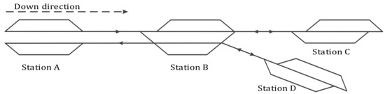
Figure 1.
A railway network consisting of four stations and three sections.
3.1.2. Representation of a Constructed Railway Network
Based on the physical rail network in Figure 1, Figure 2 gives the representation of a constructed rail network, which is represented by a directed graph including a group of nodes and various types of weighted directed arcs between nodes. From the Figure 2, it is obvious that the constructed rail network consists of both sections having one two-way track and sections having two one-way tracks.
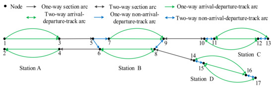
Figure 2.
A directed graph corresponding to Figure 1.
As illustrated in Figure 2, a set of nodes {1, 2, 3, 4}, {5, 6, 7, 8, 9}, {10, 11, 12, 13}, and {14, 15, 16, 17} are generated for stations A, B, C and D, respectively. Among them, nodes 3, 4 represent the intersection points of section lines and station tracks, and nodes 8, 9 show the junctions of switch lines, station tracks and section lines. A one-way arc, for example, arc (3, 5) only allows trains to run on it from a specific direction, whereas a two-way arc, such as arc (9, 10) or (8, 14), can service trains coming from two opposite directions. Moreover, section arcs (3, 5), (9, 10), and (8, 14) are created to show the movement of trains in sections A–B, B–C, and B–D, respectively, while arcs (1, 3) and (4, 2) are arrival–departure track arcs, and arcs (5, 6) and (5, 7) are non-arrival–departure track arcs.
3.2. Description of Multiple Period-Types of Trains
Trains that have the same origins, terminals, stops, and travel with the same period-length are viewed as trains of the same period-type. Moreover, trains of different period-types can have the same period-length or different period-lengths, and each period-type can have diverse number of trains. As demonstrated in Figure 3, there are two period-types with different period-lengths. Three trains of period-type 1 represented by dark blue lines will run with a given period-length, that is, 20 min, while four trains of period-type 2 denoted by red lines will run with the given period-length, that is, 10 min.
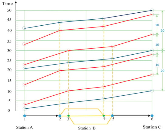
Figure 3.
A description graph consisting of double-periodic trains.
Specifically, as for trains of the same period-type, using the same headway, they not only depart from the same origin with the same period-length, but also arrive at and leave off the same visited station with the same period-length, and their dwelling time at their stopped stations are the same with each other as well. We take four trains in red for an example, the period-length between two adjacent trains is 10 min; thus, they respectively depart from station A at moment 3, 13, 23, and 33 and arrive at station B at moment 10, 20, 30, and 40. After a two-minute dwelling, then leave station B at moment 12, 22, 32, and 42 and finally get to station C at moment 18, 28, 38, and 48, respectively. All intervals are equal to the period-length.
With the given multiple period-types, the simultaneous optimization for train timetabling and routing has its own remarkable characteristics. On one hand, as for trains of the same period-type, they can choose different arrival–departure tracks at the same visited station, as long as they arrive at and depart from this station with the same interval. For instance, arrival–departure tracks chosen by four trains of period-type 2 in red at station B are respectively (3, 4), (2, 4), (3, 5), and (2, 4). On the other hand, trains of different period-types can have diverse period-lengths to make the obtained timetables better meet the fluctuations of passenger demand.
3.3. Paths Choosing of Trains of a Period-Type at Stations
When a station is treated as a node without considering the problem of path-choosing at this station, the only constraint that trains of the same period-type need to meet is that they should arrive at and depart from the same visited station with the same period-length, as displayed by Zhou and Yang (2016), Zhou and Tian (2017). However, when we schedule trains integrated their path-choosing, it will be much more complicated. Because trains can choose different paths to pass a station, and they can visit different arcs at a station. Therefore, how to choose their visited arcs and satisfy the requirement of operating with the same headway is difficult. Considering that making trains arrive at and depart from the same station with an identical interval is convenient for passengers’ travel, we allow trains of the same period-type can choose different arrival–departure tracks to dwell at the same station as long as two adjacent trains among them enter and leave off this station with the identical time interval.
A path consists of a set of arcs visited in turn, and it must include an arrival–departure track arc for passengers to get on or get off. Moreover, for trains of a period-type, two adjacent trains among them must enter and leave off the same visited arc with the same time interval.
As shown in Figure 4, node 1 belongs to station A, nodes 2, 3, 4, and 5 belong to station B, and node 6 belongs to station C. For arcs, arcs (1, 2) and (5, 6) are section arcs, arcs (2, 4), (3, 4), and (3, 5) are arrival–departure track arcs for trains to dwell at station B, while arcs (2, 3) and (4, 5) are non-arrival–departure track arcs at station B. The four lines with directional arrows represent the routes of four trains of period-type 2.
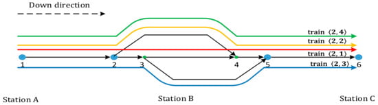
Figure 4.
Description about routing of trains of period-type 2.
For example, four trains of period-type 2 at station B, the routes of train includes arc (2, 3), arc (3, 4) and arc (4, 5), the routes of train and train both consist of arc (2, 4) and arc (4, 5), and regarding train , its routes covers arc (2, 3) and arc (3, 5). Thus, it can be seen that trains of the same period-type are allowed to choose different routes at the same station.
3.4. Definition for Integrated Routing and Scheduling of Multi-Periodic Trains
The problem of simultaneous multi-periodic train timetabling and routing takes some period-types of trains as an input and aims to optimize each train’s routes at each visited station, and the entering and leaving time on each visited arc. In other words, it needs to search travel paths for all trains from their origins to terminals, and meanwhile optimize the entering and leaving time on all visited arcs on the constructed directed graph.
Specifically, the input data of the problem of simultaneous multi-periodic train scheduling and routing covers three parts:
- (1)
- A rail network, which is denoted by the directed graph, consists of nodes and multiple types of arcs.
- (2)
- Trains of multiple period-types, whose visited stations, stops and operation period-lengths are pre-determined.
- (3)
- All required operation time parameters, such as the minimum safety arrival time interval and minimum safety departure time interval, minimum and maximum running time in each section, and minimum and maximum dwelling time at each station.
All symbols related to the rail network, trains of all period-types, etc. are introduced in Table 2.
Table 2.
All symbols for expressing the input data.
4. A Mixed Integer Linear Programming Model
4.1. Modeling Assumptions
The assumptions considered in our model are given in the following.
A1. All trains of one period-type travel through the sections of the line with the same running speed and have the same dwelling time at intermediate stations. However, all trains’ routes of a period-type are not the same.
A2. The number of period-types and trains are fixed and predetermined during the optimization of the multi-periodic train timetable and routes. Therefore, their optimization is not considered in our model.
A3. The period-length of each period-type is constant and cannot be changed, however, multiple period-types can have diverse period-lengths, that is, the period-lengths of different period-types can be same or different.
A4. The planning time is divided into one-minute time intervals. If required, it can be divided according to other shorter intervals, such as 30 or 15 s. Actually, the length of the time interval will not have any influence on our model in this paper. However, it may influence the scale and optimization efficiency of simultaneous multi-periodic train timetabling and routing.
4.2. Decision Variables
The decisions for each train include 1) the choice of each non-section arc, which constitutes each train’s travel path at its each visited station; 2) the entering time and leaving time on each visited arc; and 3) an auxiliary decision content, that is the sequence of two adjacent trains occupying the same visited arc, is required to describe the requirements of safety headways among trains’ arrivals and departures. Our decision-variables in this model are listed in Table 3.
Table 3.
Definition of decision-variables.
4.3. Objective of Minimizing the Total Travel Time of Trains
The objective of our model is minimizing the total travelling time of trains, that is, the travel-related time of all trains spent on each visited arc, including the operation time in each section and the dwelling time at each station, as follow.
Based on the leaving time and the entering time of train leaving off and entering arc , we compute the total travelling time-cost of all trains. For example, if the arc is a section arc, thus the represents operation time in the section arc , and if the arc is a station arc, thus the represents dwelling time-cost at this station arc . Finally, we sum up the time-cost of all trains spent on their visited arcs.
4.4. Constraints
The constraints considered in our model consist of the following eight groups.
Group I: Balanced constraints of trains at each station
Constraints (2) and (3) guarantee that each train can only choose one station arc to enter its each visited station, and only one station arc to leave. Constraint (4) sets balance of the inbound and outbound balance for each train at each intermediate node of each visited station.
Specifically, as shown in Figure 5, we assume that the station B is visited by train , thus as covered by constraint (2), can be arc (1,2) or (1,3). However, train can choose only one arc to enter the station B, so either or , as for constraint (3), can be arc (2,4) or (3,4). Yet, the train can only choose one arc to leave off the station B as well, so either or . Moreover, as for the intermediate node 2, the train can only choose arc (1,2) to enter the station, but it can only choose either arc (2,3) or (2,4) to leave it. Similarly, the intermediate node 3, it can only choose one station arc to enter and another station arc to leave. Note that station arcs of each station are clear; thus, a station arc can point out which station it belongs to.

Figure 5.
Station B consisting of four nodes.
Group II: Range constraints of trains’ entering time and leaving time on arcs
Constraints (5)–(8) guarantee that the entering time and leaving time of each train on its each visited arc must fall within the range of operation time, while the entering time and leaving time of each train on a non-visited arc should be 0. Specifically, constraints (5) and (6) ensure that if a train visits a station arc , then . Thus, its entering time and leaving time should be between 1 and ; otherwise, . Constraints (7) and (8) directly ensure that the entering time and leaving time of the train on each visited section arc should be between 1 and because it must visit each pre-determined section arc.
Group III: Constraints on departure time for each period-type’ first train at its origin
Constraint (9) makes sure that each period-type’ first train should depart from its origin station between its earliest departure time and latest departure time .
Group IV: Constraints of trains’ travelling time on each section arc and dwelling time on each arrival–departure track arc
Constraint (10) ensures that the travelling time of train on each section arc cannot be lower than the allowable minimum travelling time and cannot exceed the maximum travelling time . Constraint (11) guarantees that if a train visits a non-arrival–departure track arc , so , then its travelling time on this arc should fall between and .
Constraint (12) makes sure the dwelling time of each period-type’ first train on each arrival–departure track arc should be between and when this train visits this arc, then ; otherwise, the dwelling time of this trains on this arc should be 0.
Group V: Equality constraints of trains’ entering time and leaving time on neighboring arcs
Constraint (13) guarantees that the leaving time of train from the former arc is exactly equal to the time of this train entering the latter arc .
Group VI: Constraints on trains of the same period-type operating with an equal headway on each arrival–departure track arc
To make trains operate periodically and provide passengers with a disciplinary timetable, trains of the same period-type should enter and leave off each arrival–departure track arc with the same time interval and satisfy the following two constraints. The reason for making trains periodically operate on each arrival–departure track arc is that passengers must get on or get off a train on an arrival–departure track arc.
Constraint (14) ensures that the difference of entering time between train and train on the same visited arrival–departure track arc is equal to the period-length . Similarly, constraint (15) makes sure that the difference of leaving time between two trains on the same visited arrival–departure track arc should also be equal to the period-lengt .
Group VII: Headway constraints of leaving time and entering time among trains
The minimum safety time interval for trains entering section arcs from the same direction
The minimum safety time interval for trains leaving off section arcs from the same direction
The minimum safety time interval for trains occupying arcs except single section arcs
Constraint (16) ensures that for a section arc visited by both train and train , if train enters it after the train , , then the entering time interval of two trains cannot be less than the minimum, that is . Constraint (17) guarantees that the time interval their leaving time should satisfy the condition .
Constraint (18) guarantees the time interval of two trains occupying the same station arc from either the same direction or two opposite directions should be no less than the minimum safety time interval. To be specific, if trains and both visit a non-section arc , moreover, the train enter the arc after the train , thus and , then the time interval of the two trains occupying this arc should be no less than the minimum safety time interval . Note that the time of train entering the arc can be denoted as either or , while the time of train leaving off the arc can be denoted as either or . Constraint (19) makes sure that the time interval of two trains occupying the same two-way section arc from two opposite directions should be no less than the minimum safety time interval based on the fact that they must visit their section arcs.
Group VIII: Consistency constraints on sequence of trains occupying arcs
Constraints (20) and (21) ensure that if trains and both visit a station arc , then , thus the values of both and can be either 1 or 0; otherwise, they are both equal to 0. Constraint (22) makes sure that only one of them can be 1.
To explain why the constraint (12) only needs to guarantee the dwelling time of the first train of period-type on an arrival–departure track arc should be between and ; we introduce a lemma. The lemma proves that as long as the dwelling time of the first train of each period-type at each station locates in between its minimum and maximum, other trains of each period-type can implicitly satisfy such kind of requirement. The specific lemma and its proof are as follows.
Lemma 1.
As long as the dwelling time of each period-type’ first train at each station falls between its minimum and maximum, other trains of each period-type can implicitly satisfy such kind of requirement.
Proof .
Constraint (12) is only for each period-type’ first train as other trains of the same period-type can satisfy such kind of constraint under the combined action of constraints (12), (14), and (15). Specifically, according to constraints (14) and (15), we can obtain the following two equations:
Next, the dwelling time of all trains of period-type on each arrival–departure track arc is equal to the dwelling time of the first train of this period-type, shown as follows:
Thus, if each period-type’ first train satisfies constraint (12), the following inequality should also be satisfied.
Therefore, the inequality of other trains of this period-type can be established, as follow.
Finally, constraints of all trains’ dwelling time on each arrival–departure track arc can be satisfied.
□
5. A Strategy for Simplifying Model
In this chapter, in order to improve the efficiency of solving the model, a strategy will be designed to partly predetermine the sequence of trains occupying the same arrival-departure track. First, in Section 5.1, the required notations for describing the strategy are introduced, and the strategy itself will be presented in Section 5.2.
5.1. Description of Added Notations
To improve the solve efficiency and computation speed of our model, we add four notations to our model, as shown in Table 4.
Table 4.
Added notations for simplifying the model.
First, it needs to be noted that values of and are computed based on the earliest departure time of the first train of period-type w at its origin station, the latest departure time of the first train of period-type w at its origin station in Table 2, and their values are known in advance. Then, values of and can be calculated based on values of and , as shown below:
Thus, we will only describe the computational process of and . For more clarity and detail, we take the first train of period-type two. An example is shown in Figure 6.
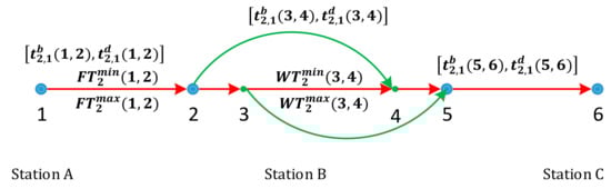
Figure 6.
Example of the first train of period-type two.
In Figure 6, the node 1 is an origin of train at station A, nodes 2, 3, 4, and 5 belong to station B, and node 5 is terminus of train at station C. Arcs (1, 2) and (5, 6) are section arcs, arcs (2, 3) and (4, 5) are non-arrival–departure track arcs, then arcs (2, 4), (3, 4), and (3, 5) are arrival–departure track arcs for trains dwelling at station B. Moreover, there is a hypothesis that arcs marked in red are visited by train , that is the train departs from station A, passes by arcs (1, 2) and (2, 3), selects arc (3, 4) to dwell at station B, then via arcs (4, 5) and (5, 6) arriving at station C.
Therefore, it is obvious that the earliest departure time of train at station A is and the latest departure time of train at this station is at station A, as trains of the same period-types should depart from their origin with an identical time interval. Then, the minimum and maximum running time on arc (1, 2) are and , and on arc (2,3) are and , thus the earliest and latest time of train entering arc (3, 4) can be computed, as follows:
After dwelling on arc (3, 4), the train should enter the arc (5, 6) in the time range of . Based on the minimum and maximum dwelling time of train are respectively and at station B, the earliest and latest time of train entering arc (5,6) can be computed, as follows:
5.2. The Simplified Strategy
The sequence of two trains entering an arc depends on their entering time, thus we can in advance find out the specific entering sequence of partly trains by comparing their earliest and latest entering time on an arc in advance, as shown in Section 5.1. Then, values of some can be predetermined, so that we can cancel some constraints that are satisfied automatically or simplify some constraints according to the predetermined values of .
For convenience, is defined as the th set for train on an arc . Therefore, for trains in , some parameters on the arc must satisfy the inequity in the set. Taking as an example, for each train belonging to set, its earliest entering time on the arc minus its latest entering time on the arc must be no less than the minimum safety time interval .
Then, based on the definition of , for trains in , some constraints can be cancelled or adjusted, being the simplified strategy for our model. The specific simplified process and descriptions are as follows.
As to the minimum safety time interval for trains entering a section arc from the same direction, constraint (16) is determined for each two trains using it. Apparently, because of the limitation of a train departure time at its origin, the entering time of each train on each arc is also limited. Thus, if the value difference value between the earliest entering time of train and the latest entering time of train on arc is no less than the minimum safety time interval , as shown in , and it is the same with trains in , then the constraint (16) has already been satisfied automatically. Therefore, constraint (16) in Group VII can be cancelled. On the other hand, if the difference value is no more than but is more than zero, thanks to the fact that the sequence of entering the arc is also known, as each train in enters the arc after train , then , thus constraint (16) can be adjusted as constraint (23) for simplification. While as for each train in , it enters the arc before train . Thus , so the constraint (16) can be ignored as it is sure to be satisfied.
As to the minimum safety time interval for trains leaving off a section arc from the same direction, constraint (17) is set for each two trains using it. Similarly, if the difference value between the latest leaving time of train and the earliest leaving time of train on arc is no less than the minimum safety leaving time interval , as shown in , it is also true for trains in , then the constraint (17) has also been satisfied automatically. Thus, constraint (17) in Group VII can be cancelled. Exception is the situation, where two trains do not belong to one of or , but as long as the earliest entering time of the train is no less than the latest entering time of the train , so , as shown in , then constraint (17) can be adjusted as constraint (24). However, as shown in , the train enters the arc before the train , then, , thus the constraint (17) can be ignored as it is sure to be satisfied.
As to the minimum safety time interval for trains occupying arcs except single section arcs, constraints (18) and (19) are still set for each two trains using it. Similarly, if the difference value between the earliest entering time of train and the latest leaving time of train on arc is no less than the minimum safety occupying time interval , as shown in . Then, the constraints (18) and (19) both have been satisfied automatically, thus they can be cancelled. It is the same with trains in . However, if the safety time interval has not been satisfied, the difference value is more than zero, then train enters the arc after train . Thus, , as shown in , thus constraints (18) and (19) can be adjusted as constraint (25). While trains in , , constraint (19) is sure to be satisfied.
As to the consistency constraints on sequence of trains occupying each arc, if we determine their specific sequence of entering each arc, then all constraints in Group VIII can be cancelled. As shown in , the latest entering time of train is no more than the earliest entering time of train on arc , it shows that the train enters the arc after the train , then , all constraints in Group VIII have been satisfied. It is the same with .
In conclusion, for better understanding, the cancelled or adjusted constraints for each are displayed in Table 5. For example, as for trains in , the constraint (16) can be cancelled, and as for trains in , the constraint (16) can be adjusted as constraint (23).
Table 5.
The cancelled or adjusted constraints for each .
6. Numerical Analysis
For this section, a small railway network consisting of eight stations is constructed, and numerous problem instances are solved to evaluate the performance, efficiency and stability of our proposed model in Section 6.1. Moreover, the influence of some main factors are also analyzed, such as the number of arrival–departure tracks at stations. Next, a more complicated problem on the Guangzhou–Zhuhai inter-city rail network is given to test the practicability of the model in Section 6.2.
6.1. Performance, Efficiency, and Stability Analysis on a Small Constructed Rail Network
6.1.1. Inputs and Parameters
In Figure 7, the rail network includes eight stations. Thus, there are seven sections, in which there are five one-way double-track sections and two two-way single-track sections. The three terminal stations are Station A, with four two-way arrival-departure tracks; Station F, with six two-way arrival–departure tracks; and Station H, with 5 two-way arrival–departure tracks. Junction Station C consists of four one-way arrival–departure tracks; intermediated Station B, D, and E correspond to 2, 2, and 4 one-way arrival–departure tracks; and intermediated Station G consists of three two-way arrival–departure tracks.
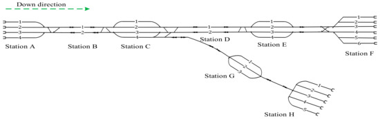
Figure 7.
A constructed railway network.
All trains on this railway network are classified into five period-types, and among them, trains of period-type 1–3 are from Station A to Station F, and trains of period-type 4 and 5 are from Station A to Station H. Their traverse and stop stations are shown in Table 6. Furthermore, the range of departure time of each period-type’s first train at its origin is also given in Table 6. In addition, all trains should operate between 06:00 and 15:00.
Table 6.
The specific input for each period-type.
Table 7 presents the allowed maximum and minimum time for trains running in each section, and Table 8 gives the maximum and minimum dwelling time of trains at each station. Note that, the running time at each station is set as 1 min for trains that do not dwell at it. Moreover, the minimum safety time intervals for trains entering and leaving off each section are set as three minutes and four minutes, respectively, and the minimum safety time interval occupying the same arrival–departure tracks at each station or each two-way section is two minutes.
Table 7.
The allowed maximum and minimum time for trains running in each section (minutes).
Table 8.
The allowed maximum and minimum time for trains dwelling at each station (minutes).
Based on the data given above, numerous problem instances are solved using WebSphere ILOG CPLEX (International Business Machines Corporation, New York, NY, USA) to evaluate the efficiency of the model and the simplified strategy, and they are all performed on a Lenovo C560 laptop (Lenovo Corporation, Beijing, China) with 3.2 GHz IntelICoreIi5 CPU with 8.0 GB of memory and a Windows 10 (Microsoft Corporation, Washington, DC, USA) 64-bit system.
6.1.2. The Benefits of Integrating Train Scheduling and Train Routing at Stations
To show the benefits of simultaneous train timetabling and routing, this section compares the results of either considering train routing or not. As long as the number of arrival–departure tracks at each station is large enough, such as 10 or 20 in our proposed model, then it poses the problem of train scheduling without the limitation of train routing.
In Figure 8, the left diagram gives the computational time and objective values under the two conditions of considering train routing and not. The right diagram presents the times that the number of trains occupying the same station at the same time is more than the number of usable arrival–departure tracks when not considering train routing as more than two trains occupy the same station at the same time do not exist when considering train routing. In it, V1 represents the number of trains occupying the same station at the same time minus the number of usable arrival–departure tracks is equal to one, and V2 represents the number of trains occupying the same station at the same time minus the number of usable arrival–departure tracks is larger than one. For example, in Figure 8, when the average number of trains of period-types is seven, the times of V1 is 12, that is the times that the number of trains occupying the same station minus number of usable arrival–departure tracks is equal to one is 12. Furthermore, for simplicity, use the “ANTP” to represent the average number of trains of period-types.
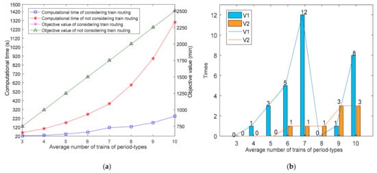
Figure 8.
(a) The computational time and objective values under the two conditions of considering train routing and not; (b) The times of two trains occupying the same station under the two conditions of considering train routing and not.
From the left diagram in Figure 8, we can see that the objective values under these two conditions of considering train routing or are not always the same with each other when the ANTP is increased from three to 10, but the computational time has a great difference. Because the computational time of considering train routing is from 23.66 s to 243.53 s, while it is from 59.31 s to 1300.41 s when not considering train routing; this causes their gaps to increase from 60.11% to 81.27%. However, from the right diagram, it is obvious that the times of V1 is increased until the ANTP is 7, and it is decreased when the ANTP is 8, that is because it first comes up the number of trains occupying the same station at the same time is three larger than the actual number of arrival–departure tracks at a station. After that, the total times of V2 is seriously increased to three times. Respectively, there are once and twice respectively that the number of trains occupying the same station at the same time is four and two larger than the actual number of arrival–departure tracks when the ANTP is 9, and 3. The times that the number of trains occupying the same station at the same time is two larger than the actual number of arrival–departure tracks when the ANTP is 10. Thus, a train timetable that does not integrate with train routes would not only take much computational time to obtain the optimal results, but also may gain an infeasible timetable when the number of trains occupying the same station at the same time is more than the number of usable arrival–departure tracks, and there may exist conflicts among trains at stations. An infeasible timetable would directly cause that some of trains cannot operate on time and indirectly decrease the operational efficiency of trains, thus increasing the waste of train capacity and energy consumption.
6.1.3. The Contribution of the Solving-Simplify Strategy to Solve Efficiency of Our Model
In order to analyze the contribution of the proposed strategy for improving the solve efficiency of our model, we are going to compare the objective values and computational time under the two conditions of considering train routing and not. To make it easier to describe, we use RS to represent the results optimized by the model added the simplified strategy, while R represents the optimal results obtained by the model not added the simplified strategy.
Based on the inputs and parameter settings in the Section 6.1.1, the compared results are shown in Figure 9. We calculate the percentage gap named Gap1 between their computational time for obtaining the RS and R by the Formula (26) and obtain their percentage gap called Gap2 of the number of constraints by the Formula (27).
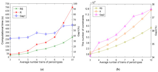
Figure 9.
(a) The comparison analysis of Gap1 between RS and R; (b) The comparison analysis of Gap2 between RS and R.
- CTR, CTRS are respectively computational time of R and RS.
- CONR, CONRS are respectively the number of constraints of R and RS.
In Figure 9, it shows that the objective values, computational time and number of constraints of RS and R all increase with improving ANTP, as more trains operate on the railway network, the number of constraints would increase, thus more computational time is needed to obtain the optimal timetable and trains’ routes at stations. Then, it is obvious that objective values of RS and R increase synchronously from 750 min to 2500 min, thus the simplified strategy would not change the optimal results. Nevertheless, it can reduce the number of constraints to some extent, as presented in the second diagram of Figure 9, the number of constraints of RS is increased from 8305 to 77,571, while that of R is from 12,602 to 124,350. This causes the gap between them to reach 37.62%. Thus, the computational time is increased from 39.15 s to 696.27 s when the ANTP is increased from 3 to 10, but that of RS is from 25.53 s to 279.88 s, and the Gap1 between them is increased from 34.80% to 59.80%. Moreover, it also seems that there is an upwards trend if we continue to increase the ANTP. In conclusion, the analysis indicates that the simplified strategy can really improve the solve efficiency of our model by reducing the number of constraints to obtain the same optimal results, moreover, the greater the ANTP is, the better the effect of improving the solve efficiency.
6.1.4. Performance and Stability Analysis of the Model
Because the performance and CT (Computational time) of our model are mainly influenced by the change of ANTP, the number of period-types, and simplified strategy. Thus, we will analyze them respectively in this sub-section.
- (1)
- Performance analysis with increasing the ANTP
Figure 10 gives the optimal results of objective values and the computational time, they all increase with increasing the ANTP from three to 10 when the number of period-types is increased from three to seven. Moreover, with increasing the number of period-types’, the objective values are all also increased when the ANTP is increased from three to 10. Except that, it is obvious that the computational time has a slow increasing trend when the number of period-types are 3, 4, and 5, and it is much faster when the number of period-types are six and seven, especially when the ANTP is nine and 10, it increases rapidly, from 310.55 s to 938.11 s, and from 412.51 s to 1542.15 s corresponding to the number of period-types is six and seven.
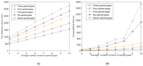
Figure 10.
(a) The variation tendency of objective values; (b) The variation tendency of computational time.
Figure 11 further gives the travel time of each single train of period-type one to seven. It can be seen that the travel time of a single train of each period-type always remains unchanged, although the ANTP has been increased to 10. Thus, increasing the ANTP would not change the travel time of a single train of each period-type, and this the reason why the objective value (the total travel time of trains) has been improved is that the number of trains on the railway network has been increased. Thus, the computational time should also be increased. Therefore, a multi-periodic timetable has a higher stability, and increasing or decreasing the number of trains of a certain period-type has a little influence on the current operational trains. This proves that it has high quality and is convenient for adjustment to improve the work efficiency of railway staff and reduce the waste of human resources.
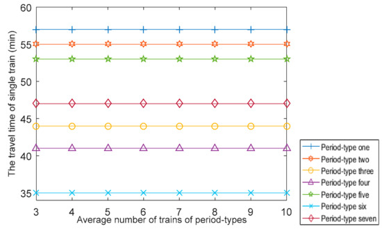
Figure 11.
The travel time of single train of each period-type.
- (2)
- Performance analysis with increasing the number of period-types
Here, we increase the number of period-types for trains of period-type one to analyze the influence of changing the number of period-types on the performance of our model. Therefore, we will divide trains of period-type one into one to 10 different period-types when the ANTP is increased from three to 10, but their stop plans and period-lengths remain unchanged. However, the range of departure time of each period-type’s first train at its origin should be increased based on the initial period-length of period-type one to make the departure time range of each train is same with it is in the same period-type. The specific number of period-types divided for trains of period-type one is presented in Table 9.
Table 9.
The number of period-types divided for trains of period-type one.
From the optimal results with increasing the number of period-types for trains of period-type one from one to 10, we obtain that their objective values and the travel time of a single train in each period-type are same with each other, while the number of constraints has been increased, therefore, the computational time increases, too. Figure 12 gives the number of constraints with increasing the NPT from 1 to 10 when the ANTP is increased from 3 to 10. As revealed in this figure, the number of constraints is always increasing slightly from NPT=1 to NPT=10 when the ANTP is increased from three to 10. Therefore, improving NPT will cause the number of constraints to increase in the process of train timetabling and routing. This will further increase the computational time to solve the problem, as shown in Figure 13.
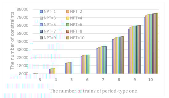
Figure 12.
The number of constraints with increasing the number of period-types.
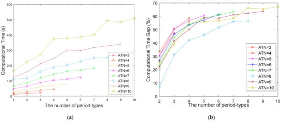
Figure 13.
(a) The variation tendency of computational time; (b) The variation tendency of the Gap of computational time.
In Figure 13, it is obvious that the computational time is improved with increasing NPT, its maximum is 509.75 s when NPT is increased to 10. Moreover, all computational time gaps are also increased with increasing NPT when NPT are two and three, most of gaps are between 30–50%, and when NPT are 4, 5, and 6, they are almost in 50–60%, while after that, most of gaps are between 60–70%, among them, the maximum is 67.2% when NPT is 10 when the ANTP is 10. Finally, although increasing the ANTP would not change the objective value, it would cause the computational time to increase greatly, thus the ANTP and the number of trains of each period-type should be arranged reasonably to better improve solve efficiency. Moreover, the computational time has an upward trend with increasing the number of period-types. This suggests that a multi-periodic train timetable with reasonable ANTP and reasonable number of trains of each period-type can make train scheduling more efficient.
- (3)
- Stability analysis of the simplified strategy with changing running time or dwelling time
To prove the stability of simplified strategy in decreasing the computational time to improve the solve efficiency of our model, we design eight instances with changing the maximum and minimum running time of trains in sections, and the maximum and minimum dwelling time of trains at stations, as they all are the main factors to influence the simplified strategy. First, we classify the eight instances into two categories:
- ■
- Category 1: Contracting the running time range in sections and dwelling time range at stations by decreasing their maximum or increasing their minimum.
- ■
- Category 2: Expanding the running time range in sections and dwelling time range at stations by increasing their maximum or decreasing their minimum.
In each category, there are four instances with changing maximum or minimum, whose specific characteristics are given in the Table 10. Note that, “+2, +1” represent the maximum or minimum are increased by two minutes, one minute respectively, “−2, −1” represent the maximum or minimum are decreased by two minutes, one minute respectively, while “—” represents the maximum or minimum remain unchanged. Except that, the maximum can only reduce to its minimum, while the minimum can be added to its maximum.
Table 10.
The specific characteristics of test problems.
By adjusting the inputs of model based on Table 10, we finally obtain the objective values of RS and R in the instances 1–8 when the ANTP is increased from 3 to 10. From the optimal results shown in Figure 14, we can discover that all objective values are the same compared with the optimal results of RS and R in the instances 1, 2, 5, and 6 when the maximum of running and dwelling time are changed. However, they are increased in instances 3 and 4 when the minimum of running and dwelling time is added. While they are decreased in the instances 7 and 8 corresponding to reducing the minimum of running and dwelling time. However, no matter how the objective values change, the all objective values in the eight instances of RS are the same with that of R. Therefore, reducing the minimum of running and dwelling time can slightly decrease the objective values, and adding the minimum of running and dwelling time will increase the objective values, while changing their maximum does not influence the objective values. This indicates that the simplified strategy has good stability.
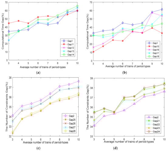
Figure 14.
The stability analysis diagrams of simplified strategy by the eight test problems. (a) The gaps of computational time of RS and R in instances 1–4; (b) The gaps of computational time of RS and R in instances 5–8; (c) The gaps of the number of constraints of RS and R in instances 1–4; (d) The gaps of the number of constraints of RS and R in instances 5–8.
To analyze comparatively, the (a) and (b) diagrams in Figure 14 give the gaps of computational time of RS and R in instances 1–8, and they are represented by the Gap11 to Gap18, moreover, the computational time of an infeasible solution is its upper band. Then the (c) and (d) diagrams in Figure 14 present the gaps of the number of constraints of RS and R in the test instances 1–8, and they are denoted by the Gap21 to Gap28. The Gap1 and Gap2 are the results in Figure 9. It can be known that most of gaps of computational time and the number of constraints increase when ANTP is added from three to 10 in instances 1–8. Thus, the simplified strategy has a good stability in improving the solve efficiency by reducing the number of constraints. In addition, Gap11 to Gap14 and Gap21 to Gap24 are, respectively, the gaps of computational time and the number of constraints in the category 1, while Gap15 to Gap18 and Gap25 to Gap28 are in category 2. By comparing their results with Gap1 and Gap2, we can discover that most of Gap11 to Gap14 are higher than Gap1, and all Gap21 to Gap24 are higher than Gap2, while all Gap15 to Gap18 are lower than Gap1, and all Gap25 to Gap28 are less than Gap2. Therefore, contracting the range of running time of trains in sections and the dwelling time of trains at stations can strengthen the impact of simplified strategy to further improve the solve efficiency of model, while expanding their range will cut down its effect of simplified strategy, moreover, it still can reduce the number of constraints to shorten the computational time as the gaps in instances 1–8 are all more than 0.
6.2. Application Analysis Based on the Guang-Zhu Inter-City Rail
In this section, a reality Guang-Zhu inter-city rail is devoted to evaluating the practicability of our proposed model. This inter-city railway totally includes 22 operating stations with different numbers of one-way and two-way arrival–departure tracks, as well as 21 operating one-way sections for up and down directions, respectively. Its main line is from Guangzhou South Station to Zhu-hai Station via 15 operation stations, such as Shun-de Station, Xiao-lan Station, and Zhong-shan Station, while its branch line is from Xiao-lan Station on the main line to Xin-hui Station, including Gu-zhen Station, Jiang-hai Station, Jiang-men Station, and Li-yue Station. Moreover, the length of the main line and the branch line is 151 km and 26 km respectively, as shown in Figure 15. This inter-city rail mainly serves for the large and rapid traffic travel demand in the economic circle of Zhu-hai, Zhong-shan, and Jiang-men, and located on the west bank of the Pearl River. Thus, it is an important part in the planning of the Pearl River Delta Railway.
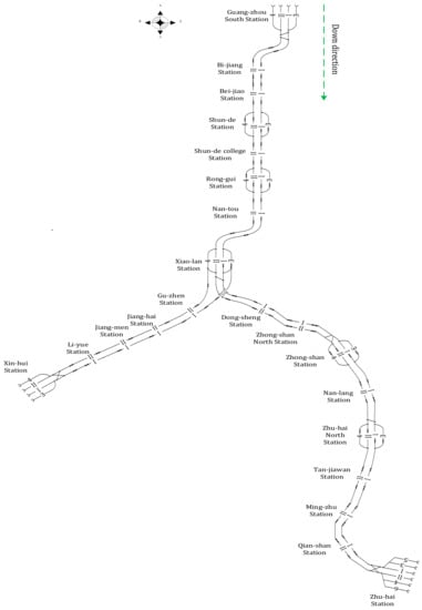
Figure 15.
The Guang-Zhu inter-city railway network.
At present, a total of 32 trains operate from Guangzhou South Station to Zhu-hai Station, while 21 trains are from Guangzhou South Station to Xin-hui Station. With the given number of trains and their stops, this paper divides these trains into seven period-types to analyze the problem of multi-periodic train timetabling and routing. Table 11 gives the more detailed information, such as the number of trains of each period-type, and their sequence of stop stations. Then, the maximum and minimum running time in each section and the maximum and minimum dwelling time at each station are presented in the Table 12 and Table 13.
Table 11.
The number of trains of each period-type and their stop stations.
Table 12.
The maximum and minimum running time in each section (minutes).
Table 13.
The maximum and minimum dwelling time at stations (minutes).
Table 14 gives the optimal results of RS and R, including objective values, computational time and the number of constraints. From the table, we can discover the objective values of RS and R are the same with each other, while the computational time and the number of constraints of R are much more than RS; thus, the Gap1 reaches 44.23%, while the Gap2 reaches 35.17%. This further proves the simplified strategy can improve the solve efficiency of the model.
Table 14.
Results of objective value, computational time and the number of constraints.
Table 15 shows some more detailed optimal results, including the departure time of each period-type’s first and last trains at origin stations, as well as each train’s travel time in sections and dwelling time at stations. Because trains of a period-type enter and leave each visited station with an identical time interval, the travel time of trains of the same period-type should be equal. From this table, we can obtain that the difference value of departure time at the origin station between the first and last train of the same period-type is equal to , that is,
This is exactly the regularity of the multi-periodic trains.
Table 15.
More detailed optimal results of each period-type.
To show the obtained multi-periodic train timetable and each train’s routes at its each visited station more clearly, Figure 16 gives the entering time and leaving time of trains of each period-type at their specific visited arrival–departure tracks. In this figure, arrival–departure tracks at each station are represented by the lines corresponding to this station. For example, the four lines corresponding to Guangzhou South station respectively represent the four arrival–departure track in sequence, thus we can know easily each arrival–departure track’s occupation information, including train’s identification and its entering time, dwelling time and leaving time. For example, train ⟨1, 1⟩ enters the Shun-de station at 06:32 occupying the first arrival–departure track for four minutes, then leaves off this station at 06:36. In addition, there are some regularities worth noting in this figure.
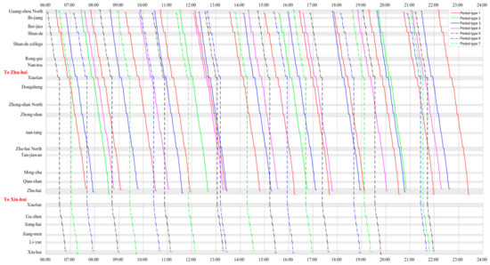
Figure 16.
The time of trains of each period-types entering and leaving off the specific arrival–departure tracks at each visited station.
- (1)
- Trains of the same period-type have the same stop plan, enter and leave off each visited station with the same period-length to make the train timetable more regular. Thus, it can provide convenience for passengers, attract more passengers, and achieve good social and economic benefits for the high-speed railway. Moreover, this kind of regularity can also improve the efficiency of transportation organization on a high-speed railway network. Moreover, the trains’ chosen arrival–departure tracks at each visited station can be different so as to realize the efficient allocation of traffic resources on a high-speed railway.
- (2)
- The running time of trains of each period-type almost cross the whole operation time to meet passenger demand over the day, and the strict period-length ensures the regularities of multi-periodic trains to provide convenience for passengers. Furthermore, the number of trains of each period-type may be different according to changes in passenger demand. For example, it needs to operate 12 trains in the period-type 1, the first train’s departure time is 06:25, and the last train’s arrival time is 23:24, while it only needs to operate four trains in the period-type 2, the first train’s departure time is 07:27, and the last train’s arrival time is 20:50.
7. Conclusions and Further Studies
In order to avoid conflicts of trains at stations and obtain a feasible timetable, and provide passengers with a regular train timetable, this paper is committed to studying the problem of multi-periodic train timetabling and routing at stations on a high-speed rail network. This problem aims to not only arrange the routes of trains at each visited station but also make them enter and leave each arrival–departure track with the same headway. Our conclusions of this paper are as follows.
- (1)
- Based on a large number of numerical examples, it is obvious that our proposed mixed integer linear programming model has good performance, stability, and practicability in solving the problem of simultaneous multi-periodic train timetabling and routing.
- (2)
- The simplified strategy in our model can greatly reduce the computational time by 30–50%, so as to improve the solve efficiency by reducing the number of constraints, and it is also proved that it has a good stability by changing its main impact factors. Moreover, the more trains that operate, the more obvious the effect is.
- (3)
- Train timetables that consider trains’ routes at stations can eliminate conflicts among trains at stations to improve the efficiency of trains’ operating. It is especially obvious with increasing the number of trains. For example, in Figure 8, when the ATNP is 6, it first occurs when more than two trains conflicts at the same station. When the ATNP is 7, the times of conflicts reached more than 13.
- (4)
- Compared with an aperiodic train timetable, a multi-periodic train timetable has higher computation efficiency that can be improved from 30% to 67.2% with increasing the number of period-types. In addition, trains’ operating density on a multi-periodic train timetable can better satisfy the time-varying of passenger demand to provide better service for passengers on a high-speed rail network.
In conclusion, train timetables that consider trains’ routes at stations can improve the operational efficiency of trains. Furthermore, the regular and fixed departure and arrival time of trains are convenient for passengers to remember so as to provide convenience for them. All of the above features contribute to the appeal of high-speed railway, thus strengthening its sustainable development. Due to the elimination of conflicts among trains at stations, this can improve the efficiency of management, reduce the waste of human resource, and improve the operation efficiency of railway systems. Once a conflict happens, the operator will need to arrange for additional workers to handle it. This is a waste of time and human resources. Moreover, a multi-periodic train timetable is beneficial to improve the efficiency of transportation organization and management for the higher computation efficiency. Practically, it also simplifies the management and adjustment of trains for its regularity. For example, as for the decrease of passenger demand in some non-peak hours, a multi-periodic train timetable can stop some trains of a certain period-type, and it will not have any influence on other trains. Thus, a multi-periodic train timetable is more conducive to the management of transportation systems.
Our further studies on this research will mainly focus on the following three aspects.
- (1)
- Take more practical factors in the process of train operating into account, such as acceleration, deceleration, and dwelling of trains in the sections, so that the obtained train timetable is more feasible when applied to the real-world situations. Moreover, the robustness of a train timetable should also be considered to cope with possible delays or disturbances.
- (2)
- To consider the distribution of passenger demand in the process of the multi-periodic train timetabling and routing so as to design a train timetable that can match with the change of passenger demand. Some indicators related with passenger service level can also be added. Moreover, based on the change of passenger demand, we can adjust the stop plan of trains to reduce the unnecessary stops of trains and unnecessary usage of arrival–departure tracks at stations.
- (3)
- The optimization of periodic and non-periodic train timetabling or routing on a high-speed rail network. While most trains are arranged to run with a fixed regular interval, some non-periodic trains are allowed to operate at some time-periods with higher passenger demand.
In this way, the obtained train timetable may be able to better adapt to fluctuation of passenger demand at different time-periods during the whole day.
Author Contributions
W.Z. and X.Y. conceived the research, built the models and proposed the simplified strategy; X.Y. wrote the matlab program and carried out the instance experiments; X.Y. and W.F. conducted data analysis based on the results of the instance experiments; W.Z. and X.Y. were responsible for writing the paper; and W.Z., and W.F. assisted in revising the paper. All authors have read and agreed to the published version of the manuscript.
Funding
This study work was partially funded by the National Natural Science Foundation of China (Grant No. U1934216, 71871226, U1834209), the Natural Science Foundation of Hunan Province, China (Grant No. 2018JJ3698), and the Fundament Research Funds for the Central Universities of Central South University (Grant No. 2019zzts546). The authors are responsible for all conclusions and opinions in this paper.
Acknowledgments
The authors would like to express great appreciation to editors and reviewers for their positive and constructive comments.
Conflicts of Interest
The authors declare no conflict of interest.
References
- Mu, S.; Dessouky, M. Efficient dispatching rules on double tracks with heterogeneous train traffic. Transp. Res. Part B Methodol. 2013, 51, 45–64. [Google Scholar] [CrossRef]
- Cai, X.; Goh, C. A fast heuristic for the train scheduling problem. Comput. Oper. Res. 1994, 21, 499–510. [Google Scholar] [CrossRef]
- Caprara, A.; Fischetti, M.; Toth, P. Modeling and Solving the Train Timetabling Problem. Oper. Res. 2002, 50, 851–861. [Google Scholar] [CrossRef]
- Caimi, G.; Chudak, F.; Fuchsberger, M.; Laumanns, M.; Zenklusen, R. A New Resource-Constrained Multicommodity Flow Model for Conflict-Free Train Routing and Scheduling. Transp. Sci. 2011, 45, 212–227. [Google Scholar] [CrossRef]
- Pellegrini, P.; Marlière, G.; Rodriguez, J. Optimal train routing and scheduling for managing traffic perturbations in complex junctions. Transp. Res. Part B Methodol. 2014, 59, 58–80. [Google Scholar] [CrossRef]
- Xu, X.; Li, K.; Yang, L. Scheduling heterogeneous train traffic on double tracks with efficient dispatching rules. Transp. Res. Part B Methodol. 2015, 78, 364–384. [Google Scholar] [CrossRef]
- Sparing, D.; Goverde, R.M.P. A cycle time optimization model for generating stable periodic railway timetables. Transp. Res. Part B Methodol. 2017, 98, 198–223. [Google Scholar] [CrossRef]
- Odijk, M.A. A constraint generation algorithm for the construction of periodic railway timetables. Transp. Res. Part B Methodol. 1996, 30, 455–464. [Google Scholar] [CrossRef]
- Zhou, W.; Yang, X. Timetable Optimization for High-Speed Rail with Multiple Operating Periods: Solving Method Based on a Framework of Lagrangian Relaxation Decomposition. Transp. Res. Rec. J. Transp. Res. Board 2016, 2546, 43–52. [Google Scholar] [CrossRef]
- Zhou, W.; Tian, J.; Xue, L.; Jiang, M.; Deng, L.; Qin, J. Multi-periodic train timetabling using a period-type-based Lagrangian relaxation decomposition. Transp. Res. Part B Methodol. 2017, 105, 144–173. [Google Scholar] [CrossRef]
- Samà, M.; D’Ariano, A.; Pacciarelli, D.; Corman, F. Lower and upper bound algorithms for the real-time train scheduling and routing problem in a railway network. IFAC-PapersOnLine 2016, 49, 215–220. [Google Scholar] [CrossRef]
- Mees, A. Railway scheduling by network optimization. Math. Comput. Model. 1991, 15, 33–42. [Google Scholar] [CrossRef]
- Törnquist, J.; Persson, J.A. N-tracked railway traffic re-scheduling during disturbances. Transp. Res. Part B Methodol. 2007, 41, 342–362. [Google Scholar] [CrossRef]
- Szpigel, B. Optimal train scheduling on a single track railway. Oper. Res. 1972, 72, 343–352. [Google Scholar]
- D’Ariano, A.; Pacciarelli, D.; Pranzo, M. A branch and bound algorithm for scheduling trains in a railway network. Eur. J. Oper. Res. 2007, 183, 643–657. [Google Scholar] [CrossRef]
- Dessouky, M.M.; Lu, Q.; Zhao, J.; Leachman, R.C. An exact solution procedure to determine the optimal dispatching times for complex rail networks. IIE Trans. 2006, 38, 141–152. [Google Scholar] [CrossRef]
- Cardillo, D.D.L.; Mione, N. k L-list λ colouring of graphs. Eur. J. Oper. Res. 1998, 106, 160–164. [Google Scholar] [CrossRef]
- Zwaneveld, P.J.; Kroon, L.G.; Van Hoesel, S.P. Routing trains through a railway station based on a node packing model. Eur. J. Oper. Res. 2001, 128, 14–33. [Google Scholar] [CrossRef]
- Caimi, G.; Burkolter, D.; Herrmann, T. Finding Delay-Tolerant Train Routings through Stations. Oper. Res. Proc. 2005, 2004, 136–143. [Google Scholar]
- Lusby, R.M.; Larsen, J.; Ehrgott, M.; David, R. Railway track allocation: Models and methods. OR Spectr. 2011, 33, 843–883. [Google Scholar] [CrossRef]
- Billionnet, A. Using Integer Programming to Solve the Train-Platforming Problem. Transp. Sci. 2003, 37, 213–222. [Google Scholar] [CrossRef]
- Goverde, R.M.; Hansen, I.A. Performance indicators for railway timetables. In Proceedings of the IEEE International Conference on Intelligent Rail Transportation (ICIRT), Beijing, China, 30 August–1 September 2013; pp. 301–306. [Google Scholar]
- Burggraeve, S.; Vansteenwegen, P. Robust routing and timetabling in complex railway stations. Transp. Res. Part B Methodol. 2017, 101, 228–244. [Google Scholar] [CrossRef]
- Mazzarello, M.; Ottaviani, E. A traffic management system for real-time traffic optimisation in railways. Transp. Res. Part B Methodol. 2007, 41, 246–274. [Google Scholar] [CrossRef]
- Dewilde, T.; Sels, P.; Cattrysse, D.; Vansteenwegen, P. Robust railway stationplanning: An interaction between routing, timetabling and platforming. J. Rail Transp. Plan. Manag. 2013, 3, 68–77. [Google Scholar]
- Lee, Y.; Chen, C.Y. A heuristic for the train pathing and timetabling problem. Transp. Res. Part B Methodol. 2009, 43, 837–851. [Google Scholar] [CrossRef]
- Castillo, E.; Gallego, I.; Ureña, J.M.; Coronado, J.M. Timetabling optimization of a mixed double- and single-tracked railway network. Appl. Math. Model. 2011, 35, 859–878. [Google Scholar] [CrossRef]
- Morlok, E.K.; Peterson, R.B. Final report on a development of a geographic transportation network generation and evaluation model. Transp. Res. Forum. 1996, 90, 26–44. [Google Scholar]
- Li, F.; Gao, Z.; Li, K.; David, Z.; Wang, W. Train Routing Model and Algorithm Combined with Train Scheduling. J. Transp. Eng. 2013, 139, 81–91. [Google Scholar] [CrossRef]
- Zhou, W.; Teng, H. Simultaneous passenger train routing and timetabling using an efficient train-based Lagrangian relaxation decomposition. Transp. Res. Part B Methodol. 2016, 94, 409–439. [Google Scholar] [CrossRef]
- Wardman, M.; Shires, J.; Lythgoe, W.; Tyler, J. Consumer benefits and demand impacts of regular train timetables. Int. J. Transp. Manag. 2004, 2, 39–49. [Google Scholar] [CrossRef]
- Johnson, D.; Shires, J.; Nash, C.; Tyler, J. Forecasting and appraising the impact of a regular interval timetable. Transp. Policy 2006, 13, 349–366. [Google Scholar] [CrossRef]
- Serafini, P.; Ukovich, W. A Mathematical Model for Periodic Scheduling Problems. SIAM J. Discret. Math. 1989, 2, 550–581. [Google Scholar] [CrossRef]
- Goverde, R.M.P. Improving Punctuality and Transfer Reliability by Railway Timetable Optimization; Delft University Press: Delft, The Netherlands, 1999. [Google Scholar]
- Kroon, L.G.; Peeters, L.W.P. A Variable Trip Time Model for Cyclic Railway Timetabling. Transp. Sci. 2003, 37, 198–212. [Google Scholar] [CrossRef]
- Lindner, T. Train Schedule Optimization in Public Rail Transport. Ph.D. Thesis, Technische Universität Braunschweig, Braunschweig, Germany, 2000. [Google Scholar]
- Heydar, M.; Petering, M.E.; Bergmann, D.R. Mixed integer programming for minimizing the period of a cyclic railway timetable for a single track with two train types. Comput. Ind. Eng. 2013, 66, 171–185. [Google Scholar] [CrossRef]
- Nachtigall, K.; Voget, S. A genetic algorithm approach to periodic railway synchronization. Comput. Oper. Res. 1996, 23, 453–463. [Google Scholar] [CrossRef]
- Sels, P.; Cattrysse, D.; Vansteenwegen, P. Automated platforming & routing of trains in all Belgian railway stations. Expert Syst. Appl. 2016, 62, 302–316. [Google Scholar]
- Nachtigall, K. Periodic network optimization with different arc frequencies. Discret. Appl. Math. 1996, 69, 1–17. [Google Scholar] [CrossRef]


© 2020 by the authors. Licensee MDPI, Basel, Switzerland. This article is an open access article distributed under the terms and conditions of the Creative Commons Attribution (CC BY) license (http://creativecommons.org/licenses/by/4.0/).