Article

Impact of Climate Extremes on Suitability Dynamics for Japanese Scallop Aquaculture in Shandong, China and Funka Bay, Japan

1
Lab. of Fisheries Oceanography, College of Fisheries, Ocean University of China, Qingdao 266003, China
2
Institute for Advanced Ocean Study, Ocean University of China, Qingdao 266100, China
3
Arctic Research Center, Hokkaido University, N21 W11 Kita-Ku, Sapporo 001-0021, Japan
4
PASCO Research Institute, PASCO Corporation, Tokyo 153-0043, Japan
*
Authors to whom correspondence should be addressed.
Sustainability 2020, 12(3), 833; https://doi.org/10.3390/su12030833
Submission received: 1 December 2019 / Revised: 8 January 2020 / Accepted: 9 January 2020 / Published: 22 January 2020
(This article belongs to the Section Sustainable Agriculture)

Abstract

:
The assessment of extreme weather events on suitable sites for aquaculture could help in establishing sustainable coastal environmental resource management. Japanese scallop culture is an economically important marine farming activity in the coastal communities of Shandong, China and Funka Bay, Japan. In this study, we improved the suitable aquaculture site-selection model (SASSM) by using Geostationary Ocean Color Imager (GOCI) data instead of Moderate Resolution Imaging Spectroradiometer (MODIS) data, as a complementary source for higher temporal and spatial resolution data that are useful for monitoring fine-scale coastal and oceanic processes. We also applied the newly developed SASSM to the Japanese scallop production site along the Shandong coast. Finally, we analyzed the correlations between environmental factors (chlorophyll a concentration, sea surface temperature (SST), and total suspended sediment), meteorological factors (precipitation, temperature, and wind), and climatic events (winter East Asian monsoon (EAM) and El Niño/La Niña Southern Oscillation), and the impacts of climate events on suitable zones for scallop aquaculture. The new SASSM maps show that GOCI products have the potential for oceanographic investigations in Shandong, China and Funka Bay, Japan. Our results highlighted higher aquaculture site suitability for scallop in Funka Bay than in Shandong coast. During the winter with a strong EAM (2011), the suitable area for Japanese scallop aquaculture increased. Conversely, in the winter during a strong El Niño (2016), we found fewer areas that were highly suitable for scallop aquaculture in Funka Bay. SST was extremely low in Funka Bay during spring and summer 2017, which caused fewer highly suitable areas (scores of 7 and 8) for scallop aquaculture relative to other years. These findings suggest that extreme climatic events significantly impact the availability of suitable sites for marine farming and thus, should be considered in the development and design of coastal aquaculture sites.

1. Introduction

In recent years, an increase in the intensity and frequency of extreme weather events has been reported [1]. For example, in the winter of 2010, East Asia, Europe, and North America suffered from extremely cold weather [2]. According to monitoring reports by NOAA (National Oceanic and Atmospheric Administration) Climate prediction center, the 2015/2016 El Niño was one of the strongest El Niño events in the past twenty years [3]. The sea surface temperature in the Yakumo coastal region, Hokkaido was reported to be extremely cold in 2017 summer. These extreme events are rare, although they may become more common in the future, as a result of climate variability [4]. Climate extremes have serious impacts on coastal ecosystems, where they have affected the stability of human food sources, limiting adequate nutrition and therefore sustainable social and economic development [5,6,7]. However, there are few studies on the impact of climate extremes on the aquaculture environment.
Worldwide, aquaculture production accounted for 46.8% of total fish production from capture fisheries and aquaculture in 2016 [8]. Total aquaculture production in China and Japan were 49,244 and 677 thousand tonnes that year, accounting for 61.5% and 0.8% of global production, respectively. China maintains the largest share of global fish production from aquaculture by far [8]. Among aquaculture species, scallops offer high yield, high nutritional value, and economical production, and thus have been favored by the aquaculture industry. The Japanese scallop, native to the Funka Bay of Japan, was first introduced to China in 1982 for aquaculture, where it quickly became a popular shellfish. It has been widely promoted and cultivated in the Northeast Shandong coastal area [9]. Since 2000, the worldwide annual production of Japanese scallops has stabilized at 1.1–1.2 million tonnes [8], with China and Japan being the major producers.
In recent years, with increased regional climate variability, the growth and yield of Japanese scallops in Funka Bay and Shandong coastal waters have undergone fluctuations [6,10]. Therefore, it is critical to establish a precise and scientific marine resource management method for the sustainable development of aquaculture areas. In this work, we implemented an approach that not only estimates suitable sites available for cultured species but also evaluates responses of marine living resources to combined impacts of climate and environmental changes. Thus, providing decision support systems for integrated management of aquaculture activities is expected.
Satellite remote sensing and geographic information system (GIS) technology, developed over the past three decades, are powerful tools and platform immensely useful across research disciplines [11]. Satellite remote sensing, in particular, has a wide range of short-term, low-cost features such as real-time analysis of synoptic and high-precision environmental data over large temporal and spatial scales. In the marine environment, GIS can provide a visual interface, data modeling tools, and other statistical functions [12]. Therefore, remote sensing and GIS technology present broad applicability in marine fisheries resource assessment and fisheries management research. Several studies have used Moderate Resolution Imaging Spectroradiometer (MODIS) data and GIS technology to develop suitable aquaculture site selection models (SASSMs) in Funka Bay [13,14,15]; these SASSMs have been extended to the Dalian area [6,10]. However, as the service life of MODIS ends, an alternative source of satellite remote sensing data is needed for this approach. The world’s first geostationary satellite-based ocean color sensor, Geostationary Ocean Color Imager (GOCI) was launched on June 27, 2010 from South Korea; this sensor covers the Japanese scallop aquaculture regions in China and Japan. GOCI has an hourly repeat cycle and 500-m spatial resolution [16], which could provide valuable information for marine environmental studies and evaluation of marine resource models.
The objectives of this study were to (1) evaluate and compare GOCI and MODIS data and discuss the feasibility of replacing MODIS with GOCI in SASSMs, (2) improve SASSMs by employing GOCI data in the Funka Bay and newly-developed SASSM to Shandong coastal region for Japanese scallop aquaculture, and (3) examine the potential impacts of climate extremes on the development of Japanese scallop aquaculture in the Shandong coastal region and Funka Bay.

2. Materials and Methods

2.1. Scallop Culture in Study Area

Shandong is a coastal province at the eastern margin of the North China Plain along the lower reaches of the Yellow River, and is rich in marine resources. Its offshore area makes up 37% of the total area of the Bohai and Yellow Seas, with a shoal area accounting for 15% of the China’s total (Figure 1). Aquaculture in Shandong leads the country in the production of prawns, bivalves, abalones, sea slugs, and urchins in China. The production of marine scallop aquaculture in Shandong was 761,000 tonnes in 2014, which accounted for 47% of the China’s total [17].
Funka Bay is located in the coastal waters of southern Hokkaido in northern Japan, a region affected by the inflow of warm Tsugaru water from autumn to winter and cold Oyashio water from spring to summer [18]. Scallop aquaculture industry can be found all along the coast of Funka Bay. The annual production of cultured Japanese scallops in Funka Bay was approximately 123,954 tonnes in 2015 and the value of Japanese scallops in Funka Bay was 2929 million JPY in 2015 [19]. Annual scallop production data per region (Figure 2) are published by the Fisheries Department of the Hokkaido government and are available at the Marinenet Hokkaido website [19]. The annual scallop production of Yakumo accounts for about 30% of total Funka bay region. Scallop aquaculture uses suspension culture in both Shandong and Funka Bay region.

2.2. Data Used and Processing

2.2.1. MODIS and GOCI Data

The marine environmental factors examined include SST, chlorophyll a (Chl-a) concentration, and total suspended sediment (TSS) concentration, which were derived from MODIS (Moderate Resolution Imaging Spectroradiometer)-Aqua (a spacecraft launched on May 4, 2002 by NASA, Washington, DC). reprocessing R2018.0 (2014.0 for SST) (provided by NOAA, Washington, DC, USA) as Level 2 data with 1-km resolution. All daily Level 2 Ocean Color (OC) and SST (11 um) data from 1 April 2011 to 30 July 2018 were downloaded from the Ocean Color website and processed using SeaDAS v7.5 (NOAA, Washington, DC, USA) [20]. Level 2 to Level 3 processing entails mapping data from the raw satellite perspective to cylindrical coordinates. The first step is to spatially bin the file (l2 bin “binary”), and then creating temporal average for monthly observation (l3 bin), and finally create a mapped l3 bin data (l3 mapgen “map generation”) and write it as a 2D floating point array of the geophysical data with 1 km spatial resolution. Monthly-average nLw (555) images were used to calculate TSS concentration images (g m-3) based on Ahn’s algorithm [21], where nLw (555) is normalized water leaving radiance at 555 nm, serving as an indicator of water column turbidity.
We acquired all daily GOCI (Geostationary Ocean Color Imager) L1B data from 1 April 2011 to 30 July 2018 from the Korea Ocean Satellite Center (KOSC) website [22]. GOCI L1B data were processed through the standard GOCI Data Processing System software (GDPS v2.0) (Korea Institute of Ocean Science and Technology (KIOST), Busan, Korea) to produce Level 2 products using default atmospheric correction [16] for Chl-a and TSS data. Shandong coastal water is more turbid than Funka Bay, therefore the Yoc [23] and OC2 [24] algorithms were used for Chl-a concentration and TSS processing, respectively. After taking the composite all cloud free daily data into monthly period, GDPS could convert the file to raster format which could only be opened by ENVI (The Environment for Visualizing Images) software (Exelis Visual Information Solutions, Berkshire, UK) directly. Because of the difference of atmospheric correction algorithm and cloud detection between MODIS and GOCI [25], the GOCI image shows poor performance in nearshore areas along the coastline and has noisier observations than MODIS data. Therefore, we applied a low pass 3-by-3 filter over the raster in the filter operation of ArcGIS (Arc Geographic Information System, Environmental Systems Research Institute, Redlands, CA, USA) to smooth the entire input raster and reduce the influence of anomalous cells. Finally, all GOCI data were resampled to the same 1 km resolution grid as the MODIS data.

2.2.2. Land and Bathymetry Images

Advanced Land Observing Satellite (ALOS) Advanced Visible and Near-Infrared Radiometer type-2 (AVNIR-2) images acquired on 9 November 2010 and 14 February 2011 for Funka Bay with 10-m resolution were downloaded from the ALOS User Interface Gateway (AUIG) website [26], as level-1B2G geo-coded data. Landsat-8 Operational Land Imager (OLI) data collected on 27 September for Shandong were downloaded from the United States Geological Survey Earth Resources Observation Satellites (USGS EROS) website [27]. These data were used for extracting social infrastructure and constraint data, such as harbors, town/industrial areas, and river mouths.
Bathymetry data for Funka Bay were obtained from the Japan Oceanographic Data Centre (JODC) and were integrated and gridded at 150-m intervals. Bathymetric data for the Shandong coastal area were derived from ETOPO1 (developed by National Geophysical Data Center, Boulder, CA, USA), which is a 1-arcminute global relief model of the Earth’s surface that integrates land topography and ocean bathymetry. All bathymetry data were resampled to 1 km resolution same with MODIS and converted to raster format using ArcGIS v10.2 (Environmental Systems Research Institute, Redlands, CA, USA).

2.2.3. In-Situ and Shipboard Data

We used in situ monitoring data collected at the Hokkaido Hakodate Fisheries Experimental Station at Yakumo (42° 16.60′N, 140° 20.09′E) from 2011 to 2013 (Figure 1). The observation period began in July and ended in June of the following year, and measurements of scallop adductor muscle weight (AMW) as growth indicator once a month. There is one hanging rope with the upper (5 m), middle (10 m), and lower (15 m) layers for experiment. Each layer has 10 individual scallops. Monthly mean AMW values of all scallops in upper layer were used as verification data for newly developed SASSM model.
Shipboard data were obtained during five cruises on RV Ushio-Maru (Hokkaido University) between May 2011 and January 2012 (Table 1). Conductivity–temperature–depth (CTD) sensor deployment including temperature and chlorophyll modules were conducted at 33 stations in Funka Bay (Figure 1). Shipboard data were used as verification of satellite data and model adjustment.

2.2.4. Meteorological Data and Climate Indices

Meteorological data corresponding to the satellite data coverage period (2011–2018) including monthly mean air temperature, precipitation, and wind speed were used in this study. The meteorological data at Rongcheng station were acquired from the Climatic Data Center, National Meteorological Information Center, China Meteorological Administration [28]. The meteorological data for Yakumo were published by the Japan Meteorological Agency (JMA) [29]. The intensity of the winter monsoon is well represented by the monsoon index (MOI), which is defined as the difference in sea-level pressure (SLP) between Nemuro, Japan and Irkutsk, Russia [30]. Monthly SLP datasets at 2.5° resolution were acquired from the NCEP Reanalysis database (NOAA/OAR/ESRL PSD [31].
Oceanic Niño index (ONI) values, defined as SST anomalies in the Niño 3.4 region (located at 5° N–5° S and 120°–170° W) of the eastern and central equatorial Pacific Ocean, were based on the 1971–2000 base period. ONI data are published by the NOAA National Weather Service, Center for Climate Prediction [32]. We sorted El Niño and La Niña episodes into three categories: strong, moderate, and weak, based on their ONI values, using threshold values obtained from Stachelski and Czyzyk [33].

2.3. Suitable Aquaculture Site Selection Model (SASSM) Improvement

We built a combined monitoring system using sea-, land-, and space-based measurements for Japanese scallop aquaculture sites (Figure 3). For space-based monitoring, we used various satellite data to detect environmental changes. For sea-based monitoring, shipboard data was used to elucidate changes in the marine environment. Lastly, ground-based observation data were used to identify meteorological changes. Combined with climate event data and SASSM, we were able to comprehensively evaluate scallop aquaculture sites and monitor the associated impact of climate variability. The core of this system is the SASSM, which is made up of three sub-models, including an environmental model (Chl-a, SST, TSS, and bathymetry), a social infrastructure model (distances to towns, piers, and land-based facilities), and a constraints model (harbors, area of nearby towns, and river mouths) [34]. All parameter values were reclassified using a standard scoring method based on the requirement of scallop culture system [14]. Parameter weights were determined by pairwise comparison according to the analytical hierarchy process for decision-making [35]. Each model was implemented using Model Builder in ArcGIS and constructed using the weighted linear combination (WLC) method of multi-criteria evaluation (MCE) [36]. The final suitability map was created by combining results from the three sub-models. Suitability scores were ranked on a scale from 1 (least suitable) to 8 (most suitable). Using MODIS data, the developed SASSM was well applied in Funka Bay, Japan, however, as there were differences in the performance of GOCI and MODIS, the scoring system should be adjusted for new SASSM. Threshold value of each suitability scores for replaced parameters (Chl-a and TSS) could be converted by using relevance analysis method between GOCI and MODIS products.
The improved SASSM optimized for GOCI data was developed based on previous SASSM [12,13,14]. We develop the new models using three steps. The first step is using the new GOCI Chl-a parameter instead of MODIS Chl-a with the previous scoring system. For the second step, we developed an SASSM using GOCI Chl-a data with a new scoring system. In the third step, we developed an SASSM using GOCI Chl-a data and GOCI TSS data instead of MODIS TSS data with the new scoring system. We compared the previous and the newly-developed models by calculating percentage of total aquaculture area in each suitable level and verified the predictive performance of each model by using the existing information on aquaculture area, in-situ measurements of scallop AMW and production data.

2.4. Correlation Analysis

Pearson’s correlation coefficients (r) were used to examine the relationships among changes in climate events (MOI and ONI), environmental factors (Chl-a concentration, SST, and TSS), and meteorological factors (precipitation, temperature, and wind). Statistical significance was determined based on t-tests at a significance level of 0.05. Correlation matrices were generated using the pairs function in R (v3.5.2 software) (a free software from R Foundation, R Core Team, Vienna, Austria).

3. Results

3.1. Verification of GOCI and MODIS Data by In-Situ Data

Chl-a is one of the most important environmental factors for model construction. Here, as both GOCI and MODIS generate Chl-a concentration products, we used the shipboard observations to evaluate the sensor-specific accuracy of satellite-derived Chl-a measurements. GOCI and MODIS are both highly affected by cloud cover. Thus, we used Chl-a concentration data from the nearest available time to match the shipboard observations date (Table 1). The relationship between GOCI and in-situ Chl-a in Funka Bay (Figure 4a) had a coefficient of determination (R2) of 0.63, which is less than the value obtained between MODIS and in-situ Chl-a (R2 = 0.80; Figure 4b). The relationship between GOCI and MODIS had an R2 value of 0.39 (Figure 4c).

3.2. Comparison of GOCI, GOCI Filtered, and MODIS Monthly Composite Data

All cloud free environmental factors (Chl-a, and TSS) were composited monthly to construct the SASSM for Japanese scallop aquaculture. The Chl-a spring bloom usually occurred during March to May in Funka Bay, Japan, therefore, we use May 2011 as an example. Running a band pass filter on the raw GOCI images (Figure 5a,d) generated smoothed distributions from reduction of noisy values (Figure 5b,e). Although basin-wide spatial distributions of Chl-a and TSS were consistent between GOCI filtered (Figure 5b,e) and MODIS images (Figure 5c,f), nearshore values were notably different. We randomly selected 200 points within the existing aquaculture regions of Funka Bay for comparison of monthly composited values from the GOCI, GOCI- filtered and MODIS data (Figure 6). The comparison of Chl-a concentration and TSS between GOCI and GOCI-filtered were highly consistent (Figure 6a,d). However, Chl-a concentration and TSS between GOCI (Figure 6b) and MODIS (Figure 6e) had the lowest R2 coefficients while correlation values between GOCI filter and MODIS were slightly increased for Chl-a (Figure 6c) and TSS (Figure 6f).

3.3. Development of a New Scoring System for GOCI Data in SASSMs

Since the previous model was based on MODIS data, we made minor adjustments to the scoring system (Table 2) to accommodate the inclusion of GOCI data. The Chl-a and TSS thresholds in the scoring system were adjusted according to the relationship between monthly composite data from GOCI and MODIS (Figure 6c,f). The other parameters (bathymetry and SST) were similar to the earlier model as SST measurements were not available from GOCI.

3.4. Improvement of SASSMs with GOCI

The SASSM optimized for GOCI data was using May 2011–April 2012 annual mean data as an example. The first model using the new GOCI Chl-a parameter instead of MODIS Chl-a with the previous scoring system showed that switching over to GOCI Chl-a data increased the area of suitable regions in Funka Bay (Figure 7b). The percentage of area falling into the most suitable category (score 8) increased significantly from 17.5% to 60.7% (Table 3). The second model (Figure 7b) developed using GOCI Chl-a data with a new scoring system, showed similar distribution of suitable area with the previous model (Figure 7a). This was likely due to scoring adjustment made, based on correlation between GOCI and MODIS Level 2 Chl-a data. Also, the percentage of most-suitable area (score 8) fell to 14.3% (Table 3), which is consistent with previous studies [5]. The third model developed using GOCI-derived Chl-a and TSS (in place of MODIS data) with adjusted scores (Figure 7d), showed slight differences relative to the earlier models (Figure 7a,c). The percentage of highly suitable areas with scores of 6, 7, or 8 was also comparable to the previous model (Table 3). These results indicate that GOCI data can be used instead of MODIS data for model development.
From the comparison of the newly developed SASSM using GOCI data and the previous SASSM using MODIS data, the results showed that the percentage and distribution of suitable areas in the new model and previous model were similar (Figure 7a,d). We also compared our results with actual Japanese scallop culture zones and could see that the most suitable areas (score 8) were consistent with the existing aquaculture areas (Figure 7). From production of Japanese scallops in Funka Bay (Figure 2), we know that Yakumo had the highest production, consistent with the results of the new SASSM.
For validation, the monthly AMW of scallop from in-situ monitoring station was tested against the suitable scores from the newly developed SASSM using GOCI data and the previous SASSM using MODIS data (Figure 8). The score-based correlation between the new developed and previous SASSMs was high (Figure 8a), however, the correlations between the monthly AMW with new and previous SASSMs’ scores were low (Figure 8b,c). Although the relationships between scallop AMW with new and previous SASSM scores were weak, most AMW data were distributed on scores 6 and 7 (suitable area) in both models.

3.5. Spatial Variations in Suitable Areas Between Funka Bay and Shandong Coast

Using the newly developed SASSM, we generated 85 monthly suitable site maps for each site of Japanese scallop aquaculture for the Shandong coastal area and Funka Bay (May 2011–June 2018). To examine the spatial distributions of the suitable sites between these regions, growing season (May) maps from 2011 to 2018 were used as an example. Based on the predicted suitable areas for Japanese scallop aquaculture in Shandong (Figure 9), the regions in the northern and eastern portions of the Shandong coast were more suitable than the southern portion. This pattern is primarily due to the north to south increase in water temperature, thus, posing thermal constraint on cold-adapted scallop species [37]. According to the administrative region of Shandong, the northern part of Rongcheng is more suitable than other regions that show a larger blue area in the final SASSM maps. This result is consistent with the actual Japanese scallop aquaculture sites in Shandong.
From the final growing season suitable site maps in Funka Bay (Figure 10), it was apparent that most of the region along Funka Bay was suitable for Japanese scallop aquaculture. Among the zones, the Yakumo region was the most suitable. The comparison of the final suitable site maps between Shandong and Funka Bay revealed that the latter is better suited for Japanese scallop aquaculture than the former.

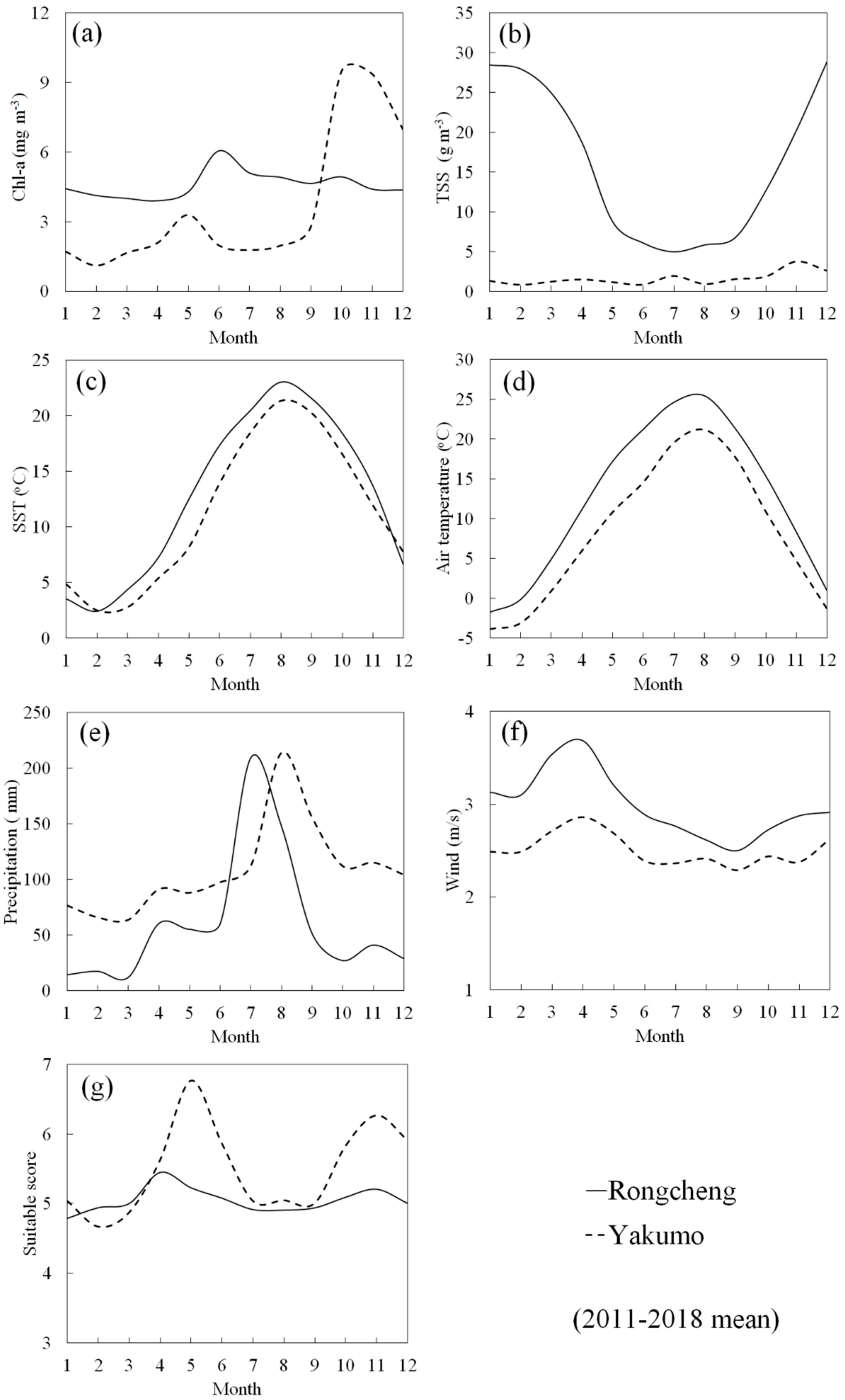
3.6. Seasonal Variability in Suitability Scores and Environmental, Meteorological, and Climate Factors

Using the newly developed SASSM, we generated the mean values of monthly suitability scores, environmental factors (Chl-a, TSS, and SST) and meteorological factors (temperature, precipitation, and wind) for each zone in Shandong and Funka Bay between 2011 and 2018. Among all zones, we the sites with the highest suitability were selected to represent each region (Yakumo for Funka Bay and Rongcheng for Shandong coasts, Figure 11). The peak of Chl-a concentration during spring (April-June) in Rongcheng was higher than those in Yakumo, however, in Yakumo region, the Chl-a bloom in autumn (October-November) was significantly higher than that in Rongcheng (Figure 11a). The seasonal variability of TSS in Rongcheng was highest in winter (December-March) and lowest in summer (July-September). However, the TSS concentration in Yakumo showed minimal fluctuations (Figure 11b). It is apparent that Rongcheng coastal waters are Case 2 waters, in which TSS may reach 35 g m−3. However, the Yakumo region is clearly Case 1 water, with maximum TSS below 3 g m−3. The average values of SST (Figure 11c) and air temperature (Figure 11d) were very similar in the two locations, which exhibited a minimum in January and a maximum in August. The SST and air temperature in Rongcheng were higher than those in Yakumo. The highest average values of precipitation in Rongcheng and Yakumo were in August and July, respectively (Figure 11e). The average wind speed in Rongcheng was obviously stronger than that in Yakumo, and was highest from winter to spring (December-April) and lowest in summer (August-September) (Figure 11f). The average suitability scores in Yakumo were higher than that in Rongcheng, and both locations had two peaks, one in spring (April-June) and one in autumn (October-November) (Figure 11g).
In order to highlight the impacts of climate variability in these two regions, monthly anomalies of environmental (Chl-a, TSS and SST) and meteorological factors (temperature, precipitation and wind) in both regions were examined for the period 2011–2018 (Figure 12). Winter East Asian monsoon (EAM) and ENSO (El Niño-Southern Oscillation) events have been identified as major drivers controlling winter climate over the North Pacific [38]. The monthly time series of the MOI anomaly and ONI indices during 2011–2018 (Figure 12h) showed that in the winter of 2011, the MOI was positive, which means that strong northerly winds prevailed over Northeast Asia from December to February [39]. Based on the monthly time series of ONI during 2011–2018 (Figure 12h), a very strong El Niño (ONI > 2) occurred during the winter of 2015–2016.
Combined with climate events index (MOI and ONI) variations, we noted that during strong El Niño event in 2015–2016, the Chl-a concentration anomaly at Yakumo in October was greater than the previous years (Figure 12a). The TSS anomaly in Rongcheng was positive in December 2016 and predominantly negative in winter 2018, however showed little change in Yakumo (Figure 12b). Likewise, SST and air temperature anomalies in winter of 2016 (December-March) at Yakumo were higher and lower in spring and summer of 2017 relative to other years (Figure 12c). However, during the normal years (2013 and 2014), the precipitation anomaly in summer (July-September) at Yakumo was higher than the El Niño and La Niña years (Figure 12e). The wind speed anomaly in January 2011 was the highest of all years (Figure 12f), however, showed a decreasing trend from 2011 to 2018. The air temperature anomaly in January 2011 at Rongcheng was also at its lowest (Figure 12d). It appears that the anomalies in monthly suitable score were strongly influenced by SST and air temperature (Figure 12g), as oceanic variability and atmospheric circulation are tightly coupled [40].

3.7. Correlations Among Climate Events, Environmental Factors, and Meteorological Factors

Variations in the climate and oceanic environment during winter (December–February) strongly influence scallop aquaculture in the spring. Figure 13 illustrates the relationships among these factors in Shandong during the winter season. Several significant correlations emerged from this analysis. MOI was strongly correlated with Chl-a, TSS and temperature. The ONI also showed strong negative correlation with wind (r= −0.69). Stronger winds may accelerate convective and eddy mixing [41,42], which in turn, could enhance TSS concentration as observed in satellite data. SST exhibited strong correlations with Chl-a (r = 0.63) and air temperature (r = 0.65).
Significant correlations among these factors in Funka Bay were also observed in winter between 2011 and 2018 (Figure 14). SST coupled with air temperature was strongly correlated with TSS and Chl-a, with precipitation strongly correlated with wind, Chl-a, TSS and SST. ONI was also correlated with temperature.

4. Discussion

The study identified assimilation of satellite data into GIS could provide useful information to identify spatial levels of suitability for scallop aquaculture. These technologies paid attention by much researchers to be used in planning and decision-making aquaculture activities [9,10,11,12,13,14]. SST, Chl-a and TSS could be extracted from ocean color satellite are often used as typical indicator for aquaculture research [4,5,6]. However, various type of satellite data limited not only on spatial and temporal resolutions, but also sources of accuracy. This study compared shipboard data with GOCI and MODIS illustrates that the latter had better Chl-a concentration accuracy than the former. From the comparisons between GOCI, GOCI filtered and MODIS monthly composites in existing aquaculture sites, correlations of Chl-a and TSS from GOCI and MODIS were relatively weak even after applying the filter operation. This may be due to the differences in algorithms used for calculating the science products [43]. In addition, there are sensor-specific differences. For one, MODIS is a polar-orbiting satellite sensor that collects data at about 1-km resolution once per day, whereas GOCI is a geostationary sensor that provides images every hour from 00:00 GMT to 07:00 GMT with 500-m resolution [16]. The high frequency of GOCI observations coupled with future improvement on the algorithms could possible prove hourly information for monitoring biological and physical processes in the northeast Asian coastal regions.
Through examining the correlations among climate events index, and environmental and climatic factors, we detected differences between Shandong coastal and Funka Bay. Our results indicate that MOI, ONI, wind, and SST play important roles in regulating the winter climate and marine environment in Shandong coastal region. Shandong peninsula not only affected by monsoon-influenced humid continental climate, but also oceanographically climate variations. The winter East Asia Monsoon driving strong northerly winds at the surface and along the China coasts, and shelf shallow-sea convective mixing and eddy mixing, which provide sufficient water exchange to supply nutrients for scallops [41,42,43,44]. SST in the northwestern Pacific shown high frequency variations associated with ENSO events [40]. in addition, strong wind could destroy the aquaculture facilities in the sea surface. Therefore, developing an integrated coastal aquaculture information system using satellite, buoy and numerical modeling data can be useful to monitor realistic wind and SST variations in Shandong coastal waters, which could provide early warning information for scallop aquaculture management. Previous studies have similarly reported significant correlations among ONI, Chl-a concentration, temperature and precipitation in Funka Bay [6]. Many studies have examined the influence of ENSO on temperature in East Asia [45,46] and highlighted the impact of heavy precipitation on salinity and phytoplankton dynamics in coastal regions [47]. Therefore, monitoring precipitation and temperature also important in Funka Bay.
During the past 8 years (2011–2018), we observed two extreme climate events, a strong positive MOI in winter 2011 and a strong El Niño event in 2015–2016. The Shandong Peninsula and Funka Bay are located in Northeast Asia, which is greatly impacted by EAM in winter. In addition, the dominant climate variability in the western North Pacific are high-frequency variations associated with ENSO events [37]. Comparison of climate indices (ENSO and MOI) and suitable areas in Weihai and Funka Bay across different years (2011–2016) during the growing season (May) highlighted differences. From these results, it is evident that the most suitable areas (scores 7 and 8) accounted for 15–20% of the Weihai coastal region (Table 4), and majority of the region was evaluated as medium suitability areas (scores 4, 5, and 6) for Japanese scallop aquaculture. This pattern is also apparent from the final SASSM maps for Shandong (Figure 9). Looking at the changes over time, the largest areas with score 7 (59.6%) in 2016 had likewise the highest total production, corresponded to a period with positive MOI and strong El Niño. Correlation analyses for environmental, meteorological factors and climate events confirmed that strong positive MOI and wind regulated the ocean and climate patterns in the Shandong coastal aquaculture region.
Using similar analysis for Funka Bay, most regions were found highly suitable for the Japanese scallop aquaculture, with scores of 6, 7, and 8 accounting for more than 95% of the total area every year (Table 5). The smallest suitable areas with scores of 7 (38.4%) and 8 (0.1%) were observed in 2017, when anomalously low SSTs in spring and summer were also observed. The SASSM maps (Figure 10) also reflected these patterns of decline in most suitable areas during this period, which could likely be a response to the lag in the climate impact of the strong El Niño event in 2016. The changes of most suitable areas were also evident from the lowest total production reported in 2017.On the other hand, highest spatial extent of most suitable areas (scores 8, 29.2%) was observed in 2012, corresponding to an anomalously high Chl-a concentration. Correlation analyses of environmental factors, meteorological factors, and climate events in Funka Bay further highlight the importance of ONI and SST on Japanese scallop aquaculture.
Comparison of the annual production of Japanese scallops between Shandong and Funka Bay presents difficulty in determining the relative quality of the two aquaculture areas. The spatial extents of both areas are different and scallop production is also influenced by factors such as the size of labor force, aquaculture management strategies, and the length of time in which aquaculture activities are in operation (three years in Funka Bay and one year in Shandong). However, in both regions, we have shown that climate events significantly affected the extent of suitable areas for Japanese scallop aquaculture, consistent with the results of the previous studies [4,5,9]. This work provides further support to the importance of environmental and climate monitoring towards sustainable aquaculture production and management in northeastern China and southern Hokkaido, Japan.

5. Conclusions

This study explored the feasibility of GOCI Chl-a and TSS data as complementary source for improving SASSM for the Japanese scallop aquaculture between two coastal regions (Shandong and Funka Bay). Our results suggested that GOCI products could prove useful for SASSM analyses and monitoring of coastal environment in high spatial and temporal resolution, with future improvement on the current algorithms used for deriving the ocean color products (Chl-a and TSS). The SASSM could also be improved by incorporating in situ and long term scallop growth observations to fit and verify the models. Our analyses revealed the impacts of climate variability to the availability of suitable sites in the two regions. In northeastern China, winter EAM was shown to affect the environment and climate dynamics in coastal aquaculture sites. Positive winter EAM, defined by low temperature and strong wind, is associated with Chl-a concentration enhancement in spring that could boost the scallop growth in Shandong coasts. In Funka Bay, ENSO events were also influential in regulating marine environmental dynamics., where El Niño events associated with precipitation, SST and Chl-a could significantly affect the availability of suitable areas. Undoubtedly, climatic events exert significant impacts on the extent of suitable areas for Japanese scallops across these regions and thus, climate dynamics should be considered in the management of coastal scallop aquaculture.

Author Contributions

S.-I.S. and Y.T. provided advises; K.-I.M. performed the experiments; I.D.A. checked the English text; Y.L. analyzed the data and wrote the paper. All authors have read and agreed to the published version of the manuscript.

Funding

This research was funded by the National Natural Science Foundation of China (No. 41976210), the Shandong Key R&D Program (No.2019GHY112014) and the Fundamental Research Funds for the Central Universities (No.201762015).

Acknowledgments

We thank two anonymous reviewers for their constructive comments.

Conflicts of Interest

The authors declare no conflict of interest.

References

  1. Jentsch, A.; Kreyling, J.; Beierkuhnlein, C. A new generation of climate-change experiments: Events, not trends. Front. Ecol. Environ. 2007, 5, 365–374. [Google Scholar] [CrossRef]
  2. Bai, X.Z.; Wang, J.; Liu, Q.Z.; Wang, D.X.; Liu, Y. Severe Ice Conditions in the Bohai Sea, China, and Mild Ice Conditions in the Great Lakes during the 2009/10 Winter: Links to El Niño and a Strong Negative Arctic Oscillation. J. Appl. Meteor. Climatol. 2011, 50, 1922–1935. [Google Scholar] [CrossRef]
  3. Strong El Niño, NOAA. Available online: https://www.noaa.gov/media-release/strong-el-ni-o-sets-stage-for-2015-2016-winter-weather (accessed on 9 January 2020).
  4. Hegerl, G.C.; Hanlon, H.; Beierkuhnlein, C. Climate science: Elusive extremes. Nat. Geosci. 2011, 4, 142–143. [Google Scholar] [CrossRef]
  5. Liu, Y.; Saitoh, S.-I.; Radiarta, I.N.; Isada, T.; Hirawake, T.; Mizuta, H.; Yasui, H. Improvement of an aquaculture site-selection model for Japanese kelp (Saccharina japonica) in southern Hokkaido, Japan: An application for the impacts of climate events. ICES J. Mar. Sci. 2013, 70, 1460–1470. [Google Scholar] [CrossRef] [Green Version]
  6. Liu, Y.; Saitoh, S.-I.; Igarashi, H.; Hirawake, T. The regional impacts of climate change on coastal environments and the aquaculture of Japanese scallops in northeast Asia: Case studies from Dalian, China and Funka Bay, Japan. Int. J. Remote Sens. 2014, 35, 4422–4440. [Google Scholar] [CrossRef]
  7. Bailey, H.; Secor, D. Coastal evacuations by fish during extreme weather events. Sci. Rep. 2016, 6, 30280. [Google Scholar] [CrossRef] [Green Version]
  8. FAO. The State of World Fisheries and Aquaculture 2018; Food and Agriculture Organization of the United Nations: Rome, Italy, 2018; p. 220. [Google Scholar]
  9. Li, Q.; Xu, K.F.; Yu, R.H. Genetic variation in Chinese hatchery population of the Japanese scallop (Mizuhopecten yessoensis) inferred from microsatellite data. Aquaculture 2007, 269, 211–219. [Google Scholar] [CrossRef]
  10. Liu, Y.; Saitoh, S.-I.; Radiarta, I.N.; Hirawake, T. Spatiotemporal variations in suitable areas for Japanese scallop aquaculture in Dalian, China from 2003 to 2012. Aquaculture 2014, 422–423, 172–183. [Google Scholar] [CrossRef] [Green Version]
  11. Kapetsky, J.M.; Anguilar–Manjarrez, J. Geographic Information Systems, Remote Sensing and Mapping for the Development and Management of Marine Aquaculture; FAO Fisheries Technical Paper No. 458; FAO: Rome, Italy, 2007; p. 125. [Google Scholar]
  12. Silva, C.; Ferreira, J.G.; Bricker, S.B.; Delvalls, T.A.; Martín-Díaz, M.L.; Yáñez, E. Site Selection for Shellfish Aquaculture by Means of GIS and Farm-Scale Models, with An Emphasis on Data-Poor Environments. Aquaculture 2011, 318, 444–457. [Google Scholar] [CrossRef]
  13. Radiarta, I.N.; Saitoh, S.-I.; Miyazono, A. GIS-Based Multi-Criteria Evaluation Models for Identifying Suitable Sites for Japanese Scallop (Mizuhopecten yessoensis) Aquaculture in Funka Bay, Southwestern Hokkaido, Japan. Aquaculture 2008, 284, 127–135. [Google Scholar] [CrossRef]
  14. Radiarta, I.N.; Saitoh, S.-I. Biophysical models for Japanese scallop, Mizuhopecten yessoensis, aquaculture site selection in Funka Bay, Hokkaido, Japan, using remotely sensed data and geographic information system. Aquac. Inter. 2009, 17, 403–419. [Google Scholar] [CrossRef]
  15. Saitoh, S.-I.; Mugo, R.; Radiarta, I.N.; Asaga, S.; Takahashi, F.; Hirawake, T.; Ishikawa, Y. Some operational uses of satellite remote sensing and marine GIS for sustainable fisheries and aquaculture. ICES J. Mar. Sci. 2011, 68, 687–695. [Google Scholar] [CrossRef] [Green Version]
  16. Ryu, J.H.; Han, H.J.; Cho, S.; Park, Y.J.; Ahn, Y.H. Overview of Geostationary Ocean Color Imager (GOCI) and GOCI data processing system (GDPS). Ocean Sci. J. 2012, 47, 223–233. [Google Scholar] [CrossRef]
  17. The Ministry of Agriculture of China. China Fishery Statistical Yearbook 2014; China Agriculture Press: Beijing, China, 2014. (In Chinese)
  18. Ohtani, K. Studies on the Change of the Hydrographic Conditions in the Funka Bay. Characteristics of the Water Occupying the Funka Bay. Bull. Fac. Fish. Hokkaido Univ. 1971, 22, 58–66. [Google Scholar]
  19. Marinenet Hokkaido. 2015. Search and Aggregate Statistics of the Fishery Catch from 1991 to 2016. Available online: https://www.hro.or.jp/list/fisheries/marine/index.html (accessed on 20 December 2019).
  20. NOAA Ocean Color. Available online: http://oceancolor.gsfc.nasa.gov (accessed on 9 January 2020).
  21. Ahn, Y.H.; Moon, J.E.; Gallegos, S. Development of suspended particulate matter algorithms for ocean color remote sensing. Korean J. Remote Sens. 2001, 17, 285–295. [Google Scholar]
  22. Korea Ocean Satellite Center (KOSC). Available online: http://kosc.kiost.ac.kr/eng/p30/kosc_p33.html (accessed on 9 January 2020).
  23. Siswanto, E.; Tang, J.; Yamaguchi, H.; Ahn, Y.H.; Ishizaka, J.; Yoo, S.; Kim, S.W.; Kiyomoto, Y.; Yamada, K.; Chiang, C.; et al. Empirical ocean-color algorithms to retrieve chlorophylla, total suspended matter, and colored dissolved organic matter absorption coefficient in the Yellow and East China Seas. J. Oceanogr. 2011, 67, 627–650. [Google Scholar] [CrossRef]
  24. O’Reilly, J.E.; Maritorena, S.; Siegel, D.A.; O’Brien, M.C.; Toole, D.; Mitchell, B.G.; Kahru, M.; Chavez, F.P.; Strutton, P.; Cota, G.F.; et al. Ocean color chlorophyll algorithms for SeaWiFS, OC2, and OC4: Version 4. In SeaWiFS Postlaunch Calibration and Validation Analyses; NASA Goddard Space Flight Center: Greenbelt, MD, USA, 2000; pp. 9–27. Available online: https://www.researchgate.net/publication/285869893_Ocean_chlorophyll_a_algorithms_for_Sea_WiFS_OC2_and_OC4_Version_4 (accessed on 20 December 2019).
  25. Yang, Q.; Du, L.B.; Liu, X.Y.; Hu, L.B.; Chen, S.G.; Liu, Y.; Wang, Z.Y.; Wang, Z.J.; Zhou, Y. Evaluation of ocean color products from Korean Geostationary Ocean Color Imager (GOCI) in Jiaozhou Bay and Qingdao coastal area. In Proceedings of the SPIE Asia-Pacific Remote Sensing, Beijing, China, 18 December 2014. [Google Scholar] [CrossRef]
  26. ALOS User Interface Gateway (AUIG). Available online: https://auig2.jaxa.jp/ips/home (accessed on 9 January 2020).
  27. United States Geological Survey Earth Resources Observation Satellites (USGS EROS). Available online: https://earthexplorer.usgs.gov/ (accessed on 9 January 2020).
  28. National Meteorological Information Center of China Meteorological Administration. Available online: http://data.cma.cn/site/index.html (accessed on 9 January 2020).
  29. Japan Meteorological Agency (JMA). Available online: http://www.jma.go.jp/jma/indexe.html (accessed on 9 January 2020).
  30. Hanawa, K.; Watanabe, T.; Iwasaka, N.; Suga, T.; Toba, Y. Surface Thermal Conditions in the Western North Pacific during the ENSO Events. J. Meteor. Soc. Japan. 1988, 66, 445–456. [Google Scholar] [CrossRef] [Green Version]
  31. NCEP Reanalysis Database. Available online: http://www.esrl.noaa.gov/psd/ (accessed on 9 January 2020).
  32. National Weather Service, Center for Climate Prediction, NOAA. Available online: https://origin.cpc.ncep.noaa.gov/products/analysis_monitoring/ensostuff/ONI_change.shtml (accessed on 9 January 2020).
  33. Stachelski, C.; Czyzyk, S. El Niño and La Niña episodes and their impact on the weather in the Las Vegas Valley. Available online: https://www.weather.gov/media/wrh/online_publications/talite/talite0903.pdf (accessed on 9 January 2020).
  34. Liu, Y.; Saitoh, S.-I.; Nakada, S.; Zhang, X.; Hirawake, T. Impact of Oceanographic Environmental Shifts and Atmospheric Events on the Sustainable Development of Coastal Aquaculture: A case Study of Kelp and Scallops in Southern Hokkaido, Japan. Sustainability 2015, 7, 1263–1279. [Google Scholar] [CrossRef] [Green Version]
  35. Saaty, T.L. A Scaling Method for Priorities in Hierarchical Structures. J. Math. Psychol. 1977, 15, 234–281. [Google Scholar] [CrossRef]
  36. Malczewski, J. On the Use of Weighted Linear Combination Method in GIS: Common and Best Practice Approaches. Trans. GIS 2000, 4, 5–22. [Google Scholar] [CrossRef]
  37. Ito, H. Patinopecten (Mizuhopecten) yessoensis. In Scallops: Biology, Ecology and Aquaculture; Shumway, S.E., Parsons, G.J., Eds.; Elsevier: Amsterdam, The Netherlands, 1991; pp. 1024–1055. [Google Scholar]
  38. Zhang, R.H.; Sumi, A.; Kimoto, M. Impact of El Niño on the East Asian monsoon: a diagnostic study of the 86/87 and 91/92 events. J. Meteorol. Soc. Jpn. 1996, 74, 49–62. [Google Scholar] [CrossRef] [Green Version]
  39. Naimie, C.E.; Blain, C.A.; Lynch, D.R. Seasonal Mean Circulation in the Yellow Sea–A Model-Generated Climatology. Cont. Shelf Res. 2001, 21, 667–695. [Google Scholar] [CrossRef]
  40. Mckinnell, S.M.; Dagg, M.J. Marine Ecosystems of the North Pacific Ocean, 2003–2008. PICES Special Publication 2010, 4, 393. Available online: http://imecocal.cicese.mx/publicaciones/divulgacion/PICES_pub4_Chp3_California.pdf (accessed on 9 January 2020).
  41. Ma, J.; Qiao, F.L.; Xia, C.S.; Kim, C.S. Effects of the Yellow SeaWarm Current on the Winter Temperature Distribution in a Numerical Model. J. Geophys. Res. 2006, 111, C11S04. [Google Scholar] [CrossRef] [Green Version]
  42. Huang, R.H.; Chen, J.L.; Huang, G. Characteristics and Variations of the East Asian Monsoon System and Its Impacts on Climate Disasters in China. Adv. Atmos. Sci. 2007, 24, 993–1023. [Google Scholar] [CrossRef]
  43. Lyu, H.; Zhang, J.; Zha, G.H.; Wang, Q.; Li, Y.M. Developing a two-step retrieval method for estimating total suspended solid concentration in Chinese turbid inland lakes using Geostationary Ocean Colour Imager (GOCI) imagery. Int. J. Remote Sens. 2015, 36, 1385–1405. [Google Scholar] [CrossRef]
  44. Liu, W.L.; Qian, L.; Zheng, X.S. Spatial-Temporal Variation of Chlorophyll-A Concentration in the Bohai Sea. In Proceedings of the International Conference on Life System Modeling and Simulation, LSMS 2010, and International Conference on Intelligent Computing for Sustainable Energy and Environment, ICSEE 2010, Wuxi, China, 17–20 September 2010. [Google Scholar]
  45. Seager, B.R.; Harnik, N.; Robinson, W.A.; Kushnir, Y.; Ting, M.; Huang, H.P.; Velez, J. Mechanisms of Enso-Forcing of Hemi Spherically Symmetric Precipitation Variability. Q. J. Roy. Meteor. Soc. 2005, 131, 1501–1527. [Google Scholar] [CrossRef] [Green Version]
  46. Son, H.Y.; Park, J.Y.; Kug, J.S. Winter Precipitation Variability over East Asia Associated with ENSO. Geophys. Res. Abstr. 2012, 14, 6874. [Google Scholar]
  47. Acker, J.G.; Hardding, L.W.; Leptoukh, G.; Zhu, T.; Shen, S.H. Remotely-Sensed Chl-A at the Chesapeake Bay Mouth Is Correlated with Annual Freshwater Flow to Chesapeake Bay. Geophys. Res. Lett. 2005, 32, L05601. [Google Scholar] [CrossRef]
Figure 1. Study area of scallop zones and sampling stations in Shandong (top left) and Funka Bay (bottom right), respectively. Scallop aquaculture sites in Funka Bay are further divided into eight zones represented by the colored polygons. The sampling sites for oceanographic surveys conducted within the Funka Bay between May 2011 and January 2012 are denoted by the solid dots.
Sustainability 12 00833 g001
Figure 2. Annual production of Japanese scallop for each zone in Funka Bay between 2011 and 2017.
Sustainability 12 00833 g002
Figure 3. Schematic flow of analyses conducted in this study, highlighting the different data platforms incorporated to improve the earlier version of the suitable aquaculture site-selection model (SASSM) for Japanese scallop.
Sustainability 12 00833 g003
Figure 4. Comparisons of shipboard Chl-a measurements with (a) GOCI–derived and (b) MODIS-derived Chl-a concentration over five cruises, and comparison between (c) GOCI- and MODIS-derived Chl-a measurements.
Sustainability 12 00833 g004
Figure 5. Monthly composited Chl-a and total suspended sediment (TSS) concentrations from (a,d) GOCI, (b,e) GOCI-filtered, and (c,f) MODIS for May 2011. Existing aquaculture sites are enclosed in red-colored polygons.
Sustainability 12 00833 g005
Figure 6. Comparisons of monthly Chl-a and TSS concentrations between (a,d) GOCI and GOCI-filtered, (b,e) GOCI and MODIS, and (c,f) GOCI-filtered and MODIS- derived measurements in Funka Bay, May 2011.
Sustainability 12 00833 g006
Figure 7. Suitable site maps for Japanese scallop aquaculture based on yearly mean data from May 2011 to April 2012 using (a) the previous model, (b) the SASSM with GOCI Chl-a concentration data, (c) the newly developed SASSM with GOCI Chl-a concentration data, and (d) the newly developed SASSM with GOCI Chl-a concentration and TSS data. The red box area is existing aquaculture region.
Sustainability 12 00833 g007
Figure 8. Monthly score comparisons between (a) new and previous SASSMs, (b) AMW of scallop with new SASSM, and (c) AMW of scallop with previous SASSM, between 2011 and 2013 at Yakumo station.
Sustainability 12 00833 g008
Figure 9. SASSM maps for Japanese scallop during the growing season (May) along the Shandong, 2011–2018.
Sustainability 12 00833 g009
Figure 10. SASSM maps for Japanese scallop during the growing season (May) along the coastal waters of Funka Bay, 2011–2018.
Sustainability 12 00833 g010
Figure 11. Seasonal changes in the average values of (a) Chl-a concentration, (b) TSS, (c) SST, (d) air temperature, (e) precipitation, (f) wind speed, and (g) suitable score in Rongcheng, Shandong and Yakumo, Funka bay from 2011 to 2018. TSS: total suspended sediment, SST: sea surface temperature.
Sustainability 12 00833 g011
Figure 12. Time series of monthly anomaly (a) Chl-a concentration, (b) TSS, (c) SST, (d) air temperature, (e) precipitation, (f) wind speed, (g) suitability score, and (h) climate event indices (ONI and MOI) in Shandong and Funka Bay from 2011 to 2018. SST: sea surface temperature; TSS: total suspended sediment; ONI: Oceanic Niño index; MOI: monsoon index.
Sustainability 12 00833 g012
Figure 13. Correlations among climate event factors, environmental factors and meteorological factors in Shandong in winter (December–February) 2011–2018. Values in the cells above the diagonal are Pearson’s correlation coefficients, scales the correlation font by the size of the absolute correlation. *Correlation is significant at the 0.05 level. Temp: air temperature (°C); Preci: precipitation (mm/year); Wind: wind speed (m/s); Chl: Chl-a concentration (mg/m3); TSS: total suspended sediment (g/l3) SST: sea surface temperature (°C); ONI: Oceanic Niño index; MOI: monsoon index.
Sustainability 12 00833 g013
Figure 14. Correlations among climate event factors, environmental factors and meteorological factors in Funka Bay in winter (December–February) 2011–2018. Values in the cells above the diagonal are Pearson’s correlation coefficients, scales the correlation font by the size of the absolute correlation. *Correlation is significant at the 0.05 level. Temp: air temperature (°C); Preci: precipitation (mm/year); Wind: wind speed (m/s); Chl: Chl-a concentration (mg/m3); TSS: total suspended sediment (g/l3) SST: sea surface temperature (°C); ONI: Oceanic Niño index; MOI: monsoon index.
Sustainability 12 00833 g014
Table 1. Summary information on oceanographic cruises in Funka Bay onboard the RV Ushio-Maru (May 2011–Jan 2012). The number of samples (n) for ship-board observations and satellite-derived measurements from MODIS and GOCI were also noted.
YearCruiseIn-SituGOCIMODIS
DatenDatenDaten
2011US22814–16 May2315 May2118 May14
2011US23227–28 Jul1331 Jul822 Jul6
2011US23727–29 Sep828 Sep8
2011US24217–19 Nov1018 Nov712 Nov10
2012US24610 Jan58 Jan57 Jan5
Table 2. Physical requirements and suitability scores for Japanese scallop SASSM adjusted for GOCI in southern Hokkaido, Japan.
Suitability Rating and Score
Parameter12345678
Sea Surface
temperature (°C)
<44–55–66–77–88–99–1010–11
17–3516–1715–1614–1513–1412–1311–12
Bathymetry (m)0–33–55–77–99–1111–1313–1515–60
Total suspended sediment (g m−3)4.1 <3.6–4.13.1–3.62.6–3.12.1–2.61.6–2.11.1–1.60–1.1
Chl-a (mg m−3)0–0.40.4–0.60.6–0.80.8–1.21.2–1.61.6–2.02.0–2.22.2 <
Table 3. Different suitability levels (expressed as percentage of total aquaculture area) for each combination of parameters and scoring systems for SASSMs in Funka Bay, developed using annual model averages from May 2011–April 2012.
ParameterScoring SystemSuitability Scores (%)
Chl-aSSTTSS345678
MODISMODISMODISPrevious0.00.40.812.768.617.5
GOCIMODISMODISPrevious0.00.10.62.935.760.7
GOCIMODISMODISNew developed0.10.52.923.958.314.3
GOCIMODISGOCINew developed0.01.13.717.558.719.1
Table 4. Differences in site suitability (expressed as a percentage of the total potential area) between EAM-influenced and normal growing seasons in Weihai, China. MOI: monsoon index, ENSO: El Niño/La Niña Southern Oscillation. The scallop production data in both regions were only reported until 2016.
YearSuitability Scores (%)MOI
in winter
ENSO Event
in winter
Total Annual Production
(104 tonnes) [17]
34567
May 20116.816.935.520.020.8Strong positiveModerate La Niña16.8
May 20124.723.821.929.020.5PositiveWeak La Niña16.0
May 20136.211.335.431.016.0NegativeNormal16.1
May 201412.912.135.920.218.9NegativeNormal15.5
May 20156.612.339.721.919.5PositiveWeak El Niño17.4
May 20160.43.524.811.759.6PositiveStrong El Niño18.1
May 20175.115.732.443.53.3NegativeWeak La Niña
May 20187.012.536.229.614.6Positive Weak La Niña
Table 5. Differences in site suitability (expressed as a percentage of the total potential area) between ENSO-influenced and normal growing seasons in Funka Bay, Japan. MOI: monsoon index, ENSO: El Niño/La Niña Southern Oscillation.
YearSuitability Scores (%)MOI
in winter
ENSO Event
in winter
Total Annual Production
(104 tonnes) [19]
5678
May 20110.717.470.011.8Strong positiveModerate La Niña5.8
May 20120.14.466.229.2PositiveWeak La Niña7.5
May 20130.39.572.517.7NegativeNormal8.2
May 20140.519.672.17.8NegativeNormal8.1
May 20150.13.774.621.6PositiveWeak El Niño10.4
May 20160.06.881.311.9PositiveStrong El Niño5.6
May 201712.049.438.40.1NegativeWeak La Niña2.6
May 20181.120.875.13.0PositiveWeak La Niña

