Method of Predicting Ore Dilution Based on a Neural Network and Its Application

Abstract
:1. Introduction
2. Materials and Methodologies
2.1. Parameter Selection and Data Acquisition
2.2. Neural Network Model
2.2.1. Model Structure
2.2.2. Building the Model
2.2.3. Model Training and Testing
2.2.4. Calculation of Unplanned Ore Dilution
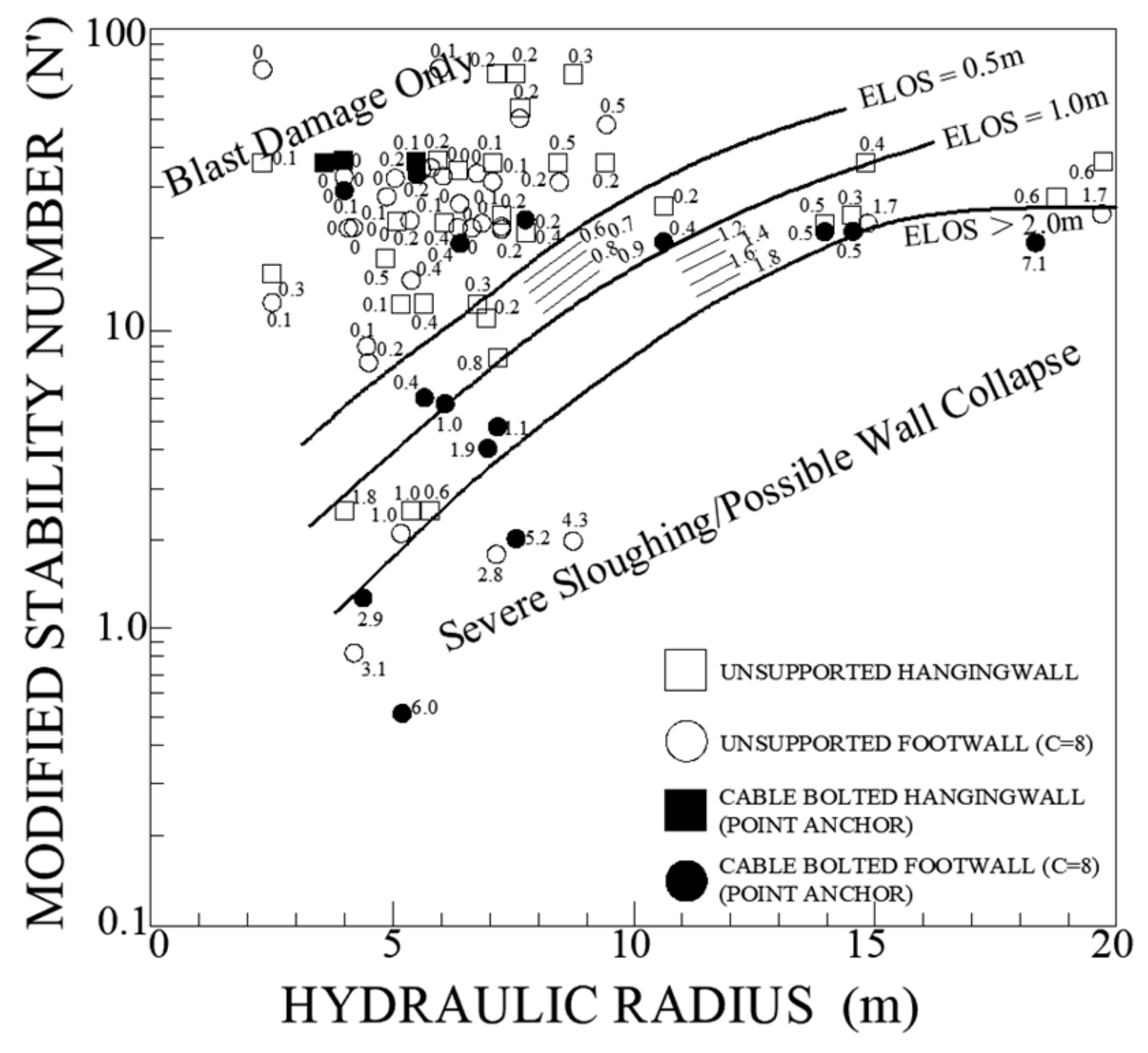
2.3. Empirical Graph Method
2.4. Numerical Simulation Method
3. Results
3.1. Engineering Application
3.1.1. Geological Setting and Engineering Background
3.1.2. Test Stope
3.1.3. Model Application
3.2. Comparison and Analysis
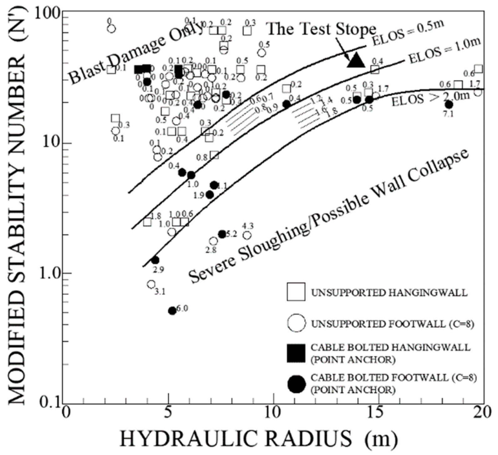
3.2.1. Results of Empirical Graph Method
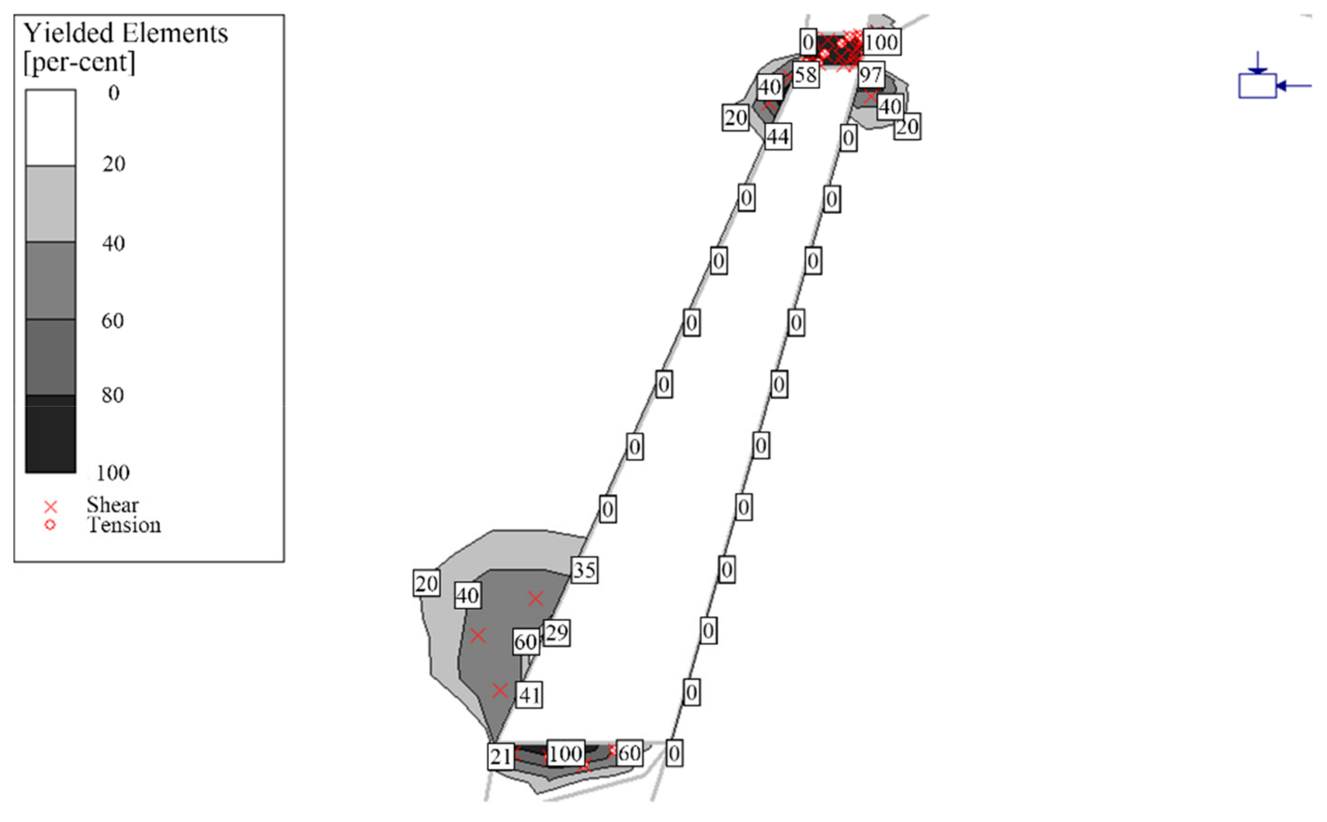
3.2.2. Results of Numerical Simulation
4. Discussion
5. Conclusions
Author Contributions
Funding
Conflicts of Interest
Appendix A

| Sample Number | Modified Stability Number | Hydraulic Radius (m) | Average Borehole Deviation (m) | Powder Factor (kg/t) | ELOS (m) |
|---|---|---|---|---|---|
| 1 | 73.10 | 10.46 | 0.50 | 0.50 | 0.10 |
| 2 | 29.36 | 12.95 | 0.60 | 0.50 | 1.10 |
| 3 | 0.17 | 1.82 | 0.20 | 0.39 | 2.70 |
| 4 | 11.25 | 7.38 | 0.40 | 0.58 | 1.20 |
| 5 | 35.07 | 8.46 | 0.40 | 0.58 | 0.90 |
| 6 | 9.28 | 6.00 | 0.30 | 0.50 | 0.60 |
| 7 | 18.19 | 13.68 | 0.60 | 0.50 | 1.90 |
| 8 | 10.39 | 6.89 | 0.30 | 0.45 | 0.70 |
| 9 | 6.93 | 6.89 | 0.30 | 0.45 | 1.10 |
| 10 | 35.28 | 4.05 | 0.40 | 0.58 | 0.10 |
| 11 | 9.18 | 4.05 | 0.40 | 0.58 | 0.40 |
| 12 | 35.28 | 6.12 | 0.40 | 0.58 | 0.10 |
| 13 | 9.18 | 6.12 | 0.40 | 0.58 | 0.70 |
| 14 | 14.03 | 3.78 | 0.40 | 0.39 | 0.30 |
| 15 | 3.81 | 3.78 | 0.40 | 0.39 | 0.80 |
| 16 | 14.03 | 5.51 | 0.40 | 0.39 | 0.40 |
| 17 | 3.81 | 5.51 | 0.40 | 0.39 | 1.30 |
| 18 | 14.03 | 6.51 | 0.40 | 0.39 | 0.40 |
| 19 | 3.81 | 6.51 | 0.40 | 0.39 | 1.80 |
| 20 | 1.81 | 1.78 | 0.20 | 0.45 | 1.00 |
| 21 | 8.10 | 7.00 | 0.50 | 0.56 | 0.80 |
| 22 | 11.00 | 7.40 | 0.60 | 0.41 | 1.30 |
| 23 | 7.00 | 8.80 | 0.60 | 0.64 | 2.30 |
| 24 | 11.00 | 7.30 | 0.70 | 0.45 | 2.10 |
| 25 | 7.10 | 9.30 | 1.00 | 0.95 | 1.30 |
| 26 | 8.80 | 6.90 | 0.10 | 0.59 | 0.10 |
| 27 | 7.80 | 7.60 | 0.60 | 0.41 | 1.10 |
| 28 | 8.80 | 6.70 | 0.70 | 0.86 | 2.10 |
| 29 | 7.30 | 7.20 | 0.30 | 0.36 | 1.20 |
| 30 | 7.80 | 6.90 | 0.70 | 0.45 | 1.90 |
| 31 | 10.80 | 5.00 | 0.50 | 0.41 | 0.60 |
| 32 | 8.00 | 7.20 | 0.4 | 0.40 | 1.20 |
| 33 | 12.20 | 6.60 | 0.20 | 0.40 | 0.20 |
| 34 | 11.40 | 6.70 | 0.30 | 0.41 | 0.50 |
| 35 | 6.70 | 7.30 | 0.20 | 0.59 | 1.10 |
| 36 | 12.00 | 6.20 | 0.20 | 0.60 | 0.40 |
| 37 | 9.90 | 9.10 | 0.4 | 0.88 | 1.40 |
| 38 | 14.10 | 5.40 | 0.40 | 0.37 | 0.20 |
| 39 | 9.20 | 6.00 | 0.60 | 0.45 | 0.50 |
| 40 | 12.20 | 6.60 | 0 | 0.43 | 0.30 |
| 41 | 11.20 | 5.50 | 0 | 0.59 | 0.40 |
| 42 | 11.10 | 5.20 | 0.50 | 0.52 | 0.40 |
| 43 | 6.00 | 5.50 | 0.75 | 1.05 | 3.30 |
| 44 | 11.10 | 6.20 | 0 | 0.40 | 0.40 |
| 45 | 11.60 | 6.50 | 0.50 | 0.50 | 0.60 |
| 46 | 6.30 | 8.00 | 1.00 | 0.41 | 4.40 |
| 47 | 9.80 | 7.00 | 1.20 | 0.28 | 4.00 |
| 48 | 12.00 | 6.30 | 0.40 | 0.32 | 0.70 |
| 49 | 13.50 | 6.90 | 0.40 | 0.54 | 0.60 |
| 50 | 9.80 | 7.50 | 0.50 | 0.32 | 0.80 |
| 51 | 11.00 | 6.00 | 0.40 | 0.67 | 0.40 |
| 52 | 10.10 | 8.10 | 0.90 | 0.51 | 1.10 |
| 53 | 9.50 | 6.20 | 0.80 | 0.47 | 0.70 |
| 54 | 10.30 | 6.30 | 0.70 | 0.47 | 0.60 |
| 55 | 8.20 | 6.00 | 0.90 | 0.29 | 1.10 |
| 56 | 7.70 | 5.60 | 0.90 | 0.47 | 1.50 |
| 57 | 8.20 | 5.70 | 0.90 | 0.36 | 2.40 |
| 58 | 9.10 | 5.70 | 0.30 | 0.31 | 0.80 |
| 59 | 10.40 | 6.90 | 0.60 | 0.57 | 0.80 |
| 60 | 10.60 | 5.70 | 0.70 | 0.33 | 0.40 |
| 61 | 4.50 | 7.20 | 1.00 | 0.30 | 1.90 |
| 62 | 7.90 | 7.20 | 0 | 0.30 | 0.90 |
| 63 | 3.80 | 7.00 | 0.50 | 0.25 | 1.90 |
| 64 | 5.40 | 6.10 | 0.90 | 0.25 | 1.20 |
| 65 | 5.60 | 5.70 | 0 | 0.45 | 0.40 |
| 66 | 12.00 | 5.70 | 0 | 0.45 | 0.30 |
| 67 | 1.70 | 7.20 | 0 | 0.60 | 2.80 |
| 68 | 7.20 | 7.20 | 0 | 0.60 | 0.20 |
| 69 | 1.90 | 8.80 | 0 | 0.40 | 4.30 |
| 70 | 72.00 | 8.80 | 0 | 0.40 | 0.20 |
| 71 | 1.90 | 7.60 | 0 | 0.55 | 5.20 |
| 72 | 72.00 | 7.60 | 0 | 0.55 | 0.10 |
| 73 | 34.00 | 10.20 | 0 | 0.40 | 0 |
| 74 | 18.20 | 4.50 | 0 | 0.39 | 0.20 |
| 75 | 21.60 | 4.50 | 0 | 0.39 | 0.10 |
| 76 | 21.60 | 7.30 | 0.60 | 0.31 | 0.30 |
| 77 | 21.60 | 7.30 | 0.60 | 0.31 | 0.30 |
| 78 | 21.60 | 6.70 | 1.10 | 0.32 | 0.50 |
| 79 | 21.60 | 6.40 | 0.90 | 0.32 | 0.40 |
| 80 | 1.20 | 4.40 | 0 | 0.70 | 2.90 |
| 81 | 22.50 | 15.00 | 0.25 | 0.65 | 1.90 |
| 82 | 36.00 | 15.00 | 0.25 | 0.65 | 1.00 |
| 83 | 22.50 | 20.00 | 0.25 | 0.65 | 4.10 |
| 84 | 36.00 | 20.00 | 0.25 | 0.65 | 1.70 |
| 85 | 34.00 | 5.80 | 0.60 | 0.90 | 0.10 |
| 86 | 2.40 | 5.80 | 0.30 | 0.90 | 2.00 |
| 87 | 12.00 | 2.50 | 0.40 | 0.50 | 0.10 |
| 88 | 15.00 | 2.50 | 0.40 | 0.50 | 0.30 |
| 89 | 23.00 | 5.40 | 0.50 | 1.20 | 0.20 |
| 90 | 2.40 | 5.40 | 0.10 | 1.20 | 1.80 |
| 91 | 22.00 | 4.10 | 0.10 | 1.10 | 0.20 |
| 92 | 23.00 | 4.10 | 0.10 | 1.10 | 0.10 |
| 93 | 29.00 | 4.00 | 0.50 | 0.58 | 0.10 |
| 94 | 36.00 | 4.00 | 0.95 | 0.58 | 0.10 |
| 95 | 32.00 | 4.00 | 0.30 | 0.90 | 0.10 |
| 96 | 2.40 | 4.00 | 0.15 | 0.90 | 1.10 |
| 97 | 22.00 | 4.20 | 0.10 | 1.20 | 0.10 |
| 98 | 23.00 | 4.20 | 0.10 | 1.20 | 0 |
| 99 | 32.00 | 5.10 | 0.30 | 0.63 | 0.30 |
| 100 | 23.00 | 5.10 | 0.40 | 0.63 | 0.20 |
| 101 | 14.50 | 5.40 | 0.50 | 1.00 | 0.40 |
| 102 | 2.40 | 5.40 | 0.15 | 1.00 | 1.80 |
| 103 | 35.00 | 5.60 | 0 | 1.14 | 0.10 |
| 104 | 23.00 | 5.60 | 0 | 1.14 | 0.30 |
| 105 | 26.00 | 6.40 | 0.80 | 0.65 | 0.20 |
| 106 | 34.00 | 6.40 | 0.50 | 0.65 | 0.10 |
| 107 | 28.00 | 4.90 | 1.00 | 0.47 | 0.40 |
| 108 | 17.00 | 4.90 | 0.45 | 0.47 | 0.40 |
| 109 | 22.40 | 6.90 | 0.40 | 0.84 | 0.20 |
| 110 | 23.00 | 6.90 | 0.30 | 0.84 | 0.20 |
| 111 | 10.50 | 5.60 | 0.30 | 1.19 | 0.40 |
| 112 | 23.00 | 5.60 | 0 | 1.19 | 0.20 |
| 113 | 2.00 | 5.20 | 0.50 | 0.64 | 1.80 |
| 114 | 12.00 | 5.20 | 0.50 | 0.64 | 0.50 |
| 115 | 31.00 | 7.10 | 0.15 | 0.84 | 0.20 |
| 116 | 36.00 | 7.10 | 0.15 | 0.84 | 0.10 |
| 117 | 33.00 | 5.50 | 0.15 | 1.05 | 0.10 |
| 118 | 7.10 | 8.10 | 0 | 0.35 | 1.60 |
| 119 | 60.00 | 7.90 | 0.50 | 0.45 | 0.20 |
| 120 | 7.20 | 7.30 | 0 | 1.22 | 1.20 |
Appendix B
| Sample Number | Measured Value (m) | Predicted Value (m) | Relative Error (%) | Sample Number | Measured Value (m) | Predicted Value (m) | Relative Error (%) |
|---|---|---|---|---|---|---|---|
| Ⅰ-1 | |||||||
| 1 | 0.40 | 0.4016 | 0.4 | 13 | 1.90 | 1.8510 | 2.6 |
| 2 | 0.10 | 0.1096 | 9.6 | 14 | 0.80 | 0.8726 | 9.1 |
| 3 | 0.20 | 0.2179 | 8.9 | 15 | 0.20 | 0.1932 | 3.4 |
| 4 | 0.70 | 0.7025 | 0.4 | 16 | 0.50 | 0.5363 | 7.3 |
| 5 | 0.70 | 0.7625 | 8.9 | 17 | 4.30 | 4.6840 | 8.9 |
| 6 | 0.30 | 0.3256 | 8.5 | 18 | 3.30 | 3.5360 | 7.2 |
| 7 | 0.10 | 0.0984 | 1.6 | 19 | 0.10 | 0.0896 | 10.4 |
| 8 | 0.40 | 0.4363 | 9.1 | 20 | 2.00 | 2.1350 | 6.8 |
| 9 | 0.30 | 0.3260 | 8.7 | 21 | 0.40 | 0.4254 | 6.4 |
| 10 | 0.50 | 0.5104 | 2.1 | 22 | 0.80 | 0.7242 | 9.5 |
| 11 | 0.60 | 0.5619 | 6.4 | 23 | 0.90 | 0.9262 | 2.9 |
| 12 | 0.90 | 0.8672 | 3.6 | 24 | 1.10 | 1.1210 | 1.9 |
| Ⅰ-2 | |||||||
| 1 | 2.70 | 2.8167 | 4.3 | 13 | 1.80 | 1.7164 | 4.6 |
| 2 | 0.00 | 0.0125 | - | 14 | 1.80 | 1.8591 | 3.3 |
| 3 | 1.10 | 1.1294 | 2.7 | 15 | 0.40 | 0.3916 | 2.1 |
| 4 | 0.10 | 0.1165 | 16.5 | 16 | 0.10 | 0.0898 | 10.2 |
| 5 | 0.20 | 0.2088 | 4.4 | 17 | 0.20 | 0.2211 | 10.6 |
| 6 | 0.40 | 0.4376 | 9.4 | 18 | 0.20 | 0.2017 | 0.8 |
| 7 | 0.70 | 0.6153 | 12.1 | 19 | 1.70 | 1.5946 | 6.2 |
| 8 | 1.00 | 1.0768 | 7.7 | 20 | 1.10 | 1.0579 | 3.8 |
| 9 | 1.30 | 1.3013 | 0.1 | 21 | 1.20 | 1.1350 | 5.4 |
| 10 | 0.20 | 0.1936 | 3.2 | 22 | 0.20 | 0.1960 | 2.0 |
| 11 | 0.20 | 0.1867 | 6.7 | 23 | 0.10 | 0.0863 | 13.7 |
| 12 | 0.20 | 0.1962 | 1.9 | 24 | 1.80 | 2.0341 | 13.0 |
| Ⅰ-3 | |||||||
| 1 | 0.40 | 0.4312 | 7.8 | 13 | 0.20 | 0.1843 | 7.9 |
| 2 | 0.10 | 0.1163 | 16.3 | 14 | 1.90 | 2.1185 | 11.5 |
| 3 | 0.10 | 0.0897 | 10.3 | 15 | 2.40 | 2.5134 | 4.7 |
| 4 | 0.40 | 0.3848 | 3.8 | 16 | 4.10 | 4.2107 | 2.7 |
| 5 | 0.40 | 0.4132 | 3.3 | 17 | 0.60 | 0.5861 | 2.3 |
| 6 | 0.40 | 0.4076 | 1.9 | 18 | 0.40 | 0.4166 | 4.2 |
| 7 | 0.30 | 0.3189 | 6.3 | 19 | 2.30 | 2.5427 | 10.6 |
| 8 | 1.60 | 1.6931 | 5.8 | 20 | 0.30 | 0.3166 | 5.5 |
| 9 | 0.40 | 0.3977 | 0.6 | 21 | 0.20 | 0.1843 | 7.9 |
| 10 | 1.20 | 1.2694 | 5.8 | 22 | 0.00 | 0.0000 | - |
| 11 | 0.30 | 0.2849 | 5.0 | 23 | 1.20 | 1.2309 | 2.6 |
| 12 | 1.90 | 2.1067 | 10.9 | 24 | 0.10 | 0.1129 | 12.9 |
| Ⅰ-4 | |||||||
| 1 | 1.30 | 1.3351 | 2.7 | 13 | 1.40 | 1.3527 | 3.4 |
| 2 | 1.20 | 1.1964 | 0.3 | 14 | 2.80 | 3.1640 | 13.0 |
| 3 | 2.90 | 3.1360 | 8.1 | 15 | 5.20 | 4.9937 | 4.0 |
| 4 | 2.10 | 2.2034 | 4.9 | 16 | 1.80 | 1.8324 | 1.8 |
| 5 | 1.10 | 1.0875 | 1.1 | 17 | 1.10 | 1.2165 | 10.6 |
| 6 | 1.50 | 1.6137 | 7.6 | 18 | 0.10 | 0.1183 | 18.3 |
| 7 | 0.60 | 0.5873 | 2.1 | 19 | 1.30 | 1.3065 | 0.5 |
| 8 | 4.00 | 3.8992 | 2.5 | 20 | 0.40 | 0.4324 | 8.1 |
| 9 | 0.80 | 0.8443 | 5.5 | 21 | 0.80 | 0.8735 | 9.2 |
| 10 | 0.40 | 0.4385 | 9.6 | 22 | 1.90 | 2.0415 | 7.4 |
| 11 | 0.40 | 0.3768 | 5.8 | 23 | 1.10 | 1.1216 | 2.0 |
| 12 | 0.10 | 0.0879 | 12.1 | 24 | 0.60 | 0.6370 | 6.2 |
| Ⅰ-5 | |||||||
| 1 | 0.30 | 0.2843 | 5.2 | 13 | 0.50 | 0.4735 | 5.3 |
| 2 | 1.90 | 1.8463 | 2.8 | 14 | 0.60 | 0.5783 | 3.6 |
| 3 | 0.20 | 0.2174 | 8.7 | 15 | 0.10 | 0.1008 | 0.8 |
| 4 | 0.30 | 0.3149 | 5.0 | 16 | 0.20 | 0.2101 | 5.1 |
| 5 | 0.10 | 0.0889 | 11.1 | 17 | 0.80 | 0.8345 | 4.3 |
| 6 | 0.40 | 0.3974 | 0.7 | 18 | 2.10 | 2.0762 | 1.1 |
| 7 | 0.20 | 0.1865 | 6.8 | 19 | 0.10 | 0.1015 | 1.5 |
| 8 | 0.30 | 0.3348 | 11.6 | 20 | 0.10 | 0.0991 | 0.9 |
| 9 | 0.10 | 0.1176 | 17.6 | 21 | 1.20 | 1.2016 | 0.1 |
| 10 | 1.10 | 1.2840 | 16.7 | 22 | 0.50 | 0.4870 | 2.6 |
| 11 | 4.40 | 4.0957 | 6.9 | 23 | 1.00 | 1.1047 | 10.5 |
| 12 | 0.70 | 0.6782 | 3.1 | 24 | 0.10 | 0.0985 | 1.5 |
| Ⅱ-1 | |||||||
| 1 | 1.90 | 1.8967 | 0.2 | 13 | 0.20 | 0.1980 | 1.0 |
| 2 | 0.40 | 0.3955 | 1.1 | 14 | 1.90 | 2.0766 | 9.3 |
| 3 | 0.10 | 0.1103 | 10.3 | 15 | 0.40 | 0.3754 | 6.2 |
| 4 | 0.40 | 0.4124 | 3.1 | 16 | 0.10 | 0.0955 | 4.5 |
| 5 | 0.20 | 0.2067 | 3.3 | 17 | 0.10 | 0.0956 | 4.4 |
| 6 | 2.40 | 2.4348 | 1.5 | 18 | 0.80 | 0.7872 | 1.6 |
| 7 | 1.10 | 1.0846 | 1.4 | 19 | 0.70 | 0.7216 | 3.1 |
| 8 | 4.30 | 4.2841 | 0.4 | 20 | 0.40 | 0.3862 | 3.5 |
| 9 | 0.70 | 0.8346 | 19.2 | 21 | 0.10 | 0.1106 | 10.6 |
| 10 | 0.10 | 0.0968 | 3.2 | 22 | 0.70 | 0.7416 | 5.9 |
| 11 | 1.20 | 1.2167 | 1.4 | 23 | 1.20 | 1.4345 | 19.5 |
| 12 | 0.20 | 0.2164 | 8.2 | 24 | 1.10 | 1.2000 | 9.1 |
| Ⅱ-2 | |||||||
| 1 | 1.30 | 1.3355 | 2.7 | 13 | 0.10 | 0.1056 | 5.6 |
| 2 | 1.80 | 1.7645 | 2.0 | 14 | 1.30 | 1.3110 | 0.8 |
| 3 | 0.20 | 0.2046 | 2.3 | 15 | 0.20 | 0.2249 | 12.5 |
| 4 | 1.10 | 1.1312 | 2.8 | 16 | 1.10 | 1.1041 | 0.4 |
| 5 | 0.40 | 0.3986 | 0.4 | 17 | 0.80 | 0.7835 | 2.1 |
| 6 | 1.70 | 1.6843 | 0.9 | 18 | 0.40 | 0.4338 | 8.5 |
| 7 | 1.10 | 1.0764 | 2.1 | 19 | 0.30 | 0.3154 | 5.1 |
| 8 | 0.30 | 0.2845 | 5.2 | 20 | 0.40 | 0.4314 | 7.9 |
| 9 | 0.40 | 0.4061 | 1.5 | 21 | 0.20 | 0.2135 | 6.7 |
| 10 | 0.50 | 0.5137 | 2.7 | 22 | 0.80 | 0.8376 | 4.7 |
| 11 | 0.00 | 0.0800 | - | 23 | 0.20 | 0.2357 | 17.9 |
| 12 | 0.20 | 0.2164 | 8.2 | 24 | 2.00 | 2.3014 | 15.1 |
| Ⅱ-3 | |||||||
| 1 | 1.00 | 1.1435 | 14.4 | 13 | 0.10 | 0.0947 | 5.3 |
| 2 | 0.60 | 0.5913 | 1.4 | 14 | 1.30 | 1.4157 | 8.9 |
| 3 | 1.90 | 2.1438 | 12.8 | 15 | 2.30 | 2.4180 | 5.1 |
| 4 | 2.70 | 2.8375 | 5.1 | 16 | 5.20 | 5.5438 | 6.6 |
| 5 | 0.50 | 0.4971 | 0.6 | 17 | 2.80 | 2.7641 | 1.3 |
| 6 | 1.10 | 1.0090 | 8.3 | 18 | 3.30 | 3.3264 | 0.8 |
| 7 | 0.60 | 0.5763 | 3.9 | 19 | 0.30 | 0.3275 | 9.2 |
| 8 | 0.60 | 0.5816 | 3.1 | 20 | 0.20 | 0.1800 | 10.0 |
| 9 | 1.20 | 1.3244 | 10.4 | 21 | 4.40 | 4.1826 | 4.9 |
| 10 | 0.00 | 0.0676 | - | 22 | 0.30 | 0.3156 | 5.2 |
| 11 | 0.20 | 0.2276 | 13.8 | 23 | 4.00 | 4.3468 | 8.7 |
| 12 | 4.10 | 3.5762 | 12.8 | 24 | 0.40 | 0.4380 | 9.5 |
| Ⅱ-4 | |||||||
| 1 | 1.50 | 1.4863 | 0.9 | 13 | 2.10 | 2.1642 | 3.1 |
| 2 | 0.20 | 0.1963 | 1.9 | 14 | 0.20 | 0.2039 | 1.9 |
| 3 | 0.40 | 0.4338 | 8.5 | 15 | 1.90 | 1.8630 | 1.9 |
| 4 | 1.10 | 1.1008 | 0.1 | 16 | 1.80 | 1.8345 | 1.9 |
| 5 | 0.10 | 0.0950 | 5.0 | 17 | 0.90 | 0.8935 | 0.7 |
| 6 | 0.40 | 0.3746 | 6.4 | 18 | 0.10 | 0.1107 | 10.7 |
| 7 | 0.80 | 0.7641 | 4.5 | 19 | 0.20 | 0.2143 | 7.1 |
| 8 | 1.80 | 1.7634 | 2.0 | 20 | 1.20 | 1.2400 | 3.3 |
| 9 | 0.50 | 0.5166 | 3.3 | 21 | 2.10 | 2.0613 | 1.8 |
| 10 | 0.40 | 0.4176 | 4.4 | 22 | 0.10 | 0.1031 | 3.1 |
| 11 | 0.60 | 0.5834 | 2.8 | 23 | 2.90 | 2.6137 | 9.9 |
| 12 | 0.70 | 0.6945 | 0.8 | 24 | 0.30 | 0.2860 | 4.7 |
| Ⅱ-5 | |||||||
| 1 | 0.50 | 0.4791 | 4.2 | 13 | 0.10 | 0.1196 | 19.6 |
| 2 | 0.10 | 0.1037 | 3.7 | 14 | 0.10 | 0.0964 | 3.6 |
| 3 | 0.10 | 0.0963 | 3.7 | 15 | 0.30 | 0.3167 | 5.6 |
| 4 | 0.20 | 0.2048 | 2.4 | 16 | 0.80 | 0.7315 | 8.6 |
| 5 | 1.80 | 1.9115 | 6.2 | 17 | 0.10 | 0.0846 | 15.4 |
| 6 | 0.40 | 0.4310 | 7.7 | 18 | 0.90 | 0.9153 | 1.7 |
| 7 | 0.40 | 0.4135 | 3.4 | 19 | 1.60 | 1.7346 | 8.4 |
| 8 | 0.10 | 0.1164 | 16.4 | 20 | 0.30 | 0.2872 | 4.3 |
| 9 | 1.00 | 1.1866 | 18.7 | 21 | 1.20 | 1.1631 | 3.1 |
| 10 | 0.60 | 0.6423 | 7.1 | 22 | 0.40 | 0.4232 | 5.8 |
| 11 | 1.90 | 2.0409 | 7.4 | 23 | 1.40 | 1.3451 | 3.9 |
| 12 | 0.10 | 0.0900 | 10.0 | 24 | 0.30 | 0.2900 | 3.3 |
| Ⅲ-1 | |||||||
| 1 | 0.10 | 0.1119 | 11.9 | 13 | 1.80 | 1.8635 | 3.5 |
| 2 | 4.40 | 4.5341 | 3.0 | 14 | 0.10 | 0.1086 | 8.6 |
| 3 | 0.10 | 0.1035 | 3.5 | 15 | 1.30 | 1.3107 | 0.8 |
| 4 | 0.30 | 0.3321 | 10.7 | 16 | 0.80 | 0.8647 | 8.1 |
| 5 | 5.20 | 4.9314 | 5.2 | 17 | 0.80 | 0.7961 | 0.5 |
| 6 | 0.20 | 0.1937 | 3.2 | 18 | 1.20 | 1.2418 | 3.5 |
| 7 | 1.10 | 1.2107 | 10.1 | 19 | 2.00 | 1.8937 | 5.3 |
| 8 | 1.80 | 2.0310 | 12.8 | 20 | 0.10 | 0.0864 | 13.6 |
| 9 | 0.40 | 0.4213 | 5.3 | 21 | 1.20 | 1.3000 | 8.3 |
| 10 | 0.40 | 0.3938 | 1.6 | 22 | 0.60 | 0.6374 | 6.2 |
| 11 | 0.40 | 0.3896 | 2.6 | 23 | 0.10 | 0.1132 | 13.2 |
| 12 | 0.10 | 0.1129 | 12.9 | 24 | 0.30 | 0.3571 | 19.0 |
| Ⅲ-2 | |||||||
| 1 | 0.60 | 0.6138 | 2.3 | 13 | 0.40 | 0.4134 | 3.3 |
| 2 | 0.90 | 1.0336 | 14.8 | 14 | 0.20 | 0.1763 | 11.9 |
| 3 | 1.30 | 1.2861 | 1.1 | 15 | 0.30 | 0.3224 | 7.5 |
| 4 | 4.10 | 3.8630 | 5.8 | 16 | 2.40 | 2.3100 | 3.7 |
| 5 | 0.40 | 0.4267 | 6.7 | 17 | 0.10 | 0.0913 | 8.7 |
| 6 | 3.30 | 3.0492 | 7.6 | 18 | 1.30 | 1.2763 | 1.8 |
| 7 | 0.30 | 0.3215 | 7.2 | 19 | 0.70 | 0.6847 | 2.2 |
| 8 | 0.50 | 0.5553 | 11.1 | 20 | 0.20 | 0.1965 | 1.8 |
| 9 | 1.80 | 1.8647 | 3.6 | 21 | 0.30 | 0.2934 | 2.2 |
| 10 | 1.50 | 1.4682 | 2.1 | 22 | 0.90 | 0.9738 | 8.2 |
| 11 | 1.70 | 1.7134 | 0.8 | 23 | 0.40 | 0.4318 | 8.0 |
| 12 | 1.90 | 2.1040 | 10.7 | 24 | 0.30 | 0.3221 | 7.4 |
| Ⅲ-3 | |||||||
| 1 | 0.10 | 0.1002 | 0.2 | 13 | 0.10 | 0.1132 | 13.2 |
| 2 | 0.40 | 0.4231 | 5.8 | 14 | 1.00 | 1.1016 | 10.2 |
| 3 | 2.10 | 2.1430 | 2.0 | 15 | 1.90 | 2.1034 | 10.7 |
| 4 | 0.10 | 0.0972 | 2.8 | 16 | 0.70 | 0.6978 | 0.3 |
| 5 | 1.00 | 1.0434 | 4.3 | 17 | 1.20 | 1.0967 | 8.6 |
| 6 | 0.10 | 0.1109 | 10.9 | 18 | 0.20 | 0.1846 | 7.7 |
| 7 | 0.10 | 0.0883 | 11.7 | 19 | 0.60 | 0.6324 | 5.4 |
| 8 | 0.80 | 0.7966 | 0.4 | 20 | 2.70 | 2.9647 | 9.8 |
| 9 | 0.80 | 0.7990 | 0.1 | 21 | 1.10 | 1.2155 | 10.5 |
| 10 | 0.40 | 0.4235 | 5.9 | 22 | 0.50 | 0.4863 | 2.7 |
| 11 | 1.90 | 2.0137 | 6.0 | 23 | 0.40 | 0.4129 | 3.2 |
| 12 | 0.20 | 0.2106 | 5.3 | 24 | 0.30 | 0.3336 | 11.2 |
| Ⅲ-4 | |||||||
| 1 | 0.20 | 0.2130 | 6.5 | 13 | 0.10 | 0.0954 | 4.6 |
| 2 | 1.40 | 1.3765 | 1.7 | 14 | 0.20 | 0.1861 | 7.0 |
| 3 | 0.50 | 0.5111 | 2.2 | 15 | 0.40 | 0.4213 | 5.3 |
| 4 | 0.20 | 0.2200 | 10.0 | 16 | 0.40 | 0.4255 | 6.4 |
| 5 | 1.20 | 1.2135 | 1.1 | 17 | 0.20 | 0.2131 | 6.6 |
| 6 | 0.70 | 0.6813 | 2.7 | 18 | 0.10 | 0.0876 | 12.4 |
| 7 | 0.20 | 0.2164 | 8.2 | 19 | 0.20 | 0.2137 | 6.9 |
| 8 | 0.00 | 0.0720 | - | 20 | 0.20 | 0.2190 | 9.5 |
| 9 | 0.40 | 0.4422 | 10.6 | 21 | 0.00 | 0.0000 | - |
| 10 | 0.30 | 0.3231 | 7.7 | 22 | 4.00 | 4.2347 | 5.9 |
| 11 | 1.90 | 2.1348 | 12.4 | 23 | 0.80 | 0.7889 | 1.4 |
| 12 | 0.10 | 0.1090 | 9.0 | 24 | 1.10 | 1.2011 | 9.2 |
| Ⅲ-5 | |||||||
| 1 | 0.20 | 0.2115 | 5.7 | 13 | 2.80 | 2.7648 | 1.3 |
| 2 | 1.10 | 1.1341 | 3.1 | 14 | 0.40 | 0.4344 | 8.6 |
| 3 | 1.60 | 1.6340 | 2.1 | 15 | 0.50 | 0.5346 | 6.9 |
| 4 | 2.90 | 3.1021 | 7.0 | 16 | 1.10 | 1.2123 | 10.2 |
| 5 | 1.80 | 1.7746 | 1.4 | 17 | 0.20 | 0.2223 | 11.2 |
| 6 | 1.90 | 2.0314 | 6.9 | 18 | 1.10 | 1.1576 | 5.2 |
| 7 | 0.60 | 0.5876 | 2.1 | 19 | 4.30 | 4.5318 | 5.4 |
| 8 | 0.60 | 0.6123 | 2.1 | 20 | 0.70 | 0.7264 | 3.8 |
| 9 | 0.10 | 0.1155 | 15.5 | 21 | 0.10 | 0.1105 | 10.5 |
| 10 | 1.10 | 1.1684 | 6.2 | 22 | 1.20 | 1.1800 | 1.7 |
| 11 | 2.30 | 2.4320 | 5.7 | 23 | 0.40 | 0.4232 | 5.8 |
| 12 | 0.40 | 0.4259 | 6.5 | 24 | 2.10 | 2.1770 | 3.7 |
| IV-1 | |||||||
| 1 | 0.10 | 0.1085 | 8.5 | 13 | 0.40 | 0.4322 | 8.0 |
| 2 | 0.90 | 0.9326 | 3.6 | 14 | 4.00 | 3.8461 | 3.8 |
| 3 | 0.20 | 0.2138 | 6.9 | 15 | 0.80 | 0.7866 | 1.7 |
| 4 | 0.30 | 0.2763 | 7.9 | 16 | 0.10 | 0.1147 | 14.7 |
| 5 | 0.70 | 0.6834 | 2.4 | 17 | 1.80 | 1.8329 | 1.8 |
| 6 | 0.20 | 0.1866 | 6.7 | 18 | 0.40 | 0.3820 | 4.5 |
| 7 | 0.40 | 0.4213 | 5.3 | 19 | 0.30 | 0.2911 | 3.0 |
| 8 | 1.90 | 2.0076 | 5.7 | 20 | 3.30 | 3.4122 | 3.4 |
| 9 | 1.20 | 1.2103 | 0.9 | 21 | 0.20 | 0.1763 | 11.9 |
| 10 | 1.10 | 1.1137 | 1.2 | 22 | 1.10 | 1.1740 | 6.7 |
| 11 | 2.10 | 2.0360 | 3.0 | 23 | 0.10 | 0.1096 | 9.6 |
| 12 | 0.10 | 0.0923 | 7.7 | 24 | 0.40 | 0.3885 | 2.9 |
| IV-2 | |||||||
| 1 | 2.00 | 2.2414 | 12.1 | 13 | 0.20 | 0.2002 | 0.1 |
| 2 | 1.30 | 1.3336 | 2.6 | 14 | 1.50 | 1.6643 | 11.0 |
| 3 | 2.90 | 2.9067 | 0.2 | 15 | 0.30 | 0.2765 | 7.8 |
| 4 | 0.10 | 0.1060 | 6.0 | 16 | 1.80 | 2.0314 | 12.9 |
| 5 | 1.30 | 1.3045 | 0.3 | 17 | 4.10 | 4.1036 | 0.1 |
| 6 | 0.20 | 0.2104 | 5.2 | 18 | 0.00 | 0.0000 | - |
| 7 | 0.30 | 0.2861 | 4.6 | 19 | 1.40 | 1.4326 | 2.3 |
| 8 | 0.20 | 0.2310 | 15.5 | 20 | 0.20 | 0.1913 | 4.4 |
| 9 | 0.60 | 0.6210 | 3.5 | 21 | 0.40 | 0.4140 | 3.5 |
| 10 | 0.10 | 0.1098 | 9.8 | 22 | 1.30 | 1.2631 | 2.8 |
| 11 | 2.40 | 2.4464 | 1.9 | 23 | 0.10 | 0.0861 | 13.9 |
| 12 | 0.60 | 0.5811 | 3.2 | 24 | 0.20 | 0.2029 | 1.4 |
| IV-3 | |||||||
| 1 | 1.20 | 1.2037 | 0.3 | 13 | 0.10 | 0.1101 | 10.1 |
| 2 | 0.70 | 0.7260 | 3.7 | 14 | 0.10 | 0.0887 | 11.3 |
| 3 | 0.40 | 0.3926 | 1.9 | 15 | 1.10 | 1.1754 | 6.9 |
| 4 | 0.40 | 0.3865 | 3.4 | 16 | 0.40 | 0.4313 | 7.8 |
| 5 | 0.80 | 0.7769 | 2.9 | 17 | 0.50 | 0.5833 | 16.7 |
| 6 | 1.00 | 1.0830 | 8.3 | 18 | 0.70 | 0.6810 | 2.7 |
| 7 | 0.60 | 0.5790 | 3.5 | 19 | 1.90 | 1.7975 | 5.4 |
| 8 | 0.10 | 0.0869 | 13.1 | 20 | 1.10 | 1.0132 | 7.9 |
| 9 | 0.40 | 0.4221 | 5.5 | 21 | 2.30 | 2.3220 | 1.0 |
| 10 | 0.30 | 0.3504 | 16.8 | 22 | 0.40 | 0.4357 | 8.9 |
| 11 | 0.20 | 0.1864 | 6.8 | 23 | 0.10 | 0.0963 | 3.7 |
| 12 | 0.40 | 0.4317 | 7.9 | 24 | 2.70 | 2.6872 | 0.5 |
| IV-4 | |||||||
| 1 | 0.60 | 0.5961 | 0.7 | 13 | 0.40 | 0.4235 | 5.9 |
| 2 | 0.30 | 0.3127 | 4.2 | 14 | 1.20 | 1.1843 | 1.3 |
| 3 | 0.90 | 1.0237 | 13.7 | 15 | 1.20 | 1.0978 | 8.5 |
| 4 | 0.40 | 0.4325 | 8.1 | 16 | 1.70 | 1.8647 | 9.7 |
| 5 | 0.20 | 0.1863 | 6.9 | 17 | 0.20 | 0.2351 | 17.6 |
| 6 | 0.40 | 0.3764 | 5.9 | 18 | 0.40 | 0.4685 | 17.1 |
| 7 | 0.10 | 0.1077 | 7.7 | 19 | 0.20 | 0.2206 | 10.3 |
| 8 | 0.10 | 0.0861 | 13.9 | 20 | 0.70 | 0.8109 | 15.8 |
| 9 | 1.80 | 1.8803 | 4.5 | 21 | 0.20 | 0.1909 | 4.6 |
| 10 | 5.20 | 4.8975 | 5.8 | 22 | 1.60 | 1.5507 | 3.1 |
| 11 | 1.20 | 1.2101 | 0.8 | 23 | 0.50 | 0.5070 | 1.4 |
| 12 | 0.10 | 0.0980 | 2.0 | 24 | 0.50 | 0.4868 | 2.6 |
| IV-5 | |||||||
| 1 | 1.90 | 2.1133 | 11.2 | 13 | 0.10 | 0.1133 | 13.3 |
| 2 | 4.30 | 4.4106 | 2.6 | 14 | 0.20 | 0.1941 | 3.0 |
| 3 | 2.10 | 2.1055 | 0.3 | 15 | 2.80 | 3.0476 | 8.8 |
| 4 | 0.00 | 0.0000 | - | 16 | 1.10 | 1.2044 | 9.5 |
| 5 | 1.90 | 1.7927 | 5.6 | 17 | 1.10 | 1.1665 | 6.0 |
| 6 | 0.30 | 0.3104 | 3.5 | 18 | 1.90 | 2.0431 | 7.5 |
| 7 | 0.80 | 0.7885 | 1.4 | 19 | 0.10 | 0.0971 | 2.9 |
| 8 | 1.10 | 1.1130 | 1.2 | 20 | 1.80 | 1.7990 | 0.1 |
| 9 | 0.60 | 0.5841 | 2.7 | 21 | 4.40 | 4.1731 | 5.2 |
| 10 | 0.80 | 0.7695 | 3.8 | 22 | 0.80 | 0.9136 | 14.2 |
| 11 | 0.50 | 0.4862 | 2.8 | 23 | 0.10 | 0.1073 | 7.3 |
| 12 | 0.30 | 0.3164 | 5.5 | 24 | 1.00 | 1.0719 | 7.2 |
| V-1 | |||||||
| 1 | 0.30 | 0.3174 | 5.8 | 13 | 1.90 | 2.0348 | 7.1 |
| 2 | 0.20 | 0.1867 | 6.7 | 14 | 0.20 | 0.2160 | 8.0 |
| 3 | 0.60 | 0.6673 | 11.2 | 15 | 0.60 | 0.6231 | 3.9 |
| 4 | 0.40 | 0.4176 | 4.4 | 16 | 1.80 | 1.9677 | 9.3 |
| 5 | 1.80 | 1.9135 | 6.3 | 17 | 0.20 | 0.1995 | 0.3 |
| 6 | 0.40 | 0.3652 | 8.7 | 18 | 1.30 | 1.3549 | 4.2 |
| 7 | 0.10 | 0.0837 | 16.3 | 19 | 0.40 | 0.3956 | 1.1 |
| 8 | 1.10 | 1.1966 | 8.8 | 20 | 0.60 | 0.6394 | 6.6 |
| 9 | 0.20 | 0.2135 | 6.7 | 21 | 0.30 | 0.3166 | 5.5 |
| 10 | 0.80 | 0.7869 | 1.6 | 22 | 0.20 | 0.2237 | 11.9 |
| 11 | 0.40 | 0.4345 | 8.6 | 23 | 0.40 | 0.4130 | 3.2 |
| 12 | 0.40 | 0.3799 | 5.0 | 24 | 0.80 | 0.7668 | 4.2 |
| V-2 | |||||||
| 1 | 0.10 | 0.0868 | 13.2 | 13 | 0.10 | 0.1012 | 1.2 |
| 2 | 1.90 | 2.0754 | 9.2 | 14 | 0.30 | 0.2741 | 8.6 |
| 3 | 0.00 | 0.0036 | - | 15 | 0.90 | 0.8635 | 4.1 |
| 4 | 0.20 | 0.2129 | 6.5 | 16 | 0.20 | 0.1869 | 6.6 |
| 5 | 0.60 | 0.5655 | 5.8 | 17 | 1.20 | 1.3230 | 10.3 |
| 6 | 0.20 | 0.2311 | 15.6 | 18 | 1.40 | 1.4686 | 4.9 |
| 7 | 0.60 | 0.5880 | 2.0 | 19 | 0.20 | 0.2148 | 7.4 |
| 8 | 1.10 | 1.0864 | 1.2 | 20 | 1.00 | 1.0465 | 4.7 |
| 9 | 0.30 | 0.3358 | 11.9 | 21 | 4.00 | 4.3920 | 9.8 |
| 10 | 0.10 | 0.1056 | 5.6 | 22 | 1.60 | 1.6343 | 2.1 |
| 11 | 0.50 | 0.4686 | 6.3 | 23 | 0.40 | 0.3864 | 3.4 |
| 12 | 4.30 | 4.9357 | 14.8 | 24 | 2.10 | 2.0861 | 0.7 |
| V-3 | |||||||
| 1 | 0.00 | 0.0000 | - | 13 | 0.40 | 0.4317 | 7.9 |
| 2 | 0.10 | 0.0969 | 3.1 | 14 | 1.30 | 1.2765 | 1.8 |
| 3 | 0.20 | 0.1864 | 6.8 | 15 | 1.20 | 1.2210 | 1.8 |
| 4 | 2.40 | 2.3556 | 1.9 | 16 | 0.10 | 0.1125 | 12.5 |
| 5 | 0.70 | 0.7436 | 6.2 | 17 | 5.20 | 4.9361 | 5.1 |
| 6 | 0.10 | 0.0941 | 5.9 | 18 | 1.70 | 1.7654 | 3.8 |
| 7 | 0.40 | 0.4430 | 10.8 | 19 | 0.40 | 0.3575 | 10.6 |
| 8 | 0.10 | 0.0865 | 13.5 | 20 | 0.70 | 0.6690 | 4.4 |
| 9 | 0.10 | 0.1106 | 10.6 | 21 | 0.20 | 0.2147 | 7.4 |
| 10 | 0.80 | 0.7842 | 2.0 | 22 | 1.80 | 1.9345 | 7.5 |
| 11 | 0.10 | 0.1045 | 4.5 | 23 | 0.20 | 0.2144 | 7.2 |
| 12 | 0.10 | 0.0879 | 12.1 | 24 | 4.10 | 3.8160 | 6.9 |
| V-4 | |||||||
| 1 | 2.80 | 2.9726 | 6.2 | 13 | 1.10 | 1.1249 | 2.3 |
| 2 | 3.30 | 2.7489 | 16.7 | 14 | 1.10 | 1.1592 | 5.4 |
| 3 | 0.30 | 0.2537 | 15.4 | 15 | 1.10 | 1.1498 | 4.5 |
| 4 | 2.30 | 2.4276 | 5.5 | 16 | 0.10 | 0.0840 | 16.0 |
| 5 | 0.50 | 0.4861 | 2.8 | 17 | 1.10 | 1.2486 | 13.5 |
| 6 | 2.10 | 2.0452 | 2.6 | 18 | 2.90 | 3.0465 | 5.1 |
| 7 | 0.10 | 0.0984 | 1.6 | 19 | 0.70 | 0.7238 | 3.4 |
| 8 | 1.90 | 2.0675 | 8.8 | 20 | 0.50 | 0.4731 | 5.4 |
| 9 | 0.30 | 0.3529 | 17.6 | 21 | 0.10 | 0.0823 | 17.7 |
| 10 | 1.90 | 1.8643 | 1.9 | 22 | 0.10 | 0.1039 | 3.9 |
| 11 | 1.10 | 1.2342 | 12.2 | 23 | 1.20 | 1.2728 | 6.1 |
| 12 | 0.10 | 0.0930 | 7.0 | 24 | 0.20 | 0.1637 | 18.2 |
| V-5 | |||||||
| 1 | 0.80 | 0.8637 | 8.0 | 13 | 0.10 | 0.0900 | 10.0 |
| 2 | 2.70 | 2.8150 | 4.3 | 14 | 2.00 | 2.2093 | 10.5 |
| 3 | 1.90 | 1.8938 | 0.3 | 15 | 0.50 | 0.5076 | 1.5 |
| 4 | 0.80 | 0.6812 | 14.9 | 16 | 4.40 | 4.6037 | 4.6 |
| 5 | 0.40 | 0.4193 | 4.8 | 17 | 1.30 | 1.2138 | 6.6 |
| 6 | 0.30 | 0.2941 | 2.0 | 18 | 0.30 | 0.3204 | 6.8 |
| 7 | 0.20 | 0.1738 | 13.1 | 19 | 1.20 | 1.1760 | 2.0 |
| 8 | 0.40 | 0.4229 | 5.7 | 20 | 1.80 | 1.7681 | 1.8 |
| 9 | 0.40 | 0.3843 | 3.9 | 21 | 1.00 | 1.0375 | 3.8 |
| 10 | 0.40 | 0.3715 | 7.1 | 22 | 0.40 | 0.4638 | 16.0 |
| 11 | 1.20 | 1.1534 | 3.9 | 23 | 1.50 | 1.6032 | 6.9 |
| 12 | 0.90 | 0.8633 | 4.1 | 24 | 0.70 | 0.6821 | 2.6 |
References
- Cai, M.F.; Xue, D.L.; Ren, F.H. Current status and development strategy of metal mines. Chin. J. Eng. 2019, 41, 417–426. (In Chinese) [Google Scholar]
- Li, C.N.; Ren, F.Y.; Xu, X.H. Analysis of loss and dilution in mineral resources exploitation in Chinese. J. Nat. Resour. 2000, 1, 36–39. (In Chinese) [Google Scholar]
- Pakalnis, R.C.T.; Poulin, R.; Hadjigeorgiou, J. Quantifying the cost of dilution in underground mines. Int. J. Rock Mech. Min. Sci. Geomech. Abstr. 1995, 47, 1136–1141. [Google Scholar]
- Parker, H.M. Reconciliation principles for the mining industry. Min. Technol. 2012, 121, 160–176. [Google Scholar] [CrossRef]
- Crawford, G.D. Dilution and Ore Recovery. Pincock Perspect. 2004, 60, 1–4. [Google Scholar]
- Ebrahimi, A. An attempt to standardize the estimation of dilution factor for open pit mining project. In Proceedings of the World Mining Congress, Montreal, QC, Canada, 11–15 August 2013. [Google Scholar]
- Clark, L. Minimizing Dilution in Open Stope Mining with Focus on Stope Design and Narrow Vein Longhole Blasting. Ph.D. Thesis, University of British Columbia, Vancouver, BC, Canada, 1998. [Google Scholar]
- Liu, X.G.; Zhang, G.L.; Liu, X.B. Analysis of ore loss and dilution in pillarless sublevel caving. Met. Mine 2006, 1, 53–60. (In Chinese) [Google Scholar]
- Luo, Z.Q.; Zhang, B.; Liu, X.M. Calculation method for mining loss and ore dilution based on CMS precision survey. Met. Mine 2007, 10, 84–88. (In Chinese) [Google Scholar]
- Tait, L. An Investigation into Using Artificial Neural Networks for Empirical Design in the Mining Industry. Ph.D. Thesis, University of British Columbia, Vancouver, BC, Canada, 1998. [Google Scholar]
- Wang, J. Influence of Stress, Undercutting, Blasting and Time on Open Stope Stability and Dilution. Ph.D. Thesis, University of Saskatchewan, Saskatoon, SK, Canada, 2004. [Google Scholar]
- Papaioanou, A.; Suorineni, F.T. Development of a generalised dilution-based stability graph for open stope design. Min. Technol. 2016, 125, 121–128. [Google Scholar] [CrossRef]
- Stewart, P.C.; Trueman, R. Strategies for minimising and predicting dilution in narrow-vein mines—NVD Method. In Proceedings of the Narrow Vein Mining Conference, Ballarat, Australia, 14–15 October 2008. [Google Scholar]
- Jang, H.; Topal, E.; Kawamura, Y. Decision support system of unplanned dilution and ore-loss in underground stoping operations using a neuro-fuzzy system. Appl. Soft Comput. 2015, 32, 1–12. [Google Scholar] [CrossRef]
- Jang, H.; Topal, E.; Kawamura, Y. Illumination of parameter contributions on uneven break phenomenon in underground stoping mines. Int. J. Min. Sci. Technol. 2016, 26, 1095–1100. [Google Scholar] [CrossRef]
- Brady, T.; Martin, L.; Pakalnis, R. Empirical approaches for opening design in weak rock masses. Min. Technol. 2005, 114, 13–20. [Google Scholar] [CrossRef]
- Wang, J.; Milne, D.; Pakalnis, R. Application of a neural network in the empirical design of underground excavation spans. Min. Technol. 2002, 111, 73–81. (In Chinese) [Google Scholar] [CrossRef]
- Pakalnis, R.; Eng, P.; Brady, T. Weak rock mass design for underground mining operations. In Proceedings of the International Workshop on Rock Mass Classification in Underground Mining, Vancouver, BC, Canada, 31 May 2007. [Google Scholar]
- Zhao, X.D.; Xu, S. Principle and Application of 3D Laser Digital Surveying Technology in Mine Engineering; Metallurgical Industry Press: Beijing, China, 2016; pp. 99–163. [Google Scholar]
- Wu, W.; Wang, J.; Cheng, M.; Li, Z. Convergence analysis of online gradient method for BP neural networks. Neural Netw. 2011, 24, 91–98. [Google Scholar] [CrossRef] [PubMed]
- Yi, J.; Wang, Q.; Zhao, D.; Wen, J. BP neural network prediction-based variable-period sampling approach for networked control systems. Appl. Math. Comput. 2007, 185, 976–988. [Google Scholar] [CrossRef]
- Zhao, J.; Wang, F. Parameter identification by neural network for intelligent deep drawing of axisymmetric workpieces. J. Mater. Process. Technol. 2005, 166, 387–391. [Google Scholar] [CrossRef]
- Wang, W.; Yao, Y.; Ma, Z. Model of Compressor Performance Prediction Based on Error Back-propagation Artificial Neural Network. Fluid Mach. 2005, 33, 21–24. (In Chinese) [Google Scholar]
- Gorman, P.R.; Sejnowski, T.J. Analysis of hidden units in a layered network trained to classify sonar targets. Neural Netw. 1988, 88, 75–89. [Google Scholar] [CrossRef]
- Wang, Q.; Meng, W.; Ma, Y.; Hu, X. Prediction of Chlorophyll-a Concentration in Dahuofang Reservoir Based on BP Neural Network. J. Northeast. Univ. Nat. Sci. 2013, 34, 1792–1795. (In Chinese) [Google Scholar]
- Zhao, X.D.; Niu, J.A. Stability Evaluation and Parameter Optimization of Stope Based on Extended Mathews Stability Graph Method. Met. Mine 2020, in press. [Google Scholar]


| Sample Number | Mine | Stope | Modified Stability Number | Hydraulic Radius (m) | Average Borehole Deviation (m) | Powder Factor (kg/t) | ELOS (m) |
|---|---|---|---|---|---|---|---|
| 1 | Sandaoqiao | 26015 | 73.10 | 10.46 | 0.50 | 0.50 | 0.10 |
| 2 | Sandaoqiao | 35052 | 29.36 | 12.95 | 0.60 | 0.50 | 1.10 |
| 3 | Sanshandao | S19170 | 0.17 | 1.82 | 0.20 | 0.39 | 2.70 |
| 4 | Hulun Buir Shanjin | 760-7 | 11.25 | 7.38 | 0.40 | 0.58 | 1.20 |
| 5 | Hongling | 4102 | 35.07 | 8.46 | 0.40 | 0.58 | 0.90 |
| 6 | Hongling | 6113 | 9.28 | 6.00 | 0.30 | 0.50 | 0.60 |
| 7 | Hongling | 4100 | 18.19 | 13.68 | 0.60 | 0.50 | 1.90 |
| 8 | Hongtoushan | 33 | 10.39 | 6.89 | 0.30 | 0.45 | 0.70 |
| 9 | Hongtoushan | 30 | 6.93 | 6.89 | 0.30 | 0.45 | 1.10 |
| 10 | Qinglonggou | 3480-4 | 35.28 | 4.05 | 0.40 | 0.58 | 0.10 |
| 11 | Qinglonggou | 3480-4 | 9.18 | 4.05 | 0.40 | 0.58 | 0.40 |
| 12 | Qinglonggou | 3480-3 | 35.28 | 6.12 | 0.40 | 0.58 | 0.10 |
| 13 | Qinglonggou | 3480-3 | 9.18 | 6.12 | 0.40 | 0.58 | 0.70 |
| 14 | Qinglonggou | 3500-3 | 14.03 | 3.78 | 0.40 | 0.39 | 0.30 |
| 15 | Qinglonggou | 3500-3 | 3.81 | 3.78 | 0.40 | 0.39 | 0.80 |
| 16 | Qinglonggou | 3500-2 | 14.03 | 5.51 | 0.40 | 0.39 | 0.40 |
| 17 | Qinglonggou | 3500-2 | 3.81 | 5.51 | 0.40 | 0.39 | 1.30 |
| 18 | Qinglonggou | 3500-1 | 14.03 | 6.51 | 0.40 | 0.39 | 0.40 |
| 19 | Qinglonggou | 3500-1 | 3.81 | 6.51 | 0.40 | 0.39 | 1.80 |
| 20 | Xincheng | 632 | 1.81 | 1.78 | 0.20 | 0.45 | 1.00 |
| n | Evaluation Index | 1st | 2nd | 3rd | 4th | 5th | Average Value |
|---|---|---|---|---|---|---|---|
| 1 | r2 | 0.9372 | 0.9091 | 0.8730 | 0.7650 | 0.8620 | 0.8693 |
| MSE | 0.0015 | 0.0025 | 0.0038 | 0.0026 | 0.0030 | 0.0027 | |
| 2 | r2 | 0.9307 | 0.8685 | 0.9390 | 0.9093 | 0.8407 | 0.8976 |
| MSE | 0.0007 | 0.0007 | 0.0006 | 0.0003 | 0.0010 | 0.0007 | |
| 3 | r2 | 0.9586 | 0.9124 | 0.9562 | 0.8276 | 0.9351 | 0.9180 |
| MSE | 0.0004 | 0.0002 | 0.0002 | 0.0002 | 0.0002 | 0.0003 | |
| 4 | r2 | 0.9633 | 0.9234 | 0.8944 | 0.8847 | 0.9784 | 0.9288 |
| MSE | 0.0002 | 0.0002 | 0.0002 | 0.0002 | 0.0002 | 0.0002 | |
| 5 | r2 | 0.9772 | 0.9689 | 0.9117 | 0.8982 | 0.9662 | 0.9444 |
| MSE | 0.0003 | 0.0002 | 0.0002 | 0.0003 | 0.0007 | 0.0003 | |
| 6 | r2 | 0.9874 | 0.9700 | 0.9809 | 0.9511 | 0.9909 | 0.9761 |
| MSE | 0.0001 | 0.0001 | 0.0001 | 0.0001 | 0.0001 | 0.0001 | |
| 7 | r2 | 0.9810 | 0.8904 | 0.9737 | 0.8993 | 0.9482 | 0.9385 |
| MSE | 0.0001 | 0.0001 | 0.0001 | 0.0001 | 0.0001 | 0.0001 | |
| 8 | r2 | 0.9500 | 0.9385 | 0.9633 | 0.9824 | 0.9658 | 0.9600 |
| MSE | 0.0001 | 0.0001 | 0.0001 | 0.0001 | 0.0002 | 0.0001 | |
| 9 | r2 | 0.9223 | 0.9390 | 0.9308 | 0.9659 | 0.9376 | 0.9391 |
| MSE | 0.0001 | 0.0001 | 0.0001 | 0.0001 | 0.0001 | 0.0001 | |
| 10 | r2 | 0.9325 | 0.9692 | 0.9329 | 0.9171 | 0.9163 | 0.9336 |
| MSE | 0.0001 | 0.0001 | 0.0001 | 0.0001 | 0.0001 | 0.0001 |
| Sample Number | Measured Value (m) | Predicted Value (m) | Relative Error (%) | Sample Number | Measured Value (m) | Predicted Value (m) | Relative Error (%) |
|---|---|---|---|---|---|---|---|
| 1 | 0.40 | 0.4016 | 0.4 | 13 | 1.90 | 1.8510 | 2.6 |
| 2 | 0.10 | 0.1096 | 9.6 | 14 | 0.80 | 0.8726 | 9.1 |
| 3 | 0.20 | 0.2179 | 8.9 | 15 | 0.20 | 0.1932 | 3.4 |
| 4 | 0.70 | 0.7025 | 0.4 | 16 | 0.50 | 0.5363 | 7.3 |
| 5 | 0.70 | 0.7625 | 8.9 | 17 | 4.30 | 4.6840 | 8.9 |
| 6 | 0.30 | 0.3256 | 8.5 | 18 | 3.30 | 3.5360 | 7.2 |
| 7 | 0.10 | 0.0984 | 1.6 | 19 | 0.10 | 0.0896 | 10.4 |
| 8 | 0.40 | 0.4363 | 9.1 | 20 | 2.00 | 2.1350 | 6.8 |
| 9 | 0.30 | 0.3260 | 8.7 | 21 | 0.40 | 0.4254 | 6.4 |
| 10 | 0.50 | 0.5104 | 2.1 | 22 | 0.80 | 0.7242 | 9.5 |
| 11 | 0.60 | 0.5619 | 6.4 | 23 | 0.90 | 0.9262 | 2.9 |
| 12 | 0.90 | 0.8672 | 3.6 | 24 | 1.10 | 1.1210 | 1.9 |
| Modified Stability Number | Hydraulic Radius (m) | Average Borehole Deviation (m) | Powder Factor (kg/t) |
|---|---|---|---|
| 41.06 | 13.89 | 0.60 | 0.50 |
| Research Methods | ELOS (m) | Relative Error (%) |
|---|---|---|
| Field measured | 0.70 | 0 |
| BP neural network prediction method | 0.717 | 2.4 |
| Empirical graph method [7] | 0.8 | 14.3 |
| Numerical simulation analysis | 0.55 | 21.4 |
© 2020 by the authors. Licensee MDPI, Basel, Switzerland. This article is an open access article distributed under the terms and conditions of the Creative Commons Attribution (CC BY) license (http://creativecommons.org/licenses/by/4.0/).
Share and Cite
Zhao, X.; Niu, J. Method of Predicting Ore Dilution Based on a Neural Network and Its Application. Sustainability 2020, 12, 1550. https://doi.org/10.3390/su12041550
Zhao X, Niu J. Method of Predicting Ore Dilution Based on a Neural Network and Its Application. Sustainability. 2020; 12(4):1550. https://doi.org/10.3390/su12041550
Chicago/Turabian StyleZhao, Xingdong, and Jia’an Niu. 2020. "Method of Predicting Ore Dilution Based on a Neural Network and Its Application" Sustainability 12, no. 4: 1550. https://doi.org/10.3390/su12041550