Investigating the Spatiotemporal Dynamics of Urban Vitality Using Bicycle-Sharing Data


Abstract
:1. Introduction
2. Data
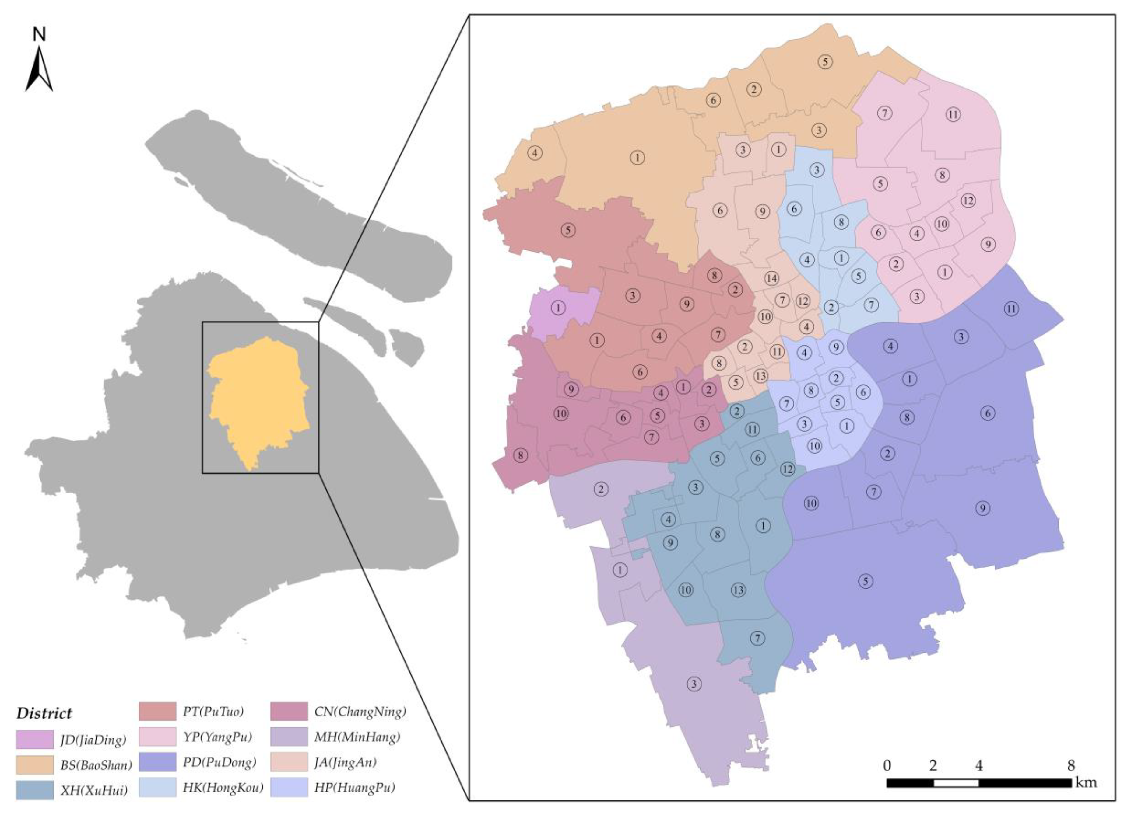
2.1. Study Area
2.2. Bicycle-sharing Data
3. Methodology
3.1. Investigating the Temporal Variation of Bicycle-Sharing Usage
3.2. Urban Vitality Index
3.3. K-Means Clustering
3.4. Examining the Spatial Distribution of the Dynamic Urban Vitality
4. Results
4.1. Temporal Variation of Bicycle-Sharing Usage
4.2. Urban Vitality Clustering
4.3. Spatial Distribution of the Dynamic Urban Vitality
5. Discussion & Conclusions
Author Contributions
Funding
Conflicts of Interest
References
- Ahas, R.; Mark, Ü. Location based services—new challenges for planning and public administration? Futures 2005, 37, 547–561. [Google Scholar] [CrossRef]
- Csáji, B.C.; Browet, A.; Traag, V.A.; Delvenne, J.C.; Huens, E.; Van Dooren, P.; Blondel, V.D. Exploring the mobility of mobile phone users. Phys. A Stat. Mech. Appl. 2013, 392, 1459–1473. [Google Scholar] [CrossRef] [Green Version]
- Do, T.M.T.; Gatica-Perez, D. Where and what: Using smartphones to predict next locations and applications in daily life. Pervasive Mob. Comput. 2014, 12, 79–91. [Google Scholar] [CrossRef] [Green Version]
- Kido, H.; Yanagisawa, Y.; Satoh, T. An anonymous communication technique using dummies for location-based services. In ICPS’05, Proceedings of the International Conference on Pervasive Services, Santorini, Greece, 11–14 July 2005; IEEE: Piscataway, NJ, USA, 2005. [Google Scholar]
- Lu, Y.; Liu, Y.J.C. Pervasive location acquisition technologies: Opportunities and challenges for geospatial studies. Comput. Environ. Urban Syst. 2012, 36, 105–108. [Google Scholar] [CrossRef]
- Hollenstein, L.; Purves, R. Exploring place through user-generated content: Using Flickr tags to describe city cores. J. Spat. Inf. Sci. 2010, 2010, 21–48. [Google Scholar]
- Liu, X.; Gong, L.; Gong, Y.; Liu, Y. Revealing travel patterns and city structure with taxi trip data. J. Transp. Geogr. 2015, 43, 78–90. [Google Scholar] [CrossRef] [Green Version]
- Wan, N.; Lin, G.J.C. Life-space characterization from cellular telephone collected GPS data. Comput. Environ. Urban Syst. 2013, 39, 63–70. [Google Scholar] [CrossRef]
- Wei, M.; Liu, Y.; Sigler, T.; Liu, X.; Corcoran, J. The influence of weather conditions on adult transit ridership in the sub-tropics. Transp. Res. Part A Policy Pract. 2019, 125, 106–118. [Google Scholar] [CrossRef]
- Rekimoto, J.; Miyaki, T.; Ishizawa, T. LifeTag: WiFi-based continuous location logging for life pattern analysis. LoCA 2007, 2007, 35–49. [Google Scholar]
- Kusakabe, T.; Asakura, Y. Behavioural data mining of transit smart card data: A data fusion approach. Transp. Res. Part C Emerg. Technol. 2014, 46, 179–191. [Google Scholar] [CrossRef]
- Zheng, L.; Xia, D.; Zhao, X.; Tan, L.; Li, H.; Chen, L.; Liu, W. Spatial–temporal travel pattern mining using massive taxi trajectory data. Phys. A Stat. Mech. Appl. 2018, 501, 24–41. [Google Scholar] [CrossRef]
- Liu, Y.; Wang, F.; Xiao, Y.; Gao, S. Urban land uses and traffic ‘source-sink areas’: Evidence from GPS-enabled taxi data in Shanghai. Landsc. Urban Plan. 2012, 106, 73–87. [Google Scholar] [CrossRef]
- Ahas, R.; Aasa, A.; Silm, S.; Tiru, M. Daily rhythms of suburban commuters’ movements in the Tallinn metropolitan area: Case study with mobile positioning data. Transp. Res. Part C Emerg. Technol. 2010, 18, 45–54. [Google Scholar] [CrossRef]
- Gong, Y.; Lin, Y.; Duan, Z. Exploring the spatiotemporal structure of dynamic urban space using metro smart card records. Comput. Environ. Urban Syst. 2017, 64, 169–183. [Google Scholar] [CrossRef]
- Ratti, C.; Frenchman, D.; Pulselli, R.M.; Williams, S. Mobile landscapes: Using location data from cell phones for urban analysis. Environ. Plan. B Plan. Des. 2006, 33, 727–748. [Google Scholar] [CrossRef]
- Sevtsuk, A.; Carlo, R. Does urban mobility have a daily routine? Learning from the aggregate data of mobile networks. J. Urban Technol. 2010, 17, 41–60. [Google Scholar] [CrossRef]
- Liu, K.; Gao, S.; Lu, F. Identifying spatial interaction patterns of vehicle movements on urban road networks by topic modelling. Comput. Environ. Urban Syst. 2019, 74, 50–61. [Google Scholar] [CrossRef]
- Zhou, Y.; Fang, Z.; Thill, J.C.; Li, Q.; Li, Y. Functionally critical locations in an urban transportation network: Identification and space–time analysis using taxi trajectories. Comput. Environ. Urban Syst. 2015, 52, 34–47. [Google Scholar] [CrossRef]
- Eren, E.; Uz, V.E. A review on bike-sharing: The factors affecting bike-sharing demand. Sustain. Cities Soc. 2019, 101882. [Google Scholar] [CrossRef]
- Fishman, E.; Washington, S.; Haworth, N. Bike share: A synthesis of the literature. Transp. Rev. 2013, 33, 148–165. [Google Scholar] [CrossRef] [Green Version]
- Nikitas, A. How to save bike-sharing: An evidence-based survival toolkit for policy-makers and mobility providers. Sustainability 2019, 11, 3206. [Google Scholar] [CrossRef] [Green Version]
- Xu, Y.; Chen, D.; Zhang, X.; Tu, W.; Chen, Y.; Shen, Y.; Ratti, C. Unravel the landscape and pulses of cycling activities from a dockless bike-sharing system. Comput. Environ. Urban Syst. 2019, 75, 184–203. [Google Scholar] [CrossRef]
- Caulfield, B.; O’Mahony, M.; Brazil, W.; Weldon, P. Examining usage patterns of a bike-sharing scheme in a medium sized city. Transp. Res. Part A Policy Pract. 2017, 100, 152–161. [Google Scholar] [CrossRef]
- Bakogiannis, E.; Siti, M.; Tsigdinos, S.; Vassi, A.; Nikitas, A. Monitoring the first dockless bike sharing system in Greece: Understanding user perceptions, usage patterns and adoption barriers. Res. Transp. Bus. Manag. 2020, 100432. [Google Scholar] [CrossRef]
- Zhuang, D.; Jin, J.G.; Shen, Y.; Jiang, W. Understanding the bike sharing travel demand and cycle lane network: The case of Shanghai. Int. J. Sustain. Transp. 2019, 1–13. [Google Scholar] [CrossRef]
- Shen, Y.; Zhang, X.; Zhao, J. Understanding the usage of dockless bike sharing in Singapore. Int. J. Sustain. Transp. 2018, 12, 686–700. [Google Scholar] [CrossRef]
- Sung, H.; Lee, S. Residential built environment and walking activity: Empirical evidence of Jane Jacobs’ urban vitality. Transp. Res. Part D Transp. Environ. 2015, 41, 318–329. [Google Scholar] [CrossRef]
- Delclòs-Alió, X.; Gutiérrez, A.; Miralles-Guasch, C. The urban vitality conditions of Jane Jacobs in Barcelona: Residential and smartphone-based tracking measurements of the built environment in a Mediterranean metropolis. Cities 2019, 86, 220–228. [Google Scholar] [CrossRef]
- Lan, F.; Gong, X.; Da, H.; Wen, H. How do population inflow and social infrastructure affect urban vitality? Evidence from 35 large- and medium-sized cities in China. Cities 2019, 102454. [Google Scholar] [CrossRef]
- Anderson, J.; Ruggeri, K.; Steemers, K.; Huppert, F. Lively Social Space, Well-Being Activity, and Urban Design: Findings from a Low-Cost Community-Led Public Space Intervention. Environ. Behav. 2016, 49, 685–716. [Google Scholar] [CrossRef]
- Jacobs, J. The Death and Life of Great American Cities; Random House: New York, NY, USA, 1961. [Google Scholar]
- National Bureau of Statistics of China. China Statistical Yearbook 2019. Available online: http://www.stats.gov.cn/tjsj/ndsj/2019/indexeh.htm (accessed on 6 January 2020).
- Jia, Y.; Ding, D.; Gebel, K.; Chen, L.; Zhang, S.; Ma, Z.; Fu, H. Effects of new dock-less bicycle-sharing programs on cycling: A retrospective study in Shanghai. BMJ Open 2019, 9, e024280. [Google Scholar] [CrossRef] [Green Version]
- Disruptionhub. The 5 Biggest Bike Share Businesses Disrupting Mobility. 2018. Available online: https://disruptionhub.com/bike-share-companies-disrupting-mobility/ (accessed on 26 December 2019).
- Girden, E.R. ANOVA: Repeated Measures; Sage: Newcastle upon Tyne, UK, 1992. [Google Scholar]
- Rosner, B.; Glynn, R.J.; Lee, M.L.T. The Wilcoxon signed rank test for paired comparisons of clustered data. Biometrics 2006, 62, 185–192. [Google Scholar] [CrossRef]
- Guagliardo, M.F. Spatial accessibility of primary care: Concepts, methods and challenges. Int. J. Health Geogr. 2004, 3, 3. [Google Scholar] [CrossRef] [Green Version]
- Handy, S.L.; Niemeier, D.A. Measuring accessibility: An exploration of issues and alternatives. Environ. Plan. A 1997, 29, 1175–1194. [Google Scholar] [CrossRef]
- Pei, T.; Sobolevsky, S.; Ratti, C.; Shaw, S.L.; Li, T.; Zhou, C. A new insight into land use classification based on aggregated mobile phone data. Int. J. Geogr. Inf. Sci. 2014, 28, 1988–2007. [Google Scholar] [CrossRef] [Green Version]
- Zhuo, Y.; Zheng, H.; Wu, C.; Xu, Z.; Li, G.; Yu, Z. Compatibility mix degree index: A novel measure to characterize urban land use mix pattern. Comput. Environ. Urban Syst. 2019, 75, 49–60. [Google Scholar] [CrossRef]
- Hamerly, G.; Elkan, C. Alternatives to the k-means algorithm that find better clusterings. In Proceedings of the Eleventh International Conference on Information and Knowledge Management; ACM: New York, NY, USA, 2002. [Google Scholar]
- Aksoy, S.; Haralick, R.M. Feature normalization and likelihood-based similarity measures for image retrieval. Pattern Recognit. Lett. 2001, 22, 563–582. [Google Scholar] [CrossRef] [Green Version]


| Order_ID | Start_Time | Start_Location | End_Time | End_Location |
|---|---|---|---|---|
| 7971 | 21 August 2016 16:15 | 121.405° E, 31.330° N | 22 August 2016 16:19 | 121.407° E, 31.325° N |
| 8249 | 20 August 2016 16:23 | 121.350° E, 31.262° N | 22 August 2016 16:39 | 121.364° E, 31.260° N |
| 8264 | 20 August 2016 16:24 | 121.386° E, 31.315° N | 22 August 2016 16:30 | 121.377° E, 31.318° N |
| 8320 | 16 August 2016 16:25 | 121.506° E, 31.268° N | 22 August 2016 16:40 | 121.510° E, 31.273° N |
| 8347 | 17 August 2016 16:26 | 121.377° E, 31.217° N | 22 August 2016 16:36 | 121.387° E, 31.214° N |
| 10150 | 18 August 2016 0:00 | 121.528° E, 31.267° N | 18 August 2016 1:56 | 121.577° E, 31.258° N |
| Sum of Squares | Degrees of Freedom | Mean Squares | F Ratio | P-Value | |
|---|---|---|---|---|---|
| Ridership | 243,688 | 6 | 40,615 | 0.697 | 0.652 |
| Residuals | 3.91 × 10⁷ | 672 | 58,233 |
| Monday | Tuesday | Wednesday | Thursday | Friday | Saturday | Sunday | |
|---|---|---|---|---|---|---|---|
| Monday | 1 | 0.223 | 0.174 | 0.291 | 0.104 | 0.029 | 0.006 |
| Tuesday | 1 | 0.141 | 0.089 | 0.534 | 0.016 | 0.015 | |
| Wednesday | 1 | 0.454 | 0.247 | 0.027 | 0.042 | ||
| Thursday | 1 | 0.063 | 0.008 | 0.038 | |||
| Friday | 1 | 0.005 | 0.027 | ||||
| Saturday | 1 | 0.000 | |||||
| Sunday | 1 |
| AM Peak | Midday Off-Peak Hours | PM Peak | Night Hours | |
|---|---|---|---|---|
| Moran’s Index: | 0.258003 | 0.076980 | 0.135361 | 0.174595 |
| Expected Index: | −0.010309 | −0.010309 | −0.010309 | −0.010309 |
| Variance: | 0.001440 | 0.001425 | 0.001331 | 0.001363 |
| z-score: | 7.071193 | 2.312248 | 3.992772 | 5.007999 |
| p-value: | 0.000000 | 0.020764 | 0.000065 | 0.000001 |
© 2020 by the authors. Licensee MDPI, Basel, Switzerland. This article is an open access article distributed under the terms and conditions of the Creative Commons Attribution (CC BY) license (http://creativecommons.org/licenses/by/4.0/).
Share and Cite
Zeng, P.; Wei, M.; Liu, X. Investigating the Spatiotemporal Dynamics of Urban Vitality Using Bicycle-Sharing Data. Sustainability 2020, 12, 1714. https://doi.org/10.3390/su12051714
Zeng P, Wei M, Liu X. Investigating the Spatiotemporal Dynamics of Urban Vitality Using Bicycle-Sharing Data. Sustainability. 2020; 12(5):1714. https://doi.org/10.3390/su12051714
Chicago/Turabian StyleZeng, Peng, Ming Wei, and Xiaoyang Liu. 2020. "Investigating the Spatiotemporal Dynamics of Urban Vitality Using Bicycle-Sharing Data" Sustainability 12, no. 5: 1714. https://doi.org/10.3390/su12051714